RIKEN-MP-58

Hofstadter problem in higher dimensions

Taro Kimura

Institut de Physique Théorique, CEA Saclay, 91191 Gif-sur-Yvette, France
Mathematical Physics Laboratory, RIKEN Nishina Center, Saitama 351-0198, Japan

We investigate some generalizations of the Hofstadter problem to higher dimensions with Abelian and non-Abelian gauge field configurations. We numerically show the hierarchical structure in the energy spectra with several lattice models. It is also pointed out the equivalence between the $\pi$-flux state and the staggered formalism of Dirac fermion.

1 Introduction

The fractal structure of the energy spectrum for the two-dimensional magnetic lattice system, known as Hofstadter’s butterfly [1], is one of the most exotic consequences of the quantum property of the low-dimensionality. Such a fractal nature of the magnetic system can be observed in a simple tight-binding model in the presence of the magnetic field. This Hofstadter problem and its variants have been extensively discussed in various areas of physics and also mathematics. More recently it can be realized even in experimental situations [2, 3].

In this paper we extend the Hofstadter problem, which is originally considered in two dimensions, to higher dimensions with not only Abelian, but also non-Abelian gauge field configuration. So far there are some attempts to generalize it to the three-dimensional magnetic system [4, 5, 6, 7], and also to that in non-Abelian gauge potential [8, 9, 10, 11, 12]. But its generalization to much higher dimensional system has been not yet studied in the literature. Actually, when we analyse topological matters in the lower dimensional system, the four-dimensional point of view can be quite useful: topological insulators/superconductors in two and three dimensions [13, 14] are deeply connected to the four-dimensional QHE [15] through the dimensional reduction procedure [16, 17]. The formalism discussed in this paper can be applied to arbitrary even dimensional lattice system in the presence of the magnetic field. Based on this formalism, we prove the $\pi$-flux state [18, 19], which has a gapless excitation in general, is essentially equivalent to Dirac fermion in arbitrary dimensions. Furthermore, when we apply the non-Abelian gauge field, we can obtain a hierarchical structure in the energy spectrum of the lattice model even in higher dimensions.

This paper is organized as follows. In Sec. 2 we introduce arbitrary even dimensional lattice models with Abelian gauge field background configuration. We discuss the corresponding Schrödinger equation to the magnetic system, and obtain Harper’s equation. We then comment on its connection to the non-commutative torus. We also provide a general proof for the gapless spectrum of the $\pi$-flux state, by referring to its equivalence to the naively discretized lattice Dirac fermion. In Sec. 3 we then consider the Hofstadter problem for the non-Abelian gauge field configuration. In particular the four-dimensional $\mathrm{SU}(2)$ theory is investigated as a fundamental example of the non-Abelian gauge theory. We show some numerical results of the model, and discuss the effect of the inhomogeneity of the background flux. Section 4 is devoted to a summary and discussion.

2 Abelian gauge field models

First generalization of Hofstadter problem is formulated in arbitrary even dimensions in the presence of $\mathrm{U}(1)$ gauge field. Before introducing a lattice model, we now consider the following background $\mathrm{U}(1)$ field configuration for the continuum theory [20],

$$F_{2s-1,2s}=\omega_{s},\quad F_{\mu\nu}=0\quad\mbox{for}\quad\mbox{otherwise},\quad\left(s=1,\cdots,r\right).$$ (2.1)

We then apply the higher dimensional version of Landau gauge to this configuration,

$$A_{2s-1}(x)=-\omega_{s}x_{2s},\qquad A_{2s}(x)=0.$$ (2.2)

Here the field strengths $\omega_{s}$ are quantized,

$$\omega_{s}=\frac{2\pi}{L_{2s-1}L_{2s}}n_{s},\qquad n_{s}\in\mathbb{Z},$$ (2.3)

and thus the topological number is given by

$$Q=\frac{1}{2^{r}\cdot r!}\int d^{2r}x\,\epsilon^{\mu_{1}\cdots\mu_{2r}}\,\mathrm{Tr}\,F_{\mu_{1}\mu_{2}}\cdots F_{\mu_{2r-1},\mu_{2r}}=\prod_{s=1}^{r}n_{s}.$$ (2.4)

This is regarded as the $r$-th Chern number.

To discuss the Hofstadter spectrum, we then realize these configurations on the lattice. The gauge potential (2.2) is implemented by introducing the link variable, which can be regarded as the Wilson line,

$$U_{2s-1}(x)=e^{-i\omega_{s}x_{2s}},\qquad U_{2s}(x)=1.$$ (2.5)

Precisely speaking, we have to assign appropriate boundary conditions even for $U_{2s}(x)$ [20]. In this case the field strength is restricted to the interval $(0,2\pi)$ due to the lattice discretization [21, 22]. Furthermore they are characterized by the following fractions,

$$\frac{p_{s}}{q_{s}}\equiv\frac{n_{s}}{\tilde{L}_{2s-1}\tilde{L}_{2s}},\qquad$$ (2.6)

Here $\tilde{L}_{i}$ is related to the system size as $L_{i}=\tilde{L}a$ where $a$ is the lattice spacing. Note that they satisfy $0<p_{i}/q_{i}<1$. This fraction plays an essential role in the interesting spectrum of the model we discuss below.

2.1 Tight-binding model

The lattice Hamiltonian with this background configuration is defined as

$$\mathcal{H}_{\mathrm{tight}}=\sum_{x,\mu}\left[c_{x+\hat{\mu}}^{\dagger}U_{\mu}(x)c_{x}+c_{x}^{\dagger}U_{\mu}^{\dagger}(x)c_{x+\hat{\mu}}\right].$$ (2.7)

This is just the tight-binding hopping model, which describes the non-relativistic particle with the background magnetic field. Introducing the state $|\psi\rangle=\sum_{x}\psi_{x}c_{x}^{\dagger}|0\rangle$, we obtain the corresponding Schrödinger equation from the Hamiltonian (2.7) written in a second quantized form,

$$\sum_{\mu=1}^{2r}\left[U_{\mu}(x-\hat{\mu})\psi_{x+\hat{\mu}}+U_{\mu}^{\dagger}(x)\psi_{x-\hat{\mu}}\right]=E\psi_{x}.$$ (2.8)

We then solve the equation (2.8) by taking Fourier transformation. Remark the translation symmetry of this model is slightly modified from the usual lattice model due to the background field,

$$x_{2s-1}\sim x_{2s-1}+1,\quad x_{2s}\sim x_{2s}+q_{s}.$$ (2.9)

Thus, writing the coordinate as $x_{2s}=q_{s}y_{s}+z_{s}$, the wavefunction is Fourier transformed as

$$\psi_{x}=\frac{1}{V}\sum_{k_{1},\cdots,k_{2r}}\exp\left[i\sum_{s=1}^{r}\left(k_{2s-1}x_{2s-1}+q_{s}k_{2s}y_{s}\right)\right]\tilde{\psi}_{z_{1},\cdots,z_{r}}(k_{1},\cdots,k_{2r})$$ (2.10)

where $V$ stands for the effective volume of the system, $V=L_{1}\cdots L_{2r}/(q_{1}\cdots q_{r})$. The Schrödinger equation (2.8) is rewritten in this basis as

$$\sum_{s=1}^{r}\left[\tilde{\psi}_{z+\hat{s}}+\tilde{\psi}_{z-\hat{s}}+2\cos\left(k_{2s-1}-\omega_{s}z_{s}\right)\tilde{\psi}_{z}\right]=E\tilde{\psi}_{z}.$$ (2.11)

This is the higher dimensional version of Harper’s equation [23]. While an one-dimensional equation is obtained from the magnetic two-dimensional system, we have a $r$-dimensional equation from the $d=2r$ theory. Furthermore the matrix size of this higher dimensional Harper’s equation is $N_{q}\times N_{q}$ where $N_{q}\equiv q_{1}\cdots q_{r}$. This means that the number of energy bands is just given by $N_{q}$, and there possibly exist $N_{q}-1$ energy gaps. To discuss these energy gaps, one has to investigate a transfer matrix and its spectral curve associated with Harper’s equation (2.11). In this case, however, it is impossible to show these energy bands are totally gapped with the same argument as the two-dimensional situation: we cannot apply a naive transfer matrix method, since there are still $r$ directions in the equation (2.11). Therefore it is difficult to obtain the corresponding Hofstadter’s butterfly by diagonalizing Harper’s equation (2.11): its wings are almost disappearing.

Let me comment on the relationship between the non-commutative space and (2.11). Indeed the higher dimensional tight-binding model, discussed in this section, can be represented in terms of the non-commutative torus. The coordinates of the two-dimensional non-commutative torus $T_{\theta}^{2}$ are given by

$$UV=e^{2\pi i\theta}VU,$$ (2.12)

with $e^{2\pi i\theta}$ being the $q$-th root of unity, $2\pi\theta\equiv\omega=2\pi/q$. They can be written in $q\times q$ matrix forms,

$$U=\left(\begin{array}[]{ccccc}0&1&&&\\ &0&1&&\\ &&\ddots&\ddots&\\ &&&0&1\\ 1&&&&0\\ \end{array}\right),\qquad V=\left(\begin{array}[]{ccccc}1&&&&\\ &e^{i\omega}&&&\\ &&e^{2i\omega}&&\\ &&&\ddots&\\ &&&&e^{(q-1)i\omega}\\ \end{array}\right).$$ (2.13)

Based on this description, we can consider $d=2r$ dimensional non-commutative torus:

$$U_{s}V_{t}=e^{2\pi i\theta_{st}}V_{s}U_{t}\qquad\mbox{for}\quad s,t=1,\cdots,r.$$ (2.14)

In general, $\theta_{st}$ is a real symmetric matrix. In the case of (2.11), it is simply given by a diagonal matrix, $2\pi\theta_{st}=\omega_{s}\delta_{st}$. This means the non-commutativity on the $2r$-dimensional torus is introduced to each two-dimensional subspace, $T_{\theta}^{2r}\to T_{\theta_{1}}^{2}\times\cdots\times T_{\theta_{r}}^{2}$. Then the associated Hamiltonian can be written as

$$\mathcal{H}_{\rm tight}=\sum_{s=1}^{r}\left[U_{s}+U_{s}^{\dagger}+V_{s}+V_{s}^{\dagger}\right].$$ (2.15)

Although, precisely speaking, we have to include a factor corresponding to the plane wave, we now omit these factors for simplicity. This representation means that the non-commutative torus operator plays a role of the translation operator with the external magnetic field even in the higher dimensional case.

2.1.1 $\pi$-flux state

Let us comment on the $\pi$-flux state in higher dimensions. For the $\pi$-flux state [18, 19] all the plaquettes have the same value, $P_{\mu\nu}=-1$, independent of its position $x$, and directions $\mu$, $\nu$ as

$$P_{\mu\nu}(x)=U_{\mu}(x)U_{\nu}(x+\hat{\mu})U_{\mu}^{\dagger}(x+\hat{\nu})U_{\nu}^{\dagger}(x)=-1.$$ (2.16)

Such a configuration is realized by the following $\mathbb{Z}_{2}\subset\mathrm{U}(1)$ link variables,

$$U_{\mu}(x)=\eta_{\mu}\equiv(-1)^{x_{1}+\cdots+x_{\mu-1}}.$$ (2.17)

Then the tight-binding Hamiltonian in the second quantized form with this gauge configuration yields

$$\mathcal{H}_{\rm tight}=\sum_{x}\sum_{\mu=1}^{d}\eta_{\mu}c_{x}^{\dagger}\left(c_{x+\hat{\mu}}+c_{x-\hat{\mu}}\right).$$ (2.18)

We now consider the free field theory for simplicity. This is almost the same as the staggered Dirac operator [26, 27, 28]

$$\mathcal{S}_{\rm staggered}=\sum_{x}\sum_{\mu=1}^{d}\frac{1}{2}\eta_{\mu}\bar{\chi}_{x}\left(\chi_{x+\hat{\mu}}-\chi_{x-\hat{\mu}}\right).$$ (2.19)

Actually, by applying the transformation $c_{x}\to i^{x_{1}+\cdots+x_{d}}c_{x}$, the Hamiltonian (2.18) is rewritten as

$$\mathcal{H}_{\rm tight}=\sum_{x}\sum_{\mu=1}^{d}i\,\eta_{\mu}c_{x}^{\dagger}\left(c_{x+\hat{\mu}}-c_{x-\hat{\mu}}\right).$$ (2.20)

This is just the staggered fermion action (2.19), up to a constant factor. Note that the staggered Dirac operator is anti-Hermitian while the tight-binding Hamiltonian is Hermitian.

There is no spinor structure in this formulation, but this staggered fermion is directly obtained from the naive Dirac fermion through the spin-diagonalization. See Appendix A for details. The sign factor $\eta_{\mu}=(-1)^{x_{1}+\cdots+x_{\mu-1}}$ is a remnant of the gamma matrix. The staggered fermion enjoys an exact $\mathrm{U}(1)$ chiral symmetry, which is generated by $\epsilon_{x}=(-1)^{x_{1}+\cdots+x_{d}}$. This symmetry ensures its gapless excitation. Therefore the $\pi$-flux state is also generically gapless.

2.2 Dirac fermion models

We then attempt to extend the Hofsdater’s problem to the relativistic system. Similar approaches have been seen in the context of graphene [29, 30, 31, 32].

The generic form of the Dirac fermion action is written as

$$\mathcal{S}_{\mathrm{Dirac}}=\sum_{x,\mu}\left[\bar{\psi}_{x+\hat{\mu}}U_{\mu}(x)P_{\mu}^{+}\psi_{x}-\bar{\psi}_{x}U^{\dagger}_{\mu}(x)P_{\mu}^{-}\psi_{x+\hat{\mu}}\right]\equiv\sum_{x,y}\bar{\psi}_{x}D_{x,y}\psi_{y}.$$ (2.21)

Here $P_{\mu}^{\pm}$ stands for the spinor matrix, corresponding to a type of the lattice fermion. The simplest one is given by

$$P_{\mu}^{\pm}=\frac{1}{2}\gamma_{\mu}.$$ (2.22)

This is just the naive lattice discretization of the relativistic fermion [34]. We have other choices for the spinor matrix:

• Wilson fermion [34]

  $$P_{\mu}^{\pm}=\frac{1}{2}(\gamma_{\mu}\pm r\mathbbm{1})$$ (2.23)

• Karsten–Wilczek fermion [36, 37]

  $$P_{\mu}^{\pm}=\frac{1}{2}\gamma_{\mu}\quad(\mu=d),\qquad P_{\mu}^{\pm}=\frac{1}{2}(\gamma_{\mu}\pm ir\gamma_{d})\quad(\mbox{otherwise})$$ (2.24)

• Boriçi–Creutz fermion [38, 39]

  $$P_{\mu}^{\pm}=\frac{1}{2}\left((1\pm ir)\gamma_{\mu}\mp ir\Gamma\right),\qquad\Gamma=\frac{1}{2}\sum_{\mu=1}^{d}\gamma_{\mu}$$ (2.25)

All these fermions include a free parameter $r$. We often consider the case of $r=1$ for simplicity. Note that another lattice fermion, which is called the staggered fermion [26, 27, 28], is essentially equivalent to the naive fermion, and also the $\pi$-flux state as discussed in section 2.1. The naive and staggered fermions are transformed to each other by the spin-diagonalization. Thus in this paper we do not deal with the staggered fermion explicitly.

The Dirac equation, which corresponds to the Schrödinger equation (2.8), is given by

$$\sum_{\mu=1}^{d}\left[U_{\mu}(x)P^{+}_{\mu}\psi_{x+\hat{\mu}}-U_{\mu}^{\dagger}(x-\hat{\mu})P^{-}_{\mu}\psi_{x-\hat{\mu}}\right]=\lambda\psi_{x}.$$ (2.26)

When we write this equation (2.26) as $D\psi=\lambda\psi$, although this Dirac operator $D$ becomes non-Hermitian in general, one can define an alternative Hermitian operator, $H=\gamma_{d+1}D$. In the following we consider the spectrum of this Hermitian operator as $H\psi=E\psi$, instead of the original Dirac equation (2.26).

We can also obtain the corresponding Harper’s equation by taking Fourier transformation. In this case, Harper’s equation is slightly modified from (2.11) as

$$\sum_{s=1}^{d/2}\gamma_{d+1}\Big{[}P^{+}_{2s}\tilde{\psi}_{z+\hat{s}}-P^{-}_{2s}\tilde{\psi}_{z-\hat{s}}$$

$$+\Big{(}i\sin\left(k_{2s-1}-\omega_{s}z_{s}\right)\left(P_{2s-1}^{+}+P_{2s-1}^{-}\right)+\cos\left(k_{2s-1}-\omega_{s}z_{s}\right)\left(P_{2s-1}^{+}-P_{2s-1}^{-}\right)\Big{)}\tilde{\psi}_{z}\Big{]}=E\tilde{\psi}_{z}.$$

(2.27)

Here we have $2N_{q}$ energy bands due to the $\gamma$-matrix structure: they appear in a pair for the relativistic theory. In this case, it is again difficult to obtain a fully gapped spectrum since this reduced equation is not one-dimensional, but $d/2$-dimensional.

3 Non-Abelian gauge field models

We consider another generalization of the Hofstadter problem in higher dimensions by applying a non-Abelian gauge field as a background configuration. In this paper we concentrate on the four-dimensional model with $\mathrm{SU}(2)$ gauge field. A further generalization to higher dimensional, and higher rank systems seems to be straightforward.

3.1 Background configuration

We now introduce the following $\mathrm{SU}(2)$ background configuration as a simple generalization of the $\mathrm{U}(1)$ background (2.2),

$$A_{0}=0,\qquad A_{j}=-\omega_{j}x_{0}\sigma_{j}\quad\mbox{for}\quad j=1,2,3,$$ (3.1)

with $\sigma_{j}$ being the Pauli matrix. Here we define filling fractions

$$\omega_{j}=\frac{2\pi}{L^{2}}n_{j}\equiv 2\pi\frac{p_{j}}{q_{j}}.$$ (3.2)

From this configuration we compute a field strength,

$$F_{0j}=-\omega_{j}\sigma_{j},\qquad F_{jk}=-\omega_{j}\omega_{k}x_{0}^{2}\epsilon_{ijk}\sigma^{i}.$$ (3.3)

The total background flux is given by

$$\frac{1}{16\pi^{2}}\int_{L^{4}}d^{4}x\,\epsilon^{\mu\nu\rho\sigma}\,\mathrm{Tr}\,F_{\mu\nu}F_{\rho\sigma}=\frac{6\pi^{2}}{L^{6}}N\int_{L^{4}}d^{4}x\,x_{0}^{2}=2\pi N.$$ (3.4)

Here this integral is taken over the four-dimensional hypercubic lattice of the size $L^{4}$, and we define the flux number $N=n_{1}n_{2}n_{3}$.

Thus the link variables associated with (3.1) are given as follows,

$$U_{0}(x)=\mathbbm{1},\qquad U_{j}(x)=e^{-i\omega_{j}x_{0}\sigma_{j}}=\mathbbm{1}\cos\omega_{j}x_{0}-i\sigma_{j}\sin\omega_{j}x_{0}.$$ (3.5)

In this case, the translation symmetry of the lattice system yields

$$x_{0}\sim x_{0}+q_{\rm LCM},\qquad x_{j}\sim x_{j}+1,$$ (3.6)

where $q_{\rm LCM}$ is the least common multiple of $q_{1},q_{2}$ and $q_{3}$. This means that the unit cell of this system is also extended in only one dimension as well as the two-dimensional case with $\mathrm{U}(1)$ magnetic field.

3.2 Lattice fermion models

Let us first study the tight-binding model with the non-Abelian gauge field configuration. With a Fourier basis for $x_{0}=q_{\rm LCM}X_{0}+\bar{x}_{0}$, the Hamiltonian (2.7) gives rise to the corresponding Harper’s equation (2.11),

$$\tilde{\psi}_{\bar{x}_{0}+1}+\tilde{\psi}_{\bar{x}_{0}-1}+2\sum_{j=1}^{3}\Big{(}\cos k_{j}\cos\omega_{j}\bar{x}_{0}+\sigma_{j}\sin k_{j}\sin\omega_{j}\bar{x}_{0}\Big{)}\tilde{\psi}_{\bar{x}_{0}}=E\tilde{\psi}_{\bar{x}_{0}}.$$ (3.7)

This is just an effective one-dimensional model as the standard two-dimensional Hofstadter problem. The original four-dimensional model is reduced to this due to $\mathrm{SU}(2)\cong S^{3}$ gauge symmetry. On the other hand, in this case it is also difficult to show its spectrum is totally gapped as the case of the $\mathrm{U}(1)$ background in higher dimensions. Therefore we now study its density of states instead of the original energy spectrum.

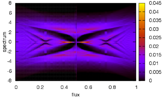
Figure 1: Density of states for Harper’s equation (3.7) of the flux $\omega_{j=1,2,3}=\omega_{0}\equiv 2\pi p/q$ with $q=100$, $p=0,1,2,\cdots 99$.

Fig. 1 shows the density of states for Harper’s equation (3.7) against $\omega_{0}$, with homogeneous configuration $\omega_{j}=\omega_{0}$ for $j=1,2,3$. Although its spectrum is not totally gapped, one can observe a hierarchical structure of the spectrum, which seems fractal at least based on this numerical computation. In order to numerically determine the corresponding fractal dimension, it is necessary to perform the calculation with a larger size system. At the even fraction flux, e.g. $\omega_{0}/(2\pi)=1/2,1/4,\cdots$, we find a dip in the spectrum. Similar structure is discussed in the ordinary two-dimensional Hofstadter problem at the gapless point of the filling fraction.

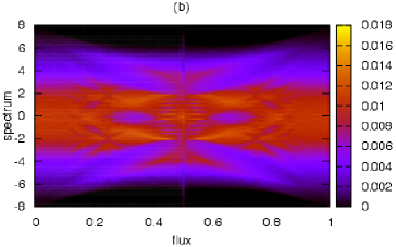
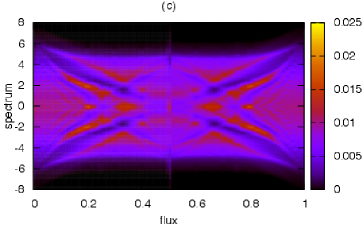
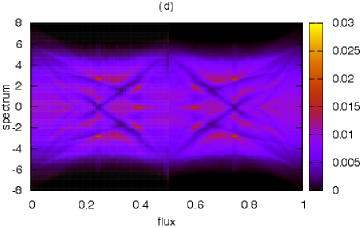
Figure 2: Density of states for Harper’s equation (3.7) with the inhomogeneous flux for $\vec{\omega}=\omega_{0}\vec{n}$: (a) $\vec{n}=(1,0,0)$, (b) $(1,1,0)$, (c) $(2,1,1)$, and (d) $(2,2,1)$.

In Fig. 2 we show the spectrum in the inhomogeneous flux with fixing ratios of $\omega_{j=1,2,3}$. When flux in some directions is turned off, e.g. $\vec{\omega}=\omega_{0}(1,0,0)$ and $\omega_{0}(1,1,0)$, the characteristic structure of Hofstadter’s butterfly cannot be observed in the spectrum: gap is completely closed. In the cases of $\vec{\omega}=\omega_{0}(2,1,1)$ and $\omega_{0}(2,2,1)$, there are some gaps in the spectrum and the hierarchical structure. We also find a dip at the gapless point, $\omega_{0}=\pi$.

Let us now comment on the relation to the non-commutative space. We introduce the following non-commutative torus,

$$UV_{j}=e^{i\omega_{j}\sigma_{j}}V_{j}U\qquad\mbox{for}\quad j=1,2,3.$$ (3.8)

Here $U$ is defined as well as (2.13), while $V_{j=1,2,3}$ are slightly modified as

$$V_{j}=\mathrm{diag}\left(1,\,e^{i\omega_{j}\sigma_{j}},\,\cdots,\,e^{(q_{\rm LCM}-1)i\omega_{j}\sigma_{j}}\right).$$ (3.9)

In this case the non-commutative parameter is matrix valued. Thus, the commutation relations between $V_{j=1,2,3}$ cannot be written in a simple way.

As discussed in Sec. 2, the tight-binding Hamiltonian with the external field, corresponding to Harper’s equation (3.7), can be associated with the non-commutative torus. The naive form of the Hamiltonian without momentum dependence is given by

$$U+U^{\dagger}+\sum_{j=1}^{3}\left[V_{j}+V_{j}^{\dagger}\right].$$ (3.10)

However, since the second part is represented as

$$V_{j}+V_{j}^{\dagger}=\mathrm{diag}\left(2,\,2\cos\omega_{j},\,\cdots,\,2\cos(q_{\rm LCM}-1)\omega_{j}\right)\times\mathbbm{1},$$ (3.11)

we cannot involve a matrix structure in this way. Actually the $\mathrm{SU}(2)$ nature of the external field is coming through the momentum dependence in (3.7).

We then investigate the Dirac fermion models as discussed in section 2.2. Applying the background configuration (3.5), the corresponding Dirac equation is given by

$$\gamma_{5}\Big{[}P_{0}^{+}\tilde{\psi}_{\bar{x}_{0}+1}-P_{0}^{-}\tilde{\psi}_{\bar{x}_{0}-1}$$

$$+\sum_{j=1}^{3}\Big{(}\left(\cos k_{j}\cos\omega_{j}\bar{x}_{0}+\sigma_{j}\sin k_{j}\sin\omega_{j}\bar{x}_{0}\right)\left(P_{j}^{+}-P_{j}^{-}\right)$$

$$\hskip 25.00003pt+\left(\sin k_{j}\cos\omega_{j}\bar{x}_{0}-\sigma_{j}\cos k_{j}\sin\omega_{j}\bar{x}_{0}\right)\left(P_{j}^{+}+P_{j}^{-}\right)\Big{)}\tilde{\psi}_{\bar{x}_{0}}\Big{]}=E\tilde{\psi}_{\bar{x}_{0}}.$$ (3.12)

Here we again show the Hermitian version of the Dirac equation by multiplying the matrix $\gamma_{5}$. When we write this Dirac operator in a matrix form, its matrix size is $8q_{\rm LCM}=2$ (color) $\times$ 4 (spinor) $\times$ $q_{\rm LCM}$ (flux). Here color corresponds to the rank of the gauge flux of $\mathrm{SU}(2)$. On the other hand, the number of eigenvalues is given by $4q_{\rm LCM}$, since each spectrum is doubly degenerated due to the spinor structure.

4 Summary and discussions

In this paper we have explored some extensions of the Hofstadter problem in higher dimensions. First example is formulated with Abelian gauge configuration in $d=2r$, giving rise to non-zero topological number. We have shown that half of the gauge potential can be trivial by applying the Landau gauge, thus the corresponding Harper’s equation is essentially written as $r$-dimensional lattice model.

We have also pointed out that the $\pi$-flux state is equivalent to the staggered formalism of the relativistic lattice fermion. The latter is directly related to the naive Dirac fermion through the spin diagonalization. This means the $\pi$-flux state involves the chiral symmetry, and thus it yields massless excitation in any dimensions.

We have then investigated $\mathrm{SU}(2)$ non-Abelian gauge field configuration in four dimensions. We have considered the configuration with one specific direction in four dimensions. In this case hopping terms for the other three directions are reduced due to $\mathrm{SU}(2)\cong S^{3}$ symmetry of the gauge field. Thus we have obtained the one-dimensional Harper’s equation by utilizing the Fourier basis. We have calculated its spectrum numerically, and its hierarchical structure is actually observed.

Let us now comment on possibilities of future works along this direction. The two-dimensional Hofstadter problem is essentially related to the quantum group [40, 41, 42, 29]: Harper’s equation is directly regarded as the Baxter’s equation for the one-dimensional $U_{q}(\mathfrak{sl}_{2})$ model. Thus it is interesting to explore the corresponding quantum group structure to the generalized Hofstadter problems discussed in this paper. In particular, the non-Abelian version of Harper’s equation includes the matrix-valued coefficient. This corresponds to $q$-parameter in the two-dimensional case, thus it is natural to investigate a kind of quantum group with matrix-valued $q$-parameter.

Next is the lattice study with various kinds of lattice fermions, i.e. Wilson [34], staggered [26, 27, 28], staggered-Wilson [43, 44, 45, 46, 47], minimal-doubling [36, 37, 38, 39, 48, 49, 50], domain-wall [51, 52, 53] and overlap fermions [54]. They were originally introduced to tackle the difficulty of the chiral fermion on the lattice, but these formalisms themselves are interesting as statistical lattice models: some of them are actually investigated in the context of condensed-matter physics, for example, graphene, $\pi$-flux state, topological insulator/superconductor and so on. Thus we hope the Hofstadter problem formulated with these lattice fermions are relevant to realistic condensed-matter physics.

It is also definitely interesting to consider implications of the result obtained in this paper for realistic situations. An important difference between the non-Abelian gauge field and the $\mathrm{U}(1)$ magnetic field is whether it breaks the time-reversal symmetry of the system: the $\mathrm{SU}(2)$ gauge potential can be applied without breaking the time-reversal symmetry. It implies that, as a consequence of the dimensional reduction of the model discussed in this paper, one can possibly realize the non-Abelian Hofstadter system, for example, in topological insulators whose time-reversal symmetry is not broken. In addition, since there are already experimental techniques to realize the non-Abelian gauge potential and the ordinary Hofstadter system based on the $\mathrm{U}(1)$ field, respectively, one can expect that experimental realization of the non-Abelian Hofstadter system might be possible especially in the cold atomic system.

Acknowledgments

The author would like to thank M. Creutz, Y. Hidaka and T. Misumi for useful discussions and comments. The author is grateful to H. Iida for collaboration at the early stage of this work. The author is supported by Grant-in-Aid for JSPS Fellows (No. 23-593).

Appendix A Spin diagonalization

We now show that there is an alternative expression of the $d$-dimensional naive Dirac fermion without spinor matrix structure. It is given by diagonalizing the corresponding $\gamma$ matrices.

Let us start with the naive Dirac fermion on the lattice,

$$\mathcal{S}=\sum_{x,\mu}\left[\frac{1}{2}\bar{\psi}_{x}\gamma_{\mu}\left(\psi_{x+\hat{\mu}}-\psi_{x-\hat{\mu}}\right)+m\bar{\psi}_{x}\psi_{x}\right].$$ (A.1)

Then, introducing the field $\chi_{x}$ defined as

$$\psi_{x}=\gamma_{d}^{x_{d}}\cdots\gamma_{2}^{x_{2}}\gamma_{1}^{x_{1}}\chi_{x},\qquad\bar{\psi}_{x}=\bar{\chi}_{x}\gamma_{1}^{x_{1}}\gamma_{2}^{x_{2}}\cdots\gamma_{d}^{x_{d}},$$ (A.2)

we can represent the naive lattice fermion (A.1) in the following form,

$$\mathcal{S}=\sum_{x,\mu}\left[\frac{1}{2}\eta_{\mu}(x)\bar{\chi}_{x}\left(\chi_{x+\hat{\mu}}-\chi_{x-\hat{\mu}}\right)+m\bar{\chi}_{x}\chi_{x}\right]\qquad\mbox{with}\qquad\eta_{\mu}(x)=(-1)^{\sum_{\nu<\mu}x_{\nu}}.$$ (A.3)

Remark there is no spinor structure in this expression. In other words, the spinor matrix is diagonalized in this basis. This means the naive Dirac fermion can be rewritten in terms of one-component fermionic field. This is just the staggered formalism of the relativistic fermion [27, 28].

References

- [1] D. R. Hofstadter, “Energy levels and wave functions of Bloch electrons in rational and irrational magnetic fields,” Phys. Rev. B14 (1976) 2239–2249.
- [2] M. Aidelsburger, M. Atala, M. Lohse, J. T. Barreiro, B. Paredes, and I. Bloch, “Realization of the Hofstadter Hamiltonian with ultracold atoms in optical lattices,” Phys. Rev. Lett. 111 (2013) 185301, arXiv:1308.0321 [cond-mat.quant-gas].
- [3] H. Miyake, G. A. Siviloglou, C. J. Kennedy, W. Cody Burton, and W. Ketterle, “Realizing the Harper Hamiltonian with Laser-Assisted Tunneling in Optical Lattices,” Phys. Rev. Lett. 111 (2013) 185302, arXiv:1308.1431 [cond-mat.quant-gas].
- [4] Y. Hasegawa, “Generalized Flux States on 3-Dimensional Lattice,” J. Phys. Soc. Jpn. 59 (1990) 4384–4393.
- [5] Z. Kunszt and A. Zee, “Electron hopping in three-dimensional flux states,” Phys. Rev. B44 (1991) 6842–6848.
- [6] M. Kohmoto, B. I. Halperin, and Y.-S. Wu, “Diophantine equation for the three-dimensional quantum Hall effect,” Phys. Rev. B45 (1992) 13488–13493.
- [7] M. Koshino, H. Aoki, K. Kuroki, S. Kagoshima, and T. Osada, “Hofstadter Butterfly and Integer Quantum Hall Effect in Three Dimensions,” Phys. Rev. Lett. 86 (2001) 1062–1065, arXiv:cond-mat/0006393 [cond-mat.mes-hall].
- [8] N. Goldman and P. Gaspard, “Quantum Hall-like effect for cold atoms in non-Abelian gauge potentials,” Europhys. Lett. 78 (2007) 60001, arXiv:cond-mat/0609472 [cond-mat.mes-hall].
- [9] N. Goldman, “Spatial patterns in optical lattices submitted to gauge potentials,” Europhys. Lett. 80 (2007) 20001, arXiv:0707.3727 [cond-mat.mes-hall].
- [10] N. Goldman, A. Kubasiak, P. Gaspard, and M. Lewenstein, “Ultracold atomic gases in non-Abelian gauge potentials: The case of constant Wilson loop,” Phys. Rev. A79 (2009) 023624, arXiv:0902.3228 [cond-mat.mes-hall].
- [11] N. Goldman, A. Kubasiak, A. Bermudez, P. Gaspard, M. Lewenstein, and M. A. Martin-Delgado, “Non-Abelian optical lattices: Anomalous quantum Hall effect and Dirac Fermions,” Phys. Rev. Lett. 103 (2009) 035301, arXiv:0903.2464 [cond-mat.mes-hall].
- [12] D. Cocks, P. P. Orth, S. Rachel, M. Buchhold, K. Le Hur, and W. Hofstetter, “Time-Reversal-Invariant Hofstadter–Hubbard Model with Ultracold Fermions,” Phy. Rev. Lett. 109 (2012) 205303, arXiv:1204.4171 [cond-mat.quant-gas].
- [13] M. Z. Hasan and C. L. Kane, “Topological insulators,” Rev. Mod. Phys. 82 (2010) 3045, arXiv:1002.3895 [cond-mat.mes-hall].
- [14] M. Z. Hasan and J. E. Moore, “Three-Dimensional Topological Insulators,” Ann. Rev. Cond. Mat. Phys. 2 (2011) 55–78, arXiv:1011.5462 [cond-mat.str-el].
- [15] S.-C. Zhang and J. Hu, “A Four Dimensional Generalization of the Quantum Hall Effect,” Science 294 (2001) 823, arXiv:cond-mat/0110572.
- [16] X.-L. Qi, T. Hughes, and S.-C. Zhang, “Topological Field Theory of Time-Reversal Invariant Insulators,” Phys. Rev. B78 (2008) 195424, arXiv:0802.3537 [cond-mat.mes-hall].
- [17] S. Ryu, A. P. Schnyder, A. Furusaki, and A. W. W. Ludwig, “Topological insulators and superconductors: tenfold way and dimensional hierarchy,” New J. Phys. 12 (2010) 065010, arXiv:0912.2157 [cond-mat.mes-hall].
- [18] I. Affleck and J. B. Marston, “Large- limit of the Heisenberg-Hubbard model: Implications for high- superconductors,” Phys. Rev. B37 (1988) 3774–3777.
- [19] J. B. Marston and I. Affleck, “Large- limit of the Hubbard-Heisenberg model,” Phys. Rev. B39 (1989) 11538–11558.
- [20] J. Smit and J. C. Vink, “Remnants of the Index Theorem on the Lattice,” Nucl. Phys. B286 (1987) 485–508.
- [21] C. Panagiotakopoulos, “Topology of 2D lattice gauge fields,” Nucl.Phys. B251 (1985) 61–76.
- [22] A. Phillips, “Characteristic numbers of -valued lattice gauge fields,” Annals Phys. 161 (1985) 399–422.
- [23] P. G. Harper, “Single Band Motion of Conduction Electrons in a Uniform Magnetic Field,” Proc. Phys. Soc. A68 (1955) 874.
- [24] G. Grignani and G. W. Semenoff, Field Theories for Low-Dimensional Condensed Matter Systems, ch. Introduction to Some Common Topics in Gauge Theory and Spin Systems, pp. 171–233. Springer, 2000.
- [25] M. Creutz, “Emergent spin,” Annals Phys. 342 (2014) 21–30, arXiv:1308.3672 [hep-lat].
- [26] J. B. Kogut and L. Susskind, “Hamiltonian Formulation of Wilson’s Lattice Gauge Theories,” Phys. Rev. D11 (1975) 395.
- [27] L. Susskind, “Lattice Fermions,” Phys. Rev. D16 (1977) 3031.
- [28] H. S. Sharatchandra, H. J. Thun, and P. Weisz, “Susskind Fermions on a Euclidean Lattice,” Nucl. Phys. B192 (1981) 205.
- [29] M. Kohmoto and A. Sedrakyan, “Hofstadter problem on the honeycomb and triangular lattices: Bethe ansatz solution,” Phys. Rev. B73 (2006) 235118, arXiv:cond-mat/0603285 [cond-mat.mes-hall].
- [30] Y. Hasegawa and M. Kohmoto, “Quantum Hall effect and the topological number in graphene,” Phys. Rev. B74 (2006) 155415, arXiv:cond-mat/0603345 [cond-mat.dis-nn].
- [31] N. Nemec and G. Cuniberti, “Hofstadter butterflies of carbon nanotubes: Pseudofractality of the magnetoelectronic spectrum,” Phys. Rev. B74 (2006) 165411, arXiv:cond-mat/0607096 [cond-mat.mes-hall].
- [32] N. Nemec and G. Cuniberti, “Hofstadter butterflies of bilayer graphene,” Phys. Rev. B75 (2007) 201404, arXiv:cond-mat/0612369 [cond-mat.mes-hall].
- [33] T. Kimura, S. Komatsu, T. Misumi, T. Noumi, S. Torii, and S. Aoki, “Revisiting symmetries of lattice fermions via spin-flavor representation,” JHEP 01 (2012) 048, arXiv:1111.0402 [hep-lat].
- [34] K. G. Wilson, “Confinement of quarks,” Phys. Rev. D10 (1974) 2445.
- [35] M. Creutz, “Confinement, chiral symmetry, and the lattice,” Acta Phys. Slov. 61 (2011) 1–127, arXiv:1103.3304 [hep-lat].
- [36] L. H. Karsten, “Lattice fermions in euclidean space-time,” Phys. Lett. B104 (1981) 315.
- [37] F. Wilczek, “Lattice Fermions,” Phys. Rev. Lett. 59 (1987) 2397.
- [38] M. Creutz, “Four-dimensional graphene and chiral fermions,” JHEP 0804 (2008) 017, arXiv:0712.1201 [hep-lat].
- [39] A. Boriçi, “Creutz fermions on an orthogonal lattice,” Phys. Rev. D78 (2008) 074504, arXiv:0712.4401 [hep-lat].
- [40] P. B. Wiegmann and A. V. Zabrodin, “Bethe-ansatz for the Bloch electron in magnetic field,” Phys. Rev. Lett. 72 (1994) 1890.
- [41] P. B. Wiegmann and A. V. Zabrodin, “Quantum Group and Magnetic Translations: Bethe Ansatz Solution for the Harper’s Equation,” Mod. Phys. Lett. B8 (1994) 311–318, arXiv:cond-mat/9310017 [cond-mat].
- [42] Y. Hatsugai, M. Kohmoto, and Y.-S. Wu, “Quantum group, Bethe ansatz equations, and Bloch wave functions in magnetic fields,” Phys. Rev. B53 (1996) 9697–9712, arXiv:cond-mat/9509062.
- [43] D. H. Adams, “Theoretical foundation for the Index Theorem on the lattice with staggered fermions,” Phys. Rev. Lett. 104 (2010) 141602, arXiv:0912.2850 [hep-lat].
- [44] D. H. Adams, “Pairs of chiral quarks on the lattice from staggered fermions,” Phys. Lett. B699 (2011) 394–397, arXiv:1008.2833 [hep-lat].
- [45] C. Hoelbling, “Single flavor staggered fermions,” Phys. Lett. B696 (2011) 422–425, arXiv:1009.5362 [hep-lat].
- [46] M. Creutz, T. Kimura, and T. Misumi, “Aoki Phases in the Lattice Gross-Neveu Model with Flavored Mass terms,” Phys. Rev. D83 (2011) 094506, arXiv:1101.4239 [hep-lat].
- [47] T. Misumi, T. Z. Nakano, T. Kimura, and A. Ohnishi, “Strong-coupling Analysis of Parity Phase Structure in Staggered-Wilson Fermions,” Phy. Rev. D86 (2012) 034501, arXiv:1205.6545 [hep-lat].
- [48] T. Kimura and T. Misumi, “Characters of Lattice Fermions Based on the Hyperdiamond Lattice,” Prog. Theor. Phys. 124 (2010) 415–432, arXiv:0907.1371 [hep-lat].
- [49] T. Kimura and T. Misumi, “Lattice Fermions Based on Higher-Dimensional Hyperdiamond Lattices,” Prog. Theor. Phys. 123 (2010) 63–78, arXiv:0907.3774 [hep-lat].
- [50] M. Creutz and T. Misumi, “Classification of Minimally Doubled Fermions,” Phys. Rev. D82 (2010) 074502, arXiv:1007.3328 [hep-lat].
- [51] D. B. Kaplan, “A Method for simulating chiral fermions on the lattice,” Phys. Lett. B288 (1992) 342, arXiv:hep-lat/9206013.
- [52] Y. Shamir, “Chiral fermions from lattice boundaries,” Nucl. Phys. B406 (1993) 90–106, arXiv:hep-lat/9303005.
- [53] V. Furman and Y. Shamir, “Axial symmetries in lattice QCD with Kaplan fermions,” Nucl. Phys. B439 (1995) 54, arXiv:hep-lat/9405004.
- [54] H. Neuberger, “More about exactly massless quarks on the lattice,” Phys. Lett. B427 (1998) 353, arXiv:hep-lat/9801031.