Adiabatic piston in a temperature gradient

Abstract

The steady states of two gases of hard spheres or disks separated by an adiabatic piston in presence of a temperature gradient are discussed. The temperature field is generated by two thermal walls at different temperatures, each of them in contact with one of the gases. The presence of the piston strongly affects the hydrodynamic fields, inducing a jump in its vicinity. A simple kinetic theory model is formulated. Its predictions are shown to be in good agreement with molecular dynamics simulation results. The applicability of the minimum entropy production principle is analyzed, and it is found that it only provides an accurate description of the system in the limit of a small temperature gradient.

Keywords: Non-equilibrium and irreversible thermodynamics, Kinetic theory, Fluctuation phenomena, random processes, noise, and Brownian motion

The adiabatic piston consists of a container filled with a gas that is divided into two compartments by a freely moving adiabatic piston [1]. Usually, the system is isolated and initially prepared with the two gases in both compartments at different independent states. Then, the relaxation to equilibrium is studied. It is observed that the system first converges towards a state of mechanical equilibrium with both gases having the same pressure. Then, the pressure fluctuations that are asymmetrical because the temperatures of the gases are different, drive the system very slowly to thermal equilibrium [2, 3]. Of course, the situation is much more complex and less understood when the system can not relax to equilibrium due to some imposed external conditions. Very recently, several configurations consisting of granular gases separated by an adiabatic piston have been considered [4, 5, 6]. Granular gases are inherent non-equilibrium systems, since no equilibrium state is possible for them and, for this reason, they have been intensively used to investigate many fundamental issues in the context of non-equilibrium statistical mechanics [7, 8]. Nevertheless, it must be realized that the irreversibility in granular gases has an internal origin, and it is not related, in principle, to some imposed boundary or initial conditions, as it is the case in molecular systems. Actually, as a consequence of the above, gradients and inelasticity are related in steady granular gases and this leads to a quite peculiar rheological behavior.

The aim of this paper is to study the steady state of two molecular gases separated by an adiabatic piston, when each of the gases is in contact with a thermal wall at different temperature. Attention will be restricted to the final state of the system, whithout studying the way in which it is reached. The questions addressed are related with the modification of the hydrodynamic steady profiles because of the presence of the piston and the steady position of the latter.

The system considered is a rectangular ($d=2$) or cylindrical ($d=3$) container of length $L_{x}$. It is divided into two compartments by a movable adiabatic piston of mass $M$, constrained to remain perpendicular to the axis of the system, taken as $x$-axis. By adiabatic it is meant, as usual, that the piston has no internal degrees of freedom and, therefore, it can not transmit energy when it is at rest. A sketch of the system is given in Fig. 1. In each of the two compartment there are $N$ elastic hard disks ($d=2$) or spheres ($d=3$) of mass $m$ and diameter $\sigma$. Collisions between particles and the piston as well as collisions of the particles with the lateral walls of the container are also elastic. Moreover, the motion of the piston occurs without friction with the lateral walls.

Figure 1: Sketch of the system considered in this work. The left and right walls are thermal with temperatures $T_{10}$ and $T_{20}$, respectively.

The walls of the container located at $x=0$ and $x=L_{x}$ and perpendicular to the $x$-axis are thermal walls with temperatures $T_{10}$ and $T_{20}$, respectively. At the microscopic level of description, a thermal wall is modeled by assuming that whenever a particle collides with it, a new velocity is assigned to the particle drawn from a Maxwellian distribution with a second moment defined by the temperature of the wall [9, 10]. More specifically, the velocity distribution of the particles leaving a thermal wall with temperature $T_{i0}$, $i=1,2$, is given by

$$P({\bm{v}})=\theta\left[(-1)^{i-1}v_{x}\right]\left(2\pi\right)^{-\frac{d-1}{2}}\left(\frac{m}{k_{B}T_{i0}}\right)^{\frac{d+1}{2}}v_{x}\exp\left(-\frac{mv^{2}}{2k_{B}T_{i0}}\right),$$ (1)

where $\theta(x)$ is the Heaviside step function and $k_{B}$ is the Boltzmann constant. At the macroscopic level, it will be assumed that the fluid in the vicinity of a thermal wall has the same temperature as the wall.

In the following, attention will be restricted to steady states in which the gases at both sides of the piston are very dilute, so that they verify the local equation of state $p_{i}=n_{i}k_{B}T_{i}$, where $p_{i}$, $n_{i}$, and $T_{i}$, are the local pressure, number density, and temperature of the gas in compartment $i$, $i=1,2$. Also, in the steady states considered only gradients of the hydrodynamic fields in the $x$ direction are present.

The hydrodynamic Navier-Stokes equation for the velocity field, when applied to the above steady states, implies that the pressure must be uniform in each container. In addition, mechanical equilibrium of the piston requires that the pressure on both faces be the same,

$$p_{1}=p_{2}=p.$$ (2)

The energy balance in each container reads

$$\frac{\partial}{\partial x}\ q_{xi}=0,$$ (3)

where $q_{xi}$ is the heat flux along the $x$ direction in compartment $i$. According to Fourier law,

$$q_{xi}=-\kappa(T_{i})\frac{\partial T_{i}}{\partial x}\,.$$ (4)

The thermal conductivity $\kappa(T)$ in the dilute limit being considered is

$$\kappa(T)=\frac{d(d+2)^{2}}{16(d-1)}\,\Gamma(d/2)\pi^{-\frac{d-1}{2}}k_{B}\left(\frac{k_{B}T}{m}\right)^{1/2}\sigma^{-(d-1)}\,.$$ (5)

From Eqs. (3)-(5) it follows that

$$\frac{\partial^{2}T_{i}^{3/2}}{\partial x^{2}}=0,$$ (6)

so that

$$T_{i}^{3/2}(x)=a_{i}x+b_{i},$$ (7)

with $a_{i}$, $b_{i}$ constants. But stationarity also requires that the heat flux be the same in both compartments, since otherwise the energy of the piston could not be constant. Then, $q_{x1}=q_{x2}$ and using the Fourier law this leads to

$$a_{1}=a_{2}=a.$$ (8)

Now the boundary conditions at the thermal walls, $T_{1}(0)=T_{10}$ and $T_{2}(L_{x})=T_{20}$, are imposed, to get

$$T_{1}^{3/2}(x)=ax+T_{10}^{3/2},$$ (9)

$$T_{2}^{3/2}(x)=-a(L_{x}-x)+T_{20}^{3/2}.$$ (10)

Equation (9) holds for $0<x<x_{P}$, and Eq. (10) for $x_{P}<x<L_{x}$, where $x_{P}$ is the steady position of the piston.

The boundary conditions associated to the piston must also be introduced. Then, expressions for the energy flux between the piston and the two gases are needed. This flux appears as a consequence of the velocity fluctuations of the piston [11]. Assuming that they are Gaussian in the steady state, something that is confirmed with very good accuracy by the numerical simulations, in the limit $m/M\ll 1$ it is obtained that the energy flux from the piston to the gas in compartment $i$ is given by [5]

$$Q_{i}\approx-2\left(\frac{2mk_{B}}{\pi}\right)^{1/2}\frac{T_{i}(x_{P})-T_{P}}{T_{i}^{1/2}(x_{P})}\,\frac{p}{M},$$ (11)

where $T_{P}$ is the temperature parameter of the piston, defined from the second moment of its velocity distribution, and the temperature $T_{i}(x_{P})$ is to be understood as the temperature of the gas in compartment $i$ in the limit $x\rightarrow x_{P}$ taken from inside the gas. Stationarity of the piston yields $Q_{1}+Q_{2}=0$, i.e.

$$\frac{T_{1}(x_{P})-T_{P}}{T_{1}^{1/2}(x_{P})}=\frac{T_{2}(x_{P})-T_{P}}{T_{2}^{1/2}(x_{P})}\,$$ (12)

or

$$T_{P}=\left[T_{1}(x_{P})T_{2}(x_{P})\right]^{1/2}\,.$$ (13)

A second condition at the piston follows from the continuity of the energy flux, implying that

$$q_{x1}(x_{P})=-Q_{1}.$$ (14)

Use of Eqs. (4) and (11) yields

$$T_{2}^{1/2}(x_{P})-T_{1}^{1/2}(x_{P})=C\frac{a}{p},$$ (15)

where

$$C\equiv\frac{d(d+2)^{2}\Gamma\left(d/2\right)\pi^{-\frac{d-2}{2}}k_{B}M}{48\sqrt{2}(d-1)m\sigma^{d-1}}\,.$$ (16)

The last needed condition is that the number of particles in each compartment is fixed to $N$, so it must be

$$S_{P}\int_{0}^{x_{P}}dx\,n_{1}(x)=S_{P}\int_{x_{P}}^{L_{x}}dx\,n_{2}(x)=N,$$ (17)

where $S_{P}$ is the area ($d=3$) or length ($d=2$) of the piston and, therefore, also the section of the container. By employing the local equation of state and Eqs. (9) and (10), the above conditions (15) and (17) are seen to be equivalent to

$$T_{1}^{1/2}(x_{P})+T_{2}^{1/2}(x_{P})=T_{10}^{1/2}+T_{20}^{1/2}$$ (18)

and

$$T_{1}^{1/2}(x_{P})=T_{10}^{1/2}+D\frac{a}{p}\,,$$ (19)

with

$$D\equiv\frac{Nk_{B}}{3S_{P}}.$$ (20)

Equations (15), (18), and (19) form a closed set of equations for the unknown $T_{1}(x_{P})$, $T_{2}(x_{P})$, and $a/p$. Solving it gives

$$T_{1}^{1/2}(x_{P})=T_{10}^{1/2}+D\,\frac{T_{20}^{1/2}-T_{10}^{1/2}}{2D+C}\,,$$ (21)

$$T_{2}^{1/2}(x_{P})=T_{20}^{1/2}-D\,\frac{T_{20}^{1/2}-T_{10}^{1/2}}{2D+C}\,,$$ (22)

$$\frac{a}{p}=\frac{T_{20}^{1/2}-T_{10}^{1/2}}{2D+C}\,.$$ (23)

The only remaining task is to identify $a$ (or $p$) and the steady position of the piston $x_{P}$. By means of Eqs. (9) and (10) it is found

$$a=\frac{T_{1}^{3/2}(x_{P})-T_{2}^{3/2}(x_{P})-T_{10}^{3/2}+T_{20}^{3/2}}{L_{x}},$$ (24)

$$x_{P}=\frac{L_{x}\left[T_{1}^{3/2}(x_{P})-T_{10}^{3/2}\right]}{T_{1}^{3/2}(x_{P})-T_{2}^{3/2}(x_{P})-T_{10}^{3/2}+T_{20}^{3/2}}\,.$$ (25)

Therefore, as a consequence of the presence of the piston the slope $a$ of the temperature profile decreases as compared with its values in a gas without piston, being the same the temperatures of the two thermal walls.

To check the accuracy of the above theoretical predictions, molecular dynamics (MD) simulations of a system of hard disks ($d=2$) have been performed, using an event driven algorithm [12]. The number of particles in each of the two compartments has been $N=100$ and the size of the system is $L_{x}=2S_{P}=100\sigma$. The values of $M/m$ and $T_{20}/T_{10}$ have been varied as indicated below. All the simulations started with the piston located in the middle of the system ($x_{P}=L_{x}/2$) and the particles homogeneously distributed in each compartment. After a short transient time, of the order of a few collisions per particle, a steady state was always reached. Then, density and temperature profiles of the gases in both compartments as well as the position and velocity distribution of the piston were measured. To identify the hydrodynamic profiles, the system was divided in $20$ layers of the same width, parallel to the piston. Moreover, the average quantities have been averaged on time (typically $200$ registers) and also over a given number of trajectories (typically $50$).

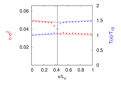
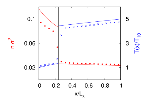
In Fig. 2, the steady temperature and density profiles are plotted for a system with $M/m=10$ and $T_{20}/T_{10}=1.5$. The profiles for a system with the same value of the mass ratio $M/m$, but with a much larger temperature ratio, $T_{20}/T_{10}=5$, are given in Fig. 3. The symbols are MD results, while the solid lines are the theoretical predictions obtained above. The vertical line indicates the average position of the piston. A fairly good agreement is observed. It is important to realize that the hydrodynamic fields in the vicinity of the average position of the piston are much influenced by the fluctuations of the latter, that are not accounted for in the simple model developed here.

Figure 2: Steady temperature (blue crosses and solid line) and density (red circles and solid line) profiles. The symbols are MD simulation results for a tow-dimensional system of $2N=200$ hard disks with $L_{x}=2S_{P}=100\sigma$, $M/m=10$, and $T_{20}/T_{10}=1.5$. The solid lines are the theoretical predictions derived in the main text.

Figure 3: The same as in Fig. 2, but now $T_{20}/T_{10}=5$

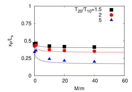
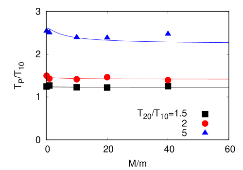
The results for the dependence of the steady position of the piston $x_{P}$ on the mass ratio $M/m$ are shown in Fig 4. Three different values of the ratio of the temperatures of both thermal wall have been considered, as indicated in the inset. As the mass ratio increases the position of the piston tends to a constant value. A similar behavior is observed for the temperature of the piston, shown in Fig. 5. In both cases, there is again a fairly good agreement between the simulation results and the theoretical prediction from the model proposed here.

Figure 4: Steady position of the piston $x_{P}$ as a function of the mass of the piston $M$. Three values of the ratio of the temperatures of the two thermal walls have been considered, as indicated. The values of $L_{x}$ and $N$ are the same as in Fig. 2. The symbols are MD simulation results while the solid lines are the predictions derived in the main text.

Figure 5: The same as in Fig 4, but now the plotted quantity is the temperature of the piston divided by the temperature of the cold wall.

It seems worth to investigate whether the steady state reached by the system considered here can be described by means of a minimum entropy production rule. The entropy production function $P$ of the system is [13, 14]

$$P = S_{P}\int_{0}^{x_{P}}dx\,q_{x1}(x)\frac{dT^{-1}_{1}(x)}{dx}$$ (26)

$$+S_{P}\int_{x_{P}}^{L_{x}}dx\,q_{x1}(x)\frac{dT_{2}^{-1}(x)}{dx}$$

$$-Q_{1}\left[\frac{1}{T_{P}}-\frac{1}{T_{1}(x_{P})}\right]$$

$$+Q_{2}\left[\frac{1}{T_{2}(x_{P})}-\frac{1}{T_{P}}\right],$$

where the possible discontinuity of the temperature at the piston has been taken into account. In this expression, the relations given in Eqs. (2), (9), (10), and (17) are assumed to be known since they correspond to boundary conditions. Moreover, the limit of small temperature gradients will be considered in the following. Define

$$T_{m}\equiv\frac{T_{10}+T_{20}}{2}\,,\quad\quad\theta\equiv\frac{T_{20}-T_{10}}{2T_{m}},$$ (27)

and introduce the scaled temperature deviations $\tau_{1}$, $\tau_{2}$, and $\tau_{P}$ by

$$T_{1}(x_{P})=T_{m}+\theta\tau_{1},\quad T_{2}(x_{P})=T_{m}+\theta\tau_{2},$$ (28)

$$\quad T_{P}=T_{m}+\theta\tau_{P}.$$ (29)

When these expressions are substituted into Eq. (26) and an expansion in powers of $\theta$ is carried out, it is obtained that

$$P(\tau_{1},\tau_{2},\tau_{3}) = \frac{6(2mk_{B})^{1/2}S_{P}}{\pi^{1/2}ML_{x}T_{m}^{3/2}}$$ (30)

$$\times\left\{2D\left[\tau_{1}^{2}+\tau_{2}^{2}-2\left(\tau_{1}+\tau_{2}\right)\tau_{P}+2\tau_{P}^{2}\right]\right.$$

$$+\left.C\left[\tau_{1}^{2}+\tau_{2}^{2}+2T_{m}(\tau_{1}-\tau_{2}+T_{m})\right]\right\}\theta^{2}$$

$$+\mathcal{O}(\theta^{4}).$$

The values of $\tau_{1}$, $\tau_{2}$ and $\tau_{3}$ minimizing this expression for small $\theta$, namely neglecting terms of order $\theta^{4}$ and higher, are

$$\tau_{1}=-\frac{CT_{m}}{C+2D}\,,\quad\tau_{2}=-\tau_{1},\quad\tau_{P}=0.$$ (31)

Using these values, it is easily seen that

$$x_{P}=\frac{L_{x}}{2}\left(1-\frac{C+D}{C+2D}\,\theta\right),\quad p=\frac{2Nk_{B}T_{m}}{L_{x}S_{P}}\,,$$ (32)

$$\quad a_{1}=a_{2}=\frac{6D}{C+2D}\frac{T_{m}^{3/2}\theta}{L_{x}}.$$ (33)

These results agree with the lowest order expansion in $\theta$ of Eqs. (23)-(25), as it can be easily verified. On the other hand, it is also easily seen that the condition that the entropy production $P$ is minimum is not equivalent to the hydrodynamic theory developed here outside of the limit of small temperature gradients, leading to results that strongly disagree with the numerical simulations.

In summary, it has been shown that the presence of the adiabatic piston introduces a strong discontinuity of the hydrodynamic profiles, increasing their slope in both compartments. Moreover. the simple model presented here based on the energy balance, reproduces quite well the molecular dynamics simulation results. A minimum entropy production requirement only holds in the limit of small temperature differences. Although we are not aware of any realization of a situation similar to the one considered here, the effects discussed should be observable in experiments, by extending the devices used to investigated the relaxation to equilibrium [15, 16, 17].

References

- [1] Callen H B 1963 Thermodynamics (New York: Wiley and Sons)
- [2] Feynman R P 1965 Lectures Notes in Physics (New York: Addison-Wesley)
- [3] Gruber Ch and Lesne A 2006 Encyclopedia of Mathematical Physics ed J P Francoise, G Naber and T S Tsun (Amsterdam: Elsevier) p 160
- [4] Brito R, Renne M J and Van der Broeck C 2005 Europhys. Lett. 70 29
- [5] Brey J J and Khalil N 2010 Phys. Rev. E 82 051301
- [6] Brey J J and Khalil N 2011 Europhys. Lett 94 14003
- [7] Dufty J W 2000 J. Phys.: Condens. Matter 12 A47
- [8] Goldhirsch I (2003) Annu. Rev. Fluid Mech. 35 267
- [9] Cercignani C 1969 Mathematical Methods in Kinetic Theory (New York: Plenum)
- [10] Dorfman J R and van Beijeren H 1997 Statistical Mechanics Part B ed B J Berne (New York: Plenum) p 65
- [11] Brey J J and Ruiz-Montero M J 2009 Phys. Rev. E 79 031305
- [12] Allen M P and Tisdesley D J 1987 Computer Simulation of Liquids (New York: Oxford Science Publications)
- [13] De Groot S R and Mazur P 1962 Non-Equilibrium Thermodynamics (Amsterdam: North-Holland)
- [14] McLennan J A 1989 Introduction to Non-Equilibrium Statistical Mechanics (London: Prentice Hall)
- [15] Rüchardt E 1929 Z. Phys. 30 58
- [16] Pierrus J and de Lange O L 1997 Phys. Rev. E 56 2841
- [17] de Langue O L and Pierrus J 1998 Phys. Rev. E 57 5520