Correlations between the dynamics of parallel tempering and the free-energy landscape in spin glasses

Abstract

We present the results of a large-scale numerical study of the equilibrium three-dimensional Edwards-Anderson Ising spin glass with Gaussian disorder. Using parallel tempering (replica exchange) Monte Carlo we measure various static, as well as dynamical quantities, such as the autocorrelation times and round-trip times for the parallel tempering Monte Carlo method. The correlation between static and dynamic observables for 5000 disorder realizations and up to 1000 spins down to temperatures at 20% of the critical temperature is examined. Our results show that autocorrelation times are directly correlated with the roughness of the free-energy landscape.

I Introduction

Systems in statistical physics with rough free-energy landscapes, such as spin glasses, are notoriously difficult to equilibrate using Markov chain Monte Carlo methods. The basic reason for this difficulty is that extremely long times are required to surmount free-energy barriers and, thus, to efficiently and fully explore the minima in the free-energy landscape. The parallel tempering algorithm (also known as “replica exchange Monte Carlo”) Geyer (1991); Marinari and Parisi (1992); Hukushima and Nemoto (1996), as well as other multicanonical techniques Janke, W. (1998); Berg (1999), have partially overcome this problem. However, there is little understanding of the relevant time scales for these methods. The purpose of this work is to shed light on the equilibration time of the parallel tempering algorithm and to understand how it is related to equilibrium properties such as the roughness of the free-energy landscape. To this end, we apply parallel tempering to a large ensemble of disorder realizations of the three-dimensional Edwards-Anderson (EA) Ising spin glass Edwards and Anderson (1975); Binder and Young (1986). Our main results are that equilibration times vary significantly from one disorder realization to another and that this variation is correlated with the structure of the free-energy landscape. The fact that equilibration times are broadly distributed has been previously noted in a different context (see, for example, Refs. Alder et al. (2004) and Alvarez Baños et al. (2010)) but the extent of variation was not fully appreciated because different measures of equilibration time were used in past studies. The correlation of dynamic time scales for parallel tempering and equilibrium properties has not been previously recognized, again because of the use of insensitive measures of dynamic time scales. In this study we compute autocorrelation functions of observables to measure equilibration times whereas previous studies have primarily relied on the round-trip time and related quantities. Although our study is focused on parallel tempering and the Edwards-Anderson Ising spin-glass model, we believe that our qualitative results are likely to be relevant both to other disordered systems with rough free-energy landscapes, as well as other multicanonical simulation techniques.

Parallel tempering was independently introduced by Geyer Geyer (1991) and Marinari and Parisi Marinari and Parisi (1992), as well as Hukushima and Nemoto Hukushima and Nemoto (1996). Furthermore, an earlier algorithm with many of the same essential features was introduced by Swendsen and Wang Swendsen and Wang (1986). In parallel tempering many copies of the system at different temperatures are simulated in parallel. Each copy (henceforth referred to as replica) is simulated using a standard, single-temperature Monte Carlo scheme such as the Metropolis or heat bath algorithms Krauth (2006). The set of temperatures is chosen so it includes both high temperatures (where rapid equilibration is possible using the single-temperature Monte Carlo method) and low temperatures of interest (where equilibration is not feasible using the standard algorithm). In addition to the single-temperature Monte Carlo moves, there are also replica exchange moves in which replicas at neighboring temperatures swap their temperatures. Replica exchange moves permit replicas to diffuse in temperature space Katzgraber et al. (2006a). The diffusion of replicas in temperature space permits an enormous speed-up relative to single-temperature Monte Carlo. Instead of directly surmounting the high free-energy barriers present at low temperatures, barriers are indirectly surmounted via the following process: A replica in one free-energy well at the lowest temperature diffuses to the highest temperature where it easily moves to another well and then diffuses back to the lowest temperature. This process is called a “round trip” and it allows parallel tempering to reduce exponential time scales for surmounting free-energy barriers to power-law time scales Machta (2009).

In the context of simple models with rough free-energy landscapes it has recently been shown Machta (2009) that the equilibration time of parallel tempering depends strongly on the structure of the free-energy landscape. If there is a single dominant minimum in the landscape and no first-order transition within the range of temperatures, then the equilibration time is short. On the other hand, the presence of several nearly degenerate minima or the existence of a first-order transition leads to much longer equilibration times. These results in simple model landscapes prompted us to look for similar phenomena in the Edwards-Anderson model where different disorder realizations may have quite different free-energy landscapes. In this study, rather than measuring the free-energy landscape directly, we used the spin overlap (order parameter) distribution as a proxy. The overlap distribution is closely related to the free-energy landscape but is substantially easier to measure in simulations. Based on the results from simple model free-energy landscapes, we hypothesize that when the overlap distribution has a complex structure, implying many free-energy minima the time scale for parallel tempering will tend to be longer than when the overlap distribution is simple. Our results confirm this hypothesis.

This study is part of a larger project whose goal is to understand the nature of the low-temperature phase of finite-dimensional spin glasses. The low-temperature phase of the Edwards-Anderson model is poorly understood and hotly debated. There are several competing theories for the low-temperature behavior of the model Fisher and Huse (1986, 1988); Parisi (1979); Mézard et al. (1987); Marinari et al. (1998); Newman and Stein (1996, 1998); Krzakala and Martin (2000); Palassini and Young (2000); Katzgraber et al. (2001) and even though many large-scale investigations have been conducted Palassini and Young (2000); Katzgraber et al. (2001); Katzgraber and Young (2002); Katzgraber et al. (2006b); Alvarez Baños et al. (2010), a conclusive theory correctly explaining all phenomena has not been agreed on. Our recent simulations Yucesoy et al. (2012) point toward a two-pure-state picture such as the droplet picture McMillan (1984); Fisher and Huse (1986, 1987, 1988); Bray and Moore (1986) or the chaotic pairs picture Newman and Stein (1992, 1996, 1998). One motivation for this work was to verify that the ensemble of disorder realizations used in Ref. Yucesoy et al. (2012) was indeed equilibrated. Therefore, we have measured both equilibration times and overlap distributions for all disorder realizations and correlated these quantities. We also demonstrate that the conservative use of the equilibration criterion introduced in Ref. Katzgraber et al. (2001) is sufficient to ensure that nearly all disorder samples are equilibrated.

Our results suggest both a method for improving parallel tempering and a warning when using it in spin-glass simulations. On the one hand, we find that many disorder realizations have quite short equilibration times. Thus it might be useful to implement an adaptive scheme where some disorder realization are simulated for shorter times than other realizations. State-of-the-art parallel tempering simulations of equilibrium spin glasses require huge amounts of CPU time because of the difficulty of reaching equilibrium and the need for a large ensemble of disorder realizations. Thus, such an adaptive scheme has the potential for large savings in CPU time. On the other hand, the fact that the overlap distribution (a quantity directly related to the controversy surrounding the low-temperature phase of spin glasses) is significantly correlated with the dynamics of the algorithm serves as a warning that one must be extremely careful to ensure that essentially all samples are well equilibrated in order to avoid systematic errors in measuring disordered-averaged equilibrium properties.

The paper is organized as follows: In Sec. II we introduce the model, the parallel tempering algorithm, as well as the measured observables. In Sec. III we show our results, followed by conclusions.

II Model and Methods

II.1 The Edwards-Anderson Ising spin glass

We study the three-dimensional EA Ising spin-glass model, defined by the energy function

$$H=-\sum_{\langle i,j\rangle}J_{ij}s_{i}s_{j}.$$ (1)

The sum is over the nearest neighbors on a simple cubic lattice with periodic boundary conditions and side length $L$. The Ising spins $s_{i}$ take values $\pm 1$ and the interactions $J_{ij}$ are quenched random couplings chosen from a Gaussian distribution with zero mean and unit variance.

II.2 Parallel tempering Monte Carlo

Parallel tempering, also known as replica exchange Monte Carlo, is a powerful tool for simulating systems with rough free-energy landscapes Earl and Deem (2005); Katzgraber et al. (2006a); Machta (2009) with applications across many disciplines. To date, it is the most efficient method for simulating spin glasses and other disordered systems in more than two dimensions at low temperatures where dynamics are slow.

The algorithm works as follows: Several copies (hereafter also referred to as replicas) of the system with the same disorder are simulated in parallel. Each replica is simulated at a different temperature using a standard Markov chain Monte Carlo (MCMC) technique such as the Metropolis or heat-bath algorithms Newman and Barkema (1999); Krauth (2006); Katzgraber (2009). In this work we use the heat bath algorithm because of its better performance at low temperature. The set of temperatures is chosen to span both the low temperatures of interest, where equilibration is not feasible using single-temperature MCMC methods, and high temperatures where equilibration is fast. In addition to the MCMC sweeps of each temperature, there are also replica exchange moves between replicas. A proposed replica exchange move involves swapping the temperatures of two replicas at neighboring temperatures. A replica exchange move is accepted with probability $p$, where

$$p=\min[1,e^{(\beta-\beta^{\prime})(E-E^{\prime})}].$$ (2)

Here $\beta=1/T$ is the inverse temperature of one replica and $\beta^{\prime}$ the inverse temperature of the neighboring replica, and $E$ and $E^{\prime}$ are the corresponding energies of the two replicas. Equation (2) ensures that the entire Markov chain, including both single-temperature MCMC sweeps and replica exchange moves satisfies detailed balance and converges to equilibrium. Replica exchange allows replicas to diffuse from the lowest temperature to the highest temperature and back again. These round trips enhance mixing and greatly reduce equilibration times for rough energy landscapes.

The parallel tempering algorithm has free parameters that include the set of temperatures and the ratio of single-temperature sweeps to replica-exchange sweeps. Optimizing parallel tempering therefore requires an appropriate choice of these parameters. The choice of the number of replicas $N_{T}$ and their temperatures involves the following trade-off: If there are many closely-spaced temperatures, the energy distribution between adjacent temperatures overlaps strongly and the probability that a proposed replica exchange is accepted, see Eq. (2), is large. This suggests that the more replicas one uses, the better, apart from the extra computational work involved in carrying out single-temperature sweeps of each replica. However, the motion of replicas in temperature space is diffusive such that the time scale for a round-trip scales approximately as the square of the number of temperatures. At least for simple model systems, parallel tempering is optimized if the number of temperatures scales as the square root of the number of spins Machta (2009). The average time to complete one round trip is often used to characterize the performance of parallel tempering. Choosing a set of temperatures that minimizes the round trip time is one of the ways proposed to optimize parallel tempering Katzgraber et al. (2006a); Trebst et al. (2006); Bittner et al. (2008); Hasenbusch and Schaefer (2010).

II.3 Simulation parameters

For the parallel tempering algorithm we use $N_{T}=16$ temperatures between $T=0.2$ to $2.0$ com (a). This set of temperatures was chosen heuristically in Refs. Katzgraber et al. (2001) and Katzgraber and Young (2002) to perform well for $L=6$ and $8$. The corresponding average acceptance fractions for replica exchange moves are plotted in Fig. 1. It is likely that the simulations would be more efficient if more replicas were used near and above the critical region ($T_{c}\approx 0.96$ Katzgraber et al. (2006b)) where the acceptance fractions are small. However, we believe that as long as the swapping probability is nonzero, our results will not change qualitatively. A bottleneck merely slows down the diffusion process but does not prevent it. For $L=10$, the small acceptance fractions suggest that a larger number of temperatures might be more efficient. However, our goal is to understand correlations between static and dynamic quantities in parallel tempering for a given system size and so we have not sought to optimize the algorithm for each system size. We believe that the qualitative results obtained using our parallel tempering parameters would also hold for other reasonable values of the parameters.

Figure 1: (Color online) Average acceptance fraction as a function of temperature $T$ for replica exchange moves. Note that $T_{c}\approx 0.96$.

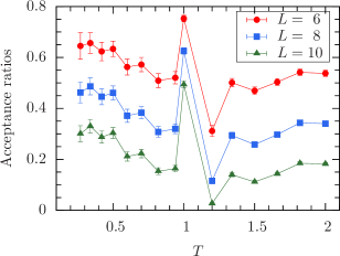
By placing the hottest system temperature at $T\approx 2T_{c}$, we ensure that equilibration happens quickly, and we use one exchange sweep for each heat-bath sweep ($N=L^{3}$ attempted spin updates). To calculate the spin overlap [Eq. (3)] we use two copies of the system at each temperature; therefore, for each sample, we simulate two sets of replicas independently from each other.

As stated before, we employ one replica exchange sweep after one heat-bath sweep. A heat-bath sweep corresponds to sequentially attempting to update each spin at each replica once using the heat-bath algorithm. An exchange sweep corresponds to randomly choosing $N_{T}-1$ pairs of adjacent replicas and proposing exchanges for each. Both types of sweeps together make up one parallel tempering sweep. When no confusion arises, we will call this unit of time simply a sweep.

For each system size we simulate approximately $5000$ disorder realizations or samples. The simulations are equilibrated for at least $2^{24}$ sweeps for $L=6$ and $2^{27}$ sweeps for $L=8$ and $10$, and then measurements are done for the same number of sweeps; see Table 1 for details. A fraction of samples required longer runs to meet the equilibration criteria discussed in Sec. II.4.2. For samples with very short equilibration times, we performed runs to obtain fine-grained autocorrelation information; see Sec. II.4.2. In total, the data collection took approximately 140 CPU years on 12-core AMD Opteron 6174 CPUs.

Table 1: For each system size $L$ we equilibrate and then measure for at least $2^{b}$ Monte Carlo sweeps. $T_{\rm min}$ ($T_{\rm max}$) is the lowest (highest) temperature used, $N_{T}$ is the number of temperatures, and $N_{\rm sa}$ is the number of disorder realizations. For some $L=10$ samples longer runs had to be performed to ensure equilibration.

$L$	$b$	$T_{\rm min}$	$T_{\rm max}$	$N_{T}$	$N_{\rm sa}$
$6$	$24$	$0.2$	$2.0$	$16$	$4961$
$8$	$27$	$0.2$	$2.0$	$16$	$5126$
$8$	$28$	$0.2$	$2.0$	$16$	$4$
$10$	$27$	$0.2$	$2.0$	$16$	$4360$
$10$	$28$	$0.2$	$2.0$	$16$	$353$
$10$	$29$	$0.2$	$2.0$	$16$	$241$
$10$	$30$	$0.2$	$2.0$	$16$	$73$

II.4 Observables

II.4.1 Overlap distributions

The focus of the paper is to relate static equilibrium properties of individual spin-glass samples to the dynamics of the parallel tempering algorithm acting on that sample. The primary quantity that we measure to study both equilibrium properties and the dynamics of parallel tempering is the spin overlap $q$,

$$q=\frac{1}{N}\sum^{N}_{i=0}s_{i}^{(1)}s_{i}^{(2)},$$ (3)

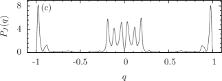
where $N=L^{3}$ is the number of spins and the superscripts $(1)$ and $(2)$ indicate two independent copies of the system with the same disorder. The thermal and disorder average of the overlap is an order parameter for the system and the probability distribution of the thermally averaged overlap $P_{J}(q)$ for a given sample $J$ reveals aspects of the free-energy landscape for that particular sample. The behavior of $P_{J}(q)$ for large systems and at low temperatures is one of the major open questions in the theory of spin glasses. Overlap distributions vary widely from sample to sample, as can be seen in the three examples shown in Fig. 2. Although there is no direct mapping between the free-energy landscape and $P_{J}(q)$, it is clear that numerous peaks in $P_{J}(q)$ imply numerous minima in the free-energy landscape. For example, samples corresponding to Figs. 2(b) and 2(c) have a more complicated free-energy landscapes than Fig. 2(a). Our central hypothesis is that samples with a more complicated free-energy landscape tend to have longer dynamic time scales.

Figure 2: Examples of overlap distributions $P_{J}(q)$ for three different disorder realizations $J$ for $L=8$. While the distribution in panel (a) has only two peaks, the distribution in panel (c) implies a very complex free-energy landscape. All panels have the same horizontal scale.

From $P_{J}(q)$ we define $I_{J}(q_{0})$ for different $q_{0}$,

$$I_{J}(q_{0})=\int_{-q_{0}}^{q_{0}}P_{J}(q),$$ (4)

where $I_{J}(q_{0})$ is the weight of $P_{J}(q)$ in an interval near the origin and it serves as an approximate measure of the complexity of $P_{J}(q)$. For example, $I_{J}(0.2)\approx 0$ for the samples shown in Figs. 2(a) and 2(b), while $I_{J}(0.2)$ is large for the sample shown in Fig. 2(c). We compute $I_{J}(q_{0})$ for eight values of $q_{0}$ from $q_{0}=0.2$ to $0.9$. It is worth noting that $I_{J}(q_{0})$—especially with $q_{0}=0.2$—has been extensively used in studies of the low-temperature equilibrium properties of the EA model Katzgraber et al. (2001); Alvarez Baños et al. (2010).

II.4.2 Characteristic time scales

We measure two time scales for parallel tempering from the autocorrelation function of the overlap at the lowest temperatures. For an arbitrary observable ${\cal A}$, the autocorrelation function $\Gamma_{{\cal A}}(t)$ is defined via

$$\Gamma_{{\cal A}}(t)=\frac{\langle{\cal A}(0){\cal A}(t)\rangle-\langle{\cal A}\rangle^{2}}{\langle{\cal A}^{2}\rangle-\langle{\cal A}\rangle^{2}}.$$ (5)

Here, ${\cal A}(t)$ is the observable measured at time $t$ and $\langle\cdots\rangle$ represents a thermal average com (b). Integrated and exponential autocorrelation times are computed from the autocorrelation function. The integrated autocorrelation time $\tau^{\cal A}_{\rm{int}}$ is the integral of the autocorrelation function or, for discrete time, the sum of the autocorrelation function,

$$\tau^{\cal A}_{\rm{int}}=\frac{1}{2}+\displaystyle\sum_{t=1}^{\infty}\Gamma_{{\cal A}}(t).$$ (6)

The integrated autocorrelation time is the time needed for two subsequent measurements of ${\cal A}$ to decorrelate. It is a lower bound on the time needed to reach equilibrium from an arbitrary initial condition. To calculate $\tau^{\cal A}_{\rm{int}}$ care must be taken when truncating the sum in Eq. (6) to avoid large statistical errors (explained below).

Figure 3 shows two typical examples of the autocorrelation function for the absolute value of the spin overlap $|q|$. For large times, the autocorrelation function is eventually dominated by noise. The noise floor is indicated in Figs. 3 by the horizontal (red) solid line. Because the noise floor is determined primarily by the number of data points used to compute the autocorrelation function, it can be chosen to be the same for all simulations of the same length. Our truncation procedure is to sum the autocorrelation function until it first hits the noise floor. We obtain the noise floor for each run length by visual inspection of $\Gamma_{|q|}(t)$ for many samples. We note that this approach introduces some slight systematic bias in our estimates of the integrated autocorrelation times. However, the main emphasis of this paper is to understand the very large sample-to-sample variations in time scales and, compared to these variations, the errors introduced by our truncation protocol are small.

Figure 3: (Color online) Autocorrelation function for the absolute value of the order parameter $\Gamma_{|q|}(t)$ as a function of simulation time for two different disorder realizations and system size $L=8$. The horizontal (red) solid line at $\Gamma_{|q|}=0.005$ represents the noise floor. The diagonal solid (green) lines represent exponential fits to the data. Both panels have the same horizontal scale.

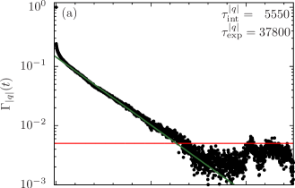
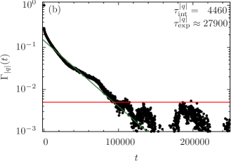
We have computed autocorrelation functions for both $|q|$ and $q$ and from these we have obtained $\tau^{|q|}_{\rm{int}}$ and $\tau^{q}_{\rm{int}}$, respectively. To do this, we first compute a Fourier transform of the data and then invert the function to obtain the autocorrelation function. This method is considerably faster than a direct calculation. For $L=6$, the simulations are run for $2^{24}$ sweeps, recording data for the computation of the autocorrelation functions every $10$ sweeps. The noise floor for these runs is set to $\Gamma=0.005$. Some samples have $\tau^{|q|}_{\rm{int}}$ values of order 10 or less. For these, shorter data collection runs of $2^{18}$ sweeps have been done starting from an equilibrated spin configuration stored at the end of the longer run. For these short runs data are collected every sweep to accurately measure the autocorrelation function up to time 10 and the full autocorrelation function is patched together from the short and long runs. The noise floor for these shorter runs is set to $\Gamma=0.01$. If the noise floor is reached before $t=10$, only the autocorrelation function generated by the short run is used. For both $L=8$ and $L=10$ the simulations are run for at least $2^{27}$ sweeps, recording data every $100$ sweeps with shorter runs also needed for samples with small $\tau^{|q|}_{\rm{int}}$ values. The noise floor used is the same as for $L=6$.

The autocorrelation function is always calculated up to a maximum time lag of 1% of the total run length. Therefore, for some samples and, in particular for $L=10$, the noise floor was not reached by this time and longer runs were necessary to obtain good statistics. For these $L=10$ samples we simulate up to $2^{30}$ sweeps. 32 samples (approximately $0.6\%$) stayed above the noise floor even for the longest runs. To prevent a biasing of the results, these were not included in the analysis. However, it would be interesting to study these samples in detail in the future.

There is another method for truncating the sum in Eq. (6) introduced by Madras and Sokal Madras and Sokal (1988) where the upper limit of the sum is determined recursively. An initial upper limit is chosen and $\tau^{\cal A}_{\rm{int}}$ is computed for that value, and the new upper limit is determined as some factor ($6$ is suggested in Ref. Madras and Sokal (1988)) times the current $\tau^{\cal A}_{\rm{int}}$. The estimated value of $\tau^{\cal A}_{\rm{int}}$ is obtained when this process has converged. We experimented with this approach but did not find that it converged in a consistent way across all samples with very different autocorrelation functions. However, we note that our approach should have systematic errors no larger than those resulting from the method of Madras and Sokal with the upper limit set to $6\tau^{|q|}_{\rm{int}}$ because the noise floor is not reached until at least $10\tau^{|q|}_{\rm{int}}$ except for the very few samples with extremely small $\tau^{|q|}_{\rm{int}}$ values.

The second time scale that we consider is the exponential autocorrelation time $\tau^{\cal A}_{\rm{exp}}$, defined by the asymptotic exponential decay of the autocorrelation function,

$$\Gamma_{{\cal A}}(t)\sim Ae^{-t/\tau^{\cal A}_{\rm{exp}}}.$$ (7)

Except for observables orthogonal to the slowest mode of the Markov chain, $\tau^{\cal A}_{\rm{exp}}$ is the characteristic time of the slowest mode and is thus the exponential time scale to reach equilibrium from an arbitrary initial state Sokal (1989).

In principle, $\tau^{\cal A}_{\rm{exp}}$ is the most important time scale for studying disordered systems because the main difficulty is reaching thermal equilibrium (controlled by $\tau^{\cal A}_{\rm{exp}}$) rather than collecting enough uncorrelated data at equilibrium (controlled by $\tau^{\cal A}_{\rm{int}}$). Unfortunately, calculating $\tau^{\cal A}_{\rm{exp}}$ for a large number of samples is difficult because it requires an automatized fitting process. For some samples, such as the one shown in Fig. 3, the autocorrelation function decays nearly exponentially over most of the observable time range, allowing for a precise fitting and extraction of $\tau^{|q|}_{\rm{int}}$. However, for many samples the autocorrelation function is not exponential for the measured times, as can be seen in Fig. 3 and, for these samples, an automatic fitting procedure would not be reliable. For that reason, the time scale that we correlate with the static properties of the EA spin glass is the integrated autocorrelation time. We have studied $\tau^{|q|}_{\rm{exp}}$ by hand for a small subset of the data set and find that for those samples where a reasonable fit is possible, $\tau^{|q|}_{\rm{exp}}$ is in the range of $1$ to $15$ times $\tau^{|q|}_{\rm{int}}$. Most, but not all, samples share the behavior seen in the examples in Figs. 3 that there is an initial sharp decline before the (approximately) exponential decay sets in. This sharp decline explains why $\tau^{|q|}_{\rm{exp}}$ is typically larger than $\tau^{|q|}_{\rm{int}}$.

Finally, we also measured the round-trip time $\tau_{\rm{RT}}$ for each sample, defined as the average time after equilibration is achieved, for a replica to diffuse from the lowest to the highest temperature and then back to the lowest temperature again Katzgraber et al. (2006a).

III Results

Figure 4: Logarithmic histogram of the integrated autocorrelation times $\tau^{|q|}_{\rm{int}}$ for for $L=8$. The data are normally distributed and show that a small fraction of samples is extremely difficult to equilibrate.

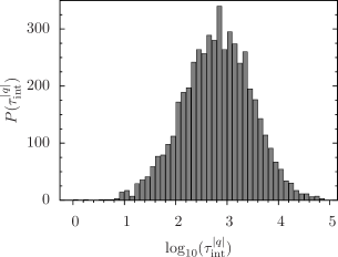
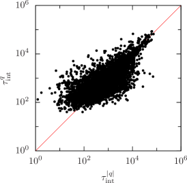
Figure 4 shows the probability distribution for $\tau^{|q|}_{\rm{int}}$ for $L=8$. In agreement with previous studies Alder et al. (2004); Katzgraber et al. (2006b); Alvarez Baños et al. (2010), the figure reveals that the equilibration times for spin glasses are very broadly distributed. The distributions for $L=6$ and $10$ are similar although with different logarithmic means and standard deviations, as shown in Tables 3 and 3, respectively. Tables 3 and 3 also show the logarithmic mean and standard deviation of $\tau^{q}_{\rm{int}}$. The values for $\tau^{q}_{\rm{int}}$ are similar to those for $\tau^{|q|}_{\rm{int}}$, however, the standard deviations are somewhat smaller. Figure 5 shows a scatter plot with each point representing one sample for $L=8$. The $x$ and $y$ coordinates are determined by $\tau^{q}_{\rm{int}}$ and $\tau^{|q|}_{\rm{int}}$, respectively. The data illustrate that $\tau^{q}_{\rm{int}}$ and $\tau^{|q|}_{\rm{int}}$ are strongly correlated, especially for those samples with the longest integrated autocorrelation times. The observation that $\tau^{|q|}_{\rm{int}}$ can take smaller values than $\tau^{q}_{\rm{int}}$ is presumably a consequence of the fact that the decorrelation of $q$ requires global spin flips while the decorrelation of $|q|$ does not.

Figure 5: (Color online) Scatter plot of $\tau^{q}_{\rm{int}}$ vs. $\tau^{|q|}_{\rm{int}}$ for $L=8$. The diagonal (red) solid line corresponds to $\tau^{q}_{\rm{int}}=\tau^{|q|}_{\rm{int}}$. Note that $\tau^{|q|}_{\rm{int}}$ is often smaller than $\tau^{q}_{\rm{int}}$ because the decorrelation of $q$ requires global spin flips while the decorrelation of $|q|$ does not.

Table 2: Mean values of the logarithms of $\tau^{q}_{\rm{int}}$, $\tau^{|q|}_{\rm{int}}$ and $\tau_{\rm{RT}}$ for system sizes $L=6$ – $10$.

$L$	$6$	$8$	$10$
$\log_{10}(\tau^{q}_{\rm{int}})$	$1.7164(58)$	$2.8366(75)$	$3.8711(84)$
$\log_{10}(\tau^{|q|}_{\rm{int}})$	$1.6035(90)$	$2.8065(94)$	$3.8881(97)$
$\log_{10}(\tau_{\rm{RT}})$	$3.6217(28)$	$4.4571(34)$	$5.2421(42)$

Table 3: Standard deviations of the logarithms of $\tau^{q}_{\rm{int}}$, $\tau^{|q|}_{\rm{int}}$ and $\tau_{\rm{RT}}$ for system sizes $L=6$ – $10$.

$L$	$6$	$8$	$10$
$\log_{10}(\tau^{q}_{\rm{int}})$	$0.408$	$0.534$	$0.592$
$\log_{10}(\tau^{|q|}_{\rm{int}})$	$0.631$	$0.672$	$0.685$
$\log_{10}(\tau_{\rm{RT}})$	$0.194$	$0.242$	$0.293$

Figures 6(a) and 6(b) show scatter plots of $\tau^{|q|}_{\rm{int}}$ vs $I_{J}(q_{0})$ for $L=8$ and $q_{0}=0.2$ and $q_{0}=0.8$, respectively. Each point represents one sample. These figures show that $\tau^{|q|}_{\rm{int}}$ is correlated with $I_{J}(q_{0})$ and the correlation is stronger for larger values of $q_{0}$. It is also striking that large values of $I_{J}(q_{0})$ are never associated with very small integrated autocorrelation times (similar results are obtained for the other system sizes studied). This suggest that when the free-energy landscape is complex, time-scales are large, as one would naively expect.

Figure 6: Scatter plot for all $L=8$ samples of $\tau^{|q|}_{\rm{int}}$ vs $I_{J}(q_{0})$ for (a) $q_{0}=0.2$ and (b) $q_{0}=0.8$. The empty area underneath the scatter for large $I_{J}(q_{0})$ clearly shows that realizations with large values of $I_{J}(q_{0})$ can never have small values of $\tau^{|q|}_{\rm{int}}$.

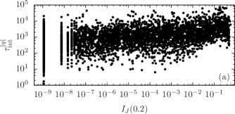
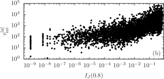
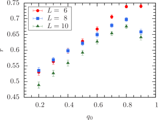
To quantify the correlations between $\tau^{|q|}_{\rm{int}}$ and $I_{J}(q_{0})$, we use the Pearson correlation coefficient $r$ Press et al. (1995), whose estimator for a finite data set $\{(x_{i},y_{i})\}$ is

$$r=\frac{\displaystyle\sum_{i=0}^{M}(x_{i}-\bar{x})(y_{i}-\bar{y})}{\sqrt{\displaystyle\sum_{i=0}^{M}(x_{i}-\bar{x})^{2}\displaystyle\sum_{i=0}^{M}(y_{i}-\bar{y})^{2}}},$$ (8)

where $M$ is the size of the data set and the overbar indicates the average over the data set. If $r=1$ there is an exact linear relationship between $x$ and $y$ while a small value of $r$ indicates the absence of any linear dependence. Pearson $r$ values for $\log_{10}(\tau^{|q|}_{\rm{int}})$ vs $\log_{10}[I_{J}(q_{0})]$ for our data are shown in Table 4 and Fig. 7 for the system sizes studied and different values of $q_{0}$. These results clearly demonstrate that longer parallel tempering time scales are correlated with more complicated overlap distributions. The strength of the correlation is slightly weaker for larger systems. The fact that $r$ increases with $q_{0}$ suggests that the presence of additional peaks in $P_{J}(q)$ increases $\tau^{|q|}_{\rm{int}}$ independent of whether those peaks are near the origin.

Figure 7: (Color online) Pearson correlation $r$ between $\log_{10}[I_{J}(q_{0})]$ and $\log_{10}(\tau^{|q|}_{\rm{int}})$ vs $q_{0}$. The data suggest that longer parallel tempering time scales are correlated with more complicated overlap distributions.

Table 4: Pearson correlation $r$ between the overlap weight $\log_{10}[I_{J}(q_{0})]$ for various $q_{0}$ and the logarithm of the integrated autocorrelation time for the overlap $\log_{10}(\tau^{|q|}_{\rm{int}})$ for the three system sizes, $L$. The bottom row shows the correlation coefficient between the logarithm of the round trip time $\log_{10}(\tau_{\rm{RT}})$ and $\log_{10}(\tau^{|q|}_{\rm{int}})$.

$q_{0}$	$L=6$	$L=8$	$L=10$
$0.2$	$0.5299(94)$	$0.5355(95)$	$0.4889(95)$
$0.3$	$0.5634(86)$	$0.5693(79)$	$0.5264(93)$
$0.4$	$0.5982(80)$	$0.5983(75)$	$0.5590(91)$
$0.5$	$0.6286(77)$	$0.6217(73)$	$0.5920(80)$
$0.6$	$0.6671(72)$	$0.6494(70)$	$0.6272(72)$
$0.7$	$0.7062(63)$	$0.6788(66)$	$0.6535(65)$
$0.8$	$0.7385(46)$	$0.6975(63)$	$0.6752(57)$
$0.9$	$0.7397(58)$	$0.6583(85)$	$0.6410(83)$
$\log_{10}(\tau_{\rm{RT}})$	$0.014(19)$	$0.114(17)$	$0.126(20)$

Figure 8: (Color online) Scatter plot of the average round trip time $\tau_{\rm{RT}}$ vs $\tau^{|q|}_{\rm{int}}$ for $L=8$. The diagonal (red) line is $\tau_{\rm{RT}}=\tau^{|q|}_{\rm{int}}$. The data show almost no correlation between these quantities.

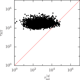
On the other hand, we find that the round trip time is not correlated with $\tau^{|q|}_{\rm{int}}$ or, by extension, $I_{J}(q_{0})$. Figure 8 is a scatter plot of $\tau_{\rm{RT}}$ vs $\tau^{|q|}_{\rm{int}}$ for $L=8$ (compare with Fig. 5). Each point represents one sample and the diagonal line is $\tau_{\rm{RT}}=\tau^{|q|}_{\rm{int}}$. It is clear from this figure that $\tau_{\rm{RT}}$ has a much smaller variance than $\tau^{|q|}_{\rm{int}}$ and that the correlation between the two is minimal. The last row of Table 4 shows the Pearson $r$ value between $\log_{10}(\tau_{\rm{RT}})$ and $\log_{10}(\tau^{|q|}_{\rm{int}})$ and quantifies the lack of correlation between $\tau_{\rm{RT}}$ and $\tau^{|q|}_{\rm{int}}$. Note that the authors of Ref. Alvarez Baños et al. (2010) consider a time scale related to the motion of replicas in parallel tempering and also find no correlation with $I_{J}(q_{0})$.

If the highest temperature is chosen such that its mixing time is one heat bath sweep, then $\tau_{\rm{RT}}\geq\tau^{|q|}_{\rm{int}}$ because there will be no memory of the spin state of the replica between successive visits to the lowest temperature, as can be seen in Tables 3 and 3, as well as Fig. 8. Figure 8 shows that $\tau_{\rm{RT}}$ is much larger than $\tau^{|q|}_{\rm{int}}$ for most samples. One explanation for this is that (for most samples) the spin state of the coldest replica can be decorrelated by diffusion from the lowest temperature to an intermediate temperature and back; full round trips are not needed for decorrelation.

Note that if we repeat the study for $\tau^{q}_{\rm{int}}$ instead of $\tau^{|q|}_{\rm{int}}$, the correlation values would show the same qualitative trend as for $\tau^{|q|}_{\rm{int}}$, but they would, on average, be slightly smaller.

Finally, we also test equilibration with the method introduced by Katzgraber et al. in Ref. Katzgraber et al. (2001) for short-range spin glasses with Gaussian disorder between the spins. In this method, the average energy per spin

$$u=-\frac{1}{N}\sum_{\langle i,j\rangle}[\,J_{ij}\langle s_{i}s_{j}\rangle\,]_{\rm av},$$ (9)

where $[\cdots]_{\rm av}$ represents a disorder average and, as before, $\langle\cdots\rangle$ denotes the Monte Carlo average for a given set of bonds, can be related to the link overlap

$$q_{l}=\frac{1}{N_{b}}\sum_{\langle i,j\rangle}s_{i}^{(1)}s_{j}^{(1)}s_{i}^{(2)}s_{j}^{(2)}$$ (10)

via an integration by parts over the interactions $J_{ij}$ between the spins. In Eq. (10) $N_{b}=dN$ with $d=3$ the space dimension represents the number of bonds in the system. One obtains:

$$[\langle q_{l}\rangle]_{\rm av}=1-\frac{T|u|}{d},$$ (11)

where $T$ is the temperature.

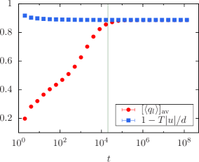
Figure 9 shows representative results for $L=8$ and $T=0.2$, the lowest temperature simulated. At approximately $10^{5}$ Monte Carlo sweeps both data computed directly from the energy per spin (blue squares) and data computed from the link overlap (red circles) agree within error bars. Note that 99% of the $\tau^{|q|}_{\rm{int}}$ values for this system size are smaller than the point marked with the solid vertical (green) line in Fig. 9. Thus, for the simulated time of over $10^{8}$ Monte Carlos sweeps, the data are well equilibrated. This suggests that a conservative use of the equilibration criterion developed in Ref. Katzgraber et al. (2001) will guarantee that almost all of the samples are equilibrated.

Figure 9: (Color online) Average link overlap $[\langle q_{l}\rangle]_{\rm av}$ (red circles) and $1-T|u|/d$ [see Eq. (11), blue squares] as a function of time $t$ for $L=8$ and $T=0.20$. For $t\gtrsim 10^{5}$ sweeps both data sets agree, suggesting that the system is in thermal equilibrium. The vertical (green) line in the figure represents the time for which 99% of the samples have values of $\tau^{|q|}_{\rm{int}}$ less than this time. Error bars are smaller than the symbols.

IV Conclusions

We have found one factor that explains the broad distribution of time scales in parallel tempering for spin glasses: The roughness of the free-energy landscape of each individual sample directly affects its equilibration time scales. In accordance with previous observations on the parallel tempering method Machta (2009), if there are many minima in the free-energy landscape, a sample requires more time to equilibrate. The equilibrium distribution of the spin overlap serves as proxy for the complexity of the free-energy landscape. Our results show that individual samples need to be tested individually to ensure proper equilibration, as previously suggested in Ref. Alvarez Baños et al. (2010). However, we show that the equilibration test developed in Ref. Katzgraber et al. (2001) is a viable alternative for system sizes currently accessible in simulations if applied conservatively. Furthermore, the parallel tempering round-trip times seem to be unaffected by the complexity of the free-energy landscape and should therefore not be used as a measure of how well a system is equilibrated.

The clear correlations between algorithmic (nonequilibrium) time scales and the equilibrium complexity of the free-energy landscape opens the door for alternate studies of the nature of the spin-glass state, a problem that remains controversial.