Peccei-Quinn symmetry as the origin of Dirac Neutrino Masses

Abstract

We propose a model of Dirac neutrino masses generated at one-loop level. The origin of this mass is induced from Peccei-Quinn symmetry breaking which was proposed to solve the so-called strong CP problem in QCD, therefore, the neutrino mass is connected with the QCD scale, $\Lambda_{\rm QCD}$. We also study the parameter space of this model confronting with neutrino oscillation data and leptonic rare decays. The phenomenological implications to leptonic flavor physics such as the electromagnetic moment of charged leptons and neutrinos are studied. Axion as the dark matter candidate is one of the byproduct in our scenario. Di-photon and Z-photon decay channels in the LHC Higgs search are investigated. We show that the effects of singly charged singlet scalar can be distinguished from the general two Higgs doublet model.

I Introduction

Small quantities arising in physics usually requires the use of new symmetries for explanations t'hooft . A good example of these is the Peccei-Quinn (PQ) symmetry that plays the role for the solution of the strong CP-problem Peccei:1977hh ; Peccei:1977ur , in which a $\theta$-angle appears in the QCD lagrangian, $\mathcal{L}_{QCD}\in\theta\frac{g^{2}_{S}}{32\pi^{2}}G^{a}_{\mu\nu}\tilde{G}^{a\mu\nu}$, and CP is violated 'tHooft:1976up ; Jackiw:1976pf ; Callan:1976je . The instanton solution to the gluon field equations satisfies $n=\frac{1}{32\pi^{2}}\int d^{4}xG^{a}_{\mu\nu}\tilde{G}^{a\mu\nu}$ with $n$’s being integers and representing topological charges Belavin:1975fg . The QCD vacuum state hence can be parametrized as $|\theta\rangle=\sum_{n=-\infty}^{n=\infty}e^{in\theta}|n\rangle$ where $\theta$ is periodic with period $2\pi$. Furthermore for nonzero quark masses the chiral anomaly relates the weak phase in quark masses to the QCD $\theta$-term. One can parametrize the $\theta$ angle as $\bar{\theta}=\theta-{arg}\{{\rm{det}}m_{q}\}$ Adler:1969gk ; Bell:1969ts . It induces a neutron electric dipole moment (EDM) Baluni:1978rf ; Crewther:1979pi ; Cea:1984qv ; Schnitzer:1983pb ; Musakhanov:1984qy and the current experimental upper bound set the best constraint on $\bar{\theta}$ to be smaller than $0.6\times 10^{-10}$ Baker:2006ts . This extremely suppressed quantity is called the strong CP problem. The Peccei-Quinn solution to the strong CP problem postulates a global chiral $U(1)_{PQ}$ symmetry and makes $\bar{\theta}$ a dynamical variable, and the shift symmetry of the Nambu-Goldstone boson, axion, corresponding to $U(1)_{PQ}$ Weinberg:1977ma ; Wilczek:1977pj will set $\bar{\theta}$ zero at classical potential Vafa:1984xg . At one-loop level the chiral anomaly will break the shift symmetry. As a result the axion is not massless but requires a small mass $m_{a}\simeq\frac{\sqrt{m_{u}m_{d}}}{(m_{u}+m_{d})}\frac{f_{\pi}m_{\pi}}{f_{a}}\sim\frac{\Lambda^{2}_{QCD}}{f_{a}}$ Peccei:2006as ; Kim:1986ax ; Cheng:1987gp . Here $f_{a}$ is the $U(1)_{PQ}$ breaking scale and $f_{\pi}$ is the pion decay constant. The laboratory pdg and outer space Andriamonje:2007ew ; Arik:2011rx ; Inoue:2008zp ; Asztalos:2006kz ; Asztalos:2009yp searches have set $10^{9}~{}{\rm GeV}\lesssim f_{a}\lesssim 3\times 10^{11}~{}{\rm{GeV}}$ as the allowed regions, therefore, the axion window is $3\times 10^{-3}~{}{\rm eV}>m_{a}>10^{-6}~{}{\rm eV}$.

On the other hand, another small quantity that puzzles high energy physicists is the masses of neutrinos measured from neutrino oscillation experiments pdg . The key point to understand neutrino physics lies on whether the neutrinos are Dirac fermions or Majorana fermions. This ambiguity comes from the fact of zero electric charge carried by neutrinos. The tiny neutrino masses may be explained in terms of lepton number ($L$) symmetry which is a global $U(1)$ quantum number tagged on lepton sectors in the standard model (SM). If $U(1)_{L}$ is broken one can write the dimension-5 Weinberg operator to generate neutrino masses $m_{\nu}\propto\frac{HHLL}{\Lambda_{L}}$ Weinberg:1979sa , where $H$ and $L$ are the SM Higgs and the left-handed lepton fields respectively, and $\Lambda_{L}$ is the breaking scale of $U(1)_{L}$. In this case neutrinos are regarded as Majorana fermions. However, the Majorana or Dirac nature of the neutrinos is unknown and is awaiting for the experimental determination from some lepton number violating processes such as the neutrinoless double beta decay. It is important to consider the possibility that Dirac neutrino masses may also connect with some global symmetry and how those small quantities we observe in physics are related to each other. In this paper we propose a simple Dirac neutrino mass model which is generated by PQ symmetry breaking, and hence the neutrino masses are closely related with axion mass.

This paper is organized as follows : in section II we propose the Dirac mass model which is embedded with PQ symmetry. Section III we consider leptonic rare decays and neutrino oscillations data to investigate the parameter space of the model. Some phenomenological implications to LHC Higgs search, dark matter, and leptonic flavor physics of this model are discussed in section IV. Then we conclude our results in section V.

II The Model

Particle content and their quantum numbers of the model are listed in Table 1. The $Y$, $L$ and PQ represent the hypercharge, lepton number, and $U(1)_{PQ}$ charge respectively. Two Higgs doublets are introduced since the existence of the PQ-symmetry and one need two independent chiral transformation for the up-type and down-type fermion, that is, one scalar doublet $H_{1}$ couples to $d_{R}$ and $l_{R}$, while the other one $H_{2}$ only couples to $u_{R}$ by setting opposite PQ charges to doublet scalars. We consider the scenario that neutrinos are Dirac fermion, with three right-handed neutrinos $\nu_{R_{i}}~{}(i=1-3)$ assigned to our model, and hence the theory is lepton number conserved. $s_{1}^{+}$ and $s_{2}^{+}$ are $SU(2)_{L}$-singlet charged scalars, and $a$ is the axion field which is the Nambu-Goldstone boson of the spontaneously broken $U(1)_{PQ}$. Notice that $\nu_{R}$’s are complete neutral under gauge symmetries and PQ symmetry and only carry the $L$ quantum number. The Dirac neutrino mass term is forbidden by the PQ-symmetry at the tree level and is generated at one-loop level after the PQ symmetry breaking by utilizing the charged scalars $s_{1}^{+}$ and $s^{+}_{2}$.

	$L_{L}$	$l_{R}$	$H_{1}$	$H_{2}$	$\nu_{R_{i}}$	$s_{1}^{+}$	$s_{2}^{+}$	$a$
$Y$	$-\frac{1}{2}$	-1	$\frac{1}{2}$	$\frac{1}{2}$	0	1	1	0
$L$	1	1	0	0	1	-2	-2	0
PQ	0	-2	2	-2	0	0	2	-2

Table 1: Quantum numbers of $U(1)_{PQ}$ and gauge symmetries for leptons and scalars.

The new Yukawa interactions of the model for leptons are given by

$$\mathcal{L}=y_{\alpha\beta}\overline{(L_{L_{\alpha}})}l_{R_{\beta}}H_{1}+f_{\alpha\beta}\overline{L^{c}_{L_{\alpha}}}i\sigma_{2}(L_{L_{\beta}})s_{1}^{+}+h_{\alpha i}\overline{l_{R_{\alpha}}^{c}}\nu_{R_{i}}s_{2}^{+}+\mathrm{h.c.},$$ (1)

where $c$ denotes charged conjugation, $\alpha,\beta=e,\mu,\tau$, and $\sigma_{i}~{}(i=1-3)$ are the Pauli matrices. In general, $y$ and $h$ are complex matrices, and $f$ is an antisymmetric matrix due to the Fermi statistics. One can choose the basis of leptonic mass eigenstates $L_{L}$, $l_{R}$ such that $y$ is a diagonalized matrix. Also $f_{ij}$ can be chosen to be real by rephasing $L_{L}$ and by transferring the phases into $l_{R}$. Therefore only $h_{ij}$ are complex. The scalar potential can be written as

$$\begin{split}V&=-\mu_{1}^{2}H_{1}^{\dagger}H_{1}-\mu_{2}^{2}H_{2}^{\dagger}H_{2}-\mu_{a}^{2}|a|^{2}+\mu_{s1}^{2}|s_{1}|^{2}+\mu_{s2}^{2}|s_{2}|^{2}\\ &+\lambda_{1}(H_{1}^{\dagger}H_{1})(H_{1}^{\dagger}H_{1})+\lambda_{2}(H_{2}^{\dagger}H_{2})(H_{2}^{\dagger}H_{2})+\lambda_{3}(H_{1}^{\dagger}H_{1})(H_{2}^{\dagger}H_{2})+\lambda_{4}(H_{1}^{\dagger}H_{2})(H_{2}^{\dagger}H_{1})\\ &+(H_{1}^{\dagger}H_{1})[d_{1}|s_{1}|^{2}+d_{2}|s_{2}|^{2}+d_{a}|a|^{2})]+(H_{2}^{\dagger}H_{2})[g_{1}|s_{1}|^{2}+g_{2}|s_{2}|^{2}+g_{a}|a|^{2}]\\ &+h_{1}|s_{1}|^{4}+h_{2}|s_{2}|^{4}+h_{3}|s_{1}|^{2}|s_{2}|^{2}+h_{a}|a|^{4}+|a|^{2}(h_{a1}|s_{1}|^{2}+h_{a2}|s_{2}|^{2})\\ &+[h_{5}(H_{2}^{\dagger}H_{1})a^{2}+\mu s_{1}^{-}s_{2}^{+}a+\mathrm{h.c.}].\end{split}$$ (2)

All parameters in the potential are real. Though $h_{5}$ and $\mu$ are in general complex parameters, one can absorb their phases by redefining $(s_{1}^{\dagger}s_{2})$, $(H_{2}^{\dagger}H_{1})$ and $a$ respectively. For the invisible axion, $d_{a}$, $g_{a}$, $h_{a1}$, $h_{a2}$, $h_{5}$, $\mu$ should be very small to make other scalar mass not too heavy Dine:1981rt ; Zhitnitsky:1980tq ; Kim:1979if ; Shifman:1979if . The details about the scalar mass spectrum are put in the Appendix.

The leading contribution to the Dirac neutrino mass at one-loop level is shown in Fig. 1 and is given by

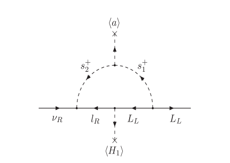
Figure 1: Induced Dirac neutrino mass

$$(M_{\nu})_{\alpha i}=-\frac{\mu f_{a}}{8\pi^{2}m_{\beta}}f_{\alpha\beta}h_{\beta i}I(m_{s1}^{2},m_{s2}^{2},m_{\beta}^{2})\,,$$ (3)

where $I(m_{s1}^{2},m_{s2}^{2},m_{\beta}^{2})$ is defined as

$$I(m_{s1}^{2},m_{s2}^{2},m_{\beta}^{2})=\frac{m_{\beta}^{2}}{m_{s1}^{2}-m_{s2}^{2}}[\frac{m_{s1}^{2}}{m_{s1}^{2}-m_{\beta}^{2}}\log\frac{m_{s1}^{2}}{m_{\beta}^{2}}-\frac{m_{s2}^{2}}{m_{s2}^{2}-m_{\beta}^{2}}\log\frac{m_{s2}^{2}}{m_{\beta}^{2}}]\;.$$ (4)

In the limit of $m_{s1,2}\gg m_{k}$, the neutrino mass matrix is proportional to charged lepton mass, as given by

$$\begin{split}(M_{\nu})_{\alpha i}&=-\frac{1}{8\pi^{2}}f_{\alpha\beta}h_{\beta i}m_{\beta}\frac{\mu f_{a}}{m_{s1}^{2}-m_{s2}^{2}}\log\frac{m_{s1}^{2}}{m_{s2}^{2}}\\ &\approx-\frac{1}{8\pi^{2}}f_{\alpha\beta}h_{\beta i}{\mu m_{\beta}\over m_{a}}\frac{\Lambda_{\mathrm{QCD}}^{2}}{m_{s1}^{2}-m_{s2}^{2}}\log\frac{m_{s1}^{2}}{m_{s2}^{2}}=-Cf_{\alpha\beta}m_{\beta}h_{\beta i}.\end{split}$$ (5)

We have replaced the PQ-symmetry breaking scale by the axion mass and the QCD scale in Eq. (5) . Note that there are similar construction discussed in Refs. Nasri:2001ax ; Kanemura:2011jj . However, our setup shows the interesting relation between the neutrino Dirac mass and QCD dynamics. Furthermore, the axions can be the dark matter candidate constituting of $25\%$ of energy density in our universe. From the neutrino mass formula and scalar potential we can see that if one does not tune the couplings $h_{a1}$ and $h_{a2}$, then the masses of $s_{1}$ and $s_{2}$ should be of the order of $f_{a}$. Combining with the value of $\mu$ to be around the electroweak scale would directly lead to a small quantity of $C\approx 10^{-8}$, which means one can have the observed light neutrino masses with the Yukawa couplings $f,h$ at the order of $10^{-1}$. Although such a scenario can naturally provide a tiny neutrino mass without fine tuning the couplings, in what follows we still focus on the case in which both $m_{s1}$ and $m_{s2}$ are of the electroweak scale to provide richer phenomenological implications. In this case we can see that the large value of $f_{a}$ lifts up the mass scale of Dirac neutrino masses and in order to keep the smallness of $M_{\nu}$ a combination of suppressed factors will be needed such as the loop factor, the Yukawa couplings $f$, $h$, the charged lepton chirality suppression, and the parameter $\mu$. Now we roughly estimate the scale of $\mu$ which is the key parameter controlling the overall mass scale of Dirac neutrino masses and a investigation of parameter space will be discussed in section III. For $M_{\nu}\approx 0.1$ eV, $m_{s_{1,2}}\sim\mathcal{O}(100-1000)$ GeV, and $f_{a}\approx 10^{12}$ GeV, we have $f\sim 10^{-3}$, $h\sim 10^{-2}$, and $\mu\sim\mathcal{O}(1)$ keV. Let’s make two comments on the low scale $\mu$ and Dirac neutrino masses : 1. We can explain the small $\mu$ by implementing the Froggatt-Nielsen mechanism CERN-TH-2519 with PQ-symmetry. For example, if we assign the PQ quantum number of $a$ as $\frac{2}{n}$ in Table 1, all the terms in the Lagrangian will not change except the $\mu$-coupling in the potential. One can write the effective operator as

$$\frac{1}{\Lambda^{n-2}}s_{1}^{+}s_{2}^{-}a^{n}\xrightarrow[U(1)_{PQ}~{}breaking]{}(\frac{\langle a\rangle}{f_{a}})^{n-2}\langle a\rangle s_{1}^{+}s_{2}^{-}a,$$ (6)

thus $\mu=(\frac{\langle a\rangle}{f_{a}})^{n-2}\langle a\rangle$ at low energy scale and can be tuned to a small quantity. Here the PQ symmetry can be broken dynamically by some condensates of a new technicolor-like interaction at high scale Kim:1984pt ; Choi:1985cb . This mechanism can also apply to other dimensionless couplings of non-Hermitian terms such as the $h_{5}$ in the potential. 2. The mass scale of Dirac neutrino masses is not necessarily small if neutrinos are Majorana fermions. Although we consider neutrinos as the Dirac fermions, the main concern in this paper is the origin of the Dirac neutrino mass, which in general does not forbidden the possibility that neutrinos are the Majorana fermions. Therefore one can still have heavy right-handed Majorana masses as inspired by the grand unification theories and obtain small neutrino masses through canonical seesaw mechanism. The goal in this paper is to point out that the Dirac neutrino mass is generated by the PQ-symmetry breaking.

III Confronting with neutrino oscillation data and leptonic rare decays

From the standard formalism $M_{\nu}$ can be diagonalized by

$$M_{\nu_{diag}}=V_{\mathrm{PMNS}}^{\dagger}M_{\nu}V_{R}^{\nu\dagger}=-V_{\mathrm{PMNS}}^{\dagger}(CfM_{l_{diag}}h)V_{R}^{\nu\dagger},$$ (7)

where $V_{\rm PMNS}$ is a unitary $3\times 3$ Pontecorvo-Maki-Nakagava-Sakata (PMNS) matrix and $V_{R}$ is the transformation matrix for right-handed neutrinos. For convenience we define $FH=V_{\mathrm{PMNS}}M_{\nu_{diag}}$ with $H=M_{l_{diag}}(-hV_{R}^{\nu\dagger})$ and $F=Cf$. Due to the anti-symmetric nature of $f$ matrix, the lightest neutrino is exactly massless in this model. Therefore, we can multiply a transformation matrix $A$ to both sides of the mass matrix to reduce one row in the left hand side of Eq. (7). One obtain

$$F^{\prime}H=AV_{\mathrm{PMNS}}M_{\nu_{diag}},$$ (8)

where

$$F^{\prime}=AF=\left(\begin{array}[]{ccc}-F_{e\mu}&0&F_{\mu\tau}\\ F_{e\tau}&F_{\mu\tau}&0\\ 0&0&0\\ \end{array}\right),A=\left(\begin{array}[]{ccc}0&1&0\\ 0&0&-1\\ F_{\mu\tau}&-F_{e\tau}&F_{e\mu}\\ \end{array}\right).$$ (9)

Then we have

$$\begin{split}&\left(\begin{array}[]{ccc}-F_{e\mu}H_{e1}+F_{\mu\tau}H_{\tau 1}&-F_{e\mu}H_{e2}+F_{\mu\tau}H_{\tau 2}&-F_{e\mu}H_{e3}+F_{\mu\tau}H_{\tau 3}\\ F_{e\tau}H_{e1}+F_{\mu\tau}H_{\mu 1}&F_{e\tau}H_{e2}+F_{\mu\tau}H_{\mu 2}&F_{e\tau}H_{e3}+F_{\mu\tau}H_{\mu 3}\\ 0&0&0\\ \end{array}\right)\\ &=\left(\begin{array}[]{ccc}m_{\nu 1}V_{\mu 1}&m_{\nu 2}V_{\mu 2}&m_{\nu 3}V_{\mu 3}\\ -m_{\nu 1}V_{\tau 1}&-m_{\nu 2}V_{\tau 2}&-m_{\nu 3}V_{\tau 3}\\ m_{\nu 1}\sum_{l}V_{l1}F_{l}&m_{\nu 2}\sum_{l}V_{l2}F_{l}&m_{\nu 3}\sum_{l}V_{l3}F_{l}\\ \end{array}\right)\end{split}$$ (10)

with $F_{l}=(F_{\mu\tau},-F_{e\tau},F_{e\mu})$.

For the normal hierarchical spectrum with $m_{\nu_{1}}=0$ we have the following relations :

$$F_{e\mu}={V_{\tau 1}^{*}\over V_{e1}^{*}}F_{\mu\tau}\,,\,F_{e\tau}=-{V_{\mu 1}^{*}\over V_{e1}^{*}}F_{\mu\tau}\,,$$ (11)

and

$$H_{\mu 1}={V_{\mu 1}^{*}\over V_{e1}^{*}}H_{e1}\,,\,H_{\tau 1}={V_{\tau 1}^{*}\over V_{e1}^{*}}H_{e1}.$$ (12)

The other terms give $H_{\mu 2}$, $H_{\mu 3}$, $H_{\tau 2}$, $H_{\tau 3}$ in terms of $F_{\mu\tau}$, $H_{e2}$ and $H_{e3}$

$$\begin{split}H_{\mu 2}&={V_{\mu 1}^{*}\over V_{e1}^{*}}H_{e2}-{m_{\nu_{2}}\over F_{\mu\tau}}V_{\tau 2}\;,\;H_{\tau 2}={V_{\tau 1}^{*}\over V_{e1}^{*}}H_{e2}+{m_{\nu_{2}}\over F_{\mu\tau}}V_{\mu 2}\,,\,\\ H_{\mu 3}&={V_{\mu 1}^{*}\over V_{e1}^{*}}H_{e3}-{m_{\nu_{3}}\over F_{\mu\tau}}V_{\tau 3}\;,\;H_{\tau 3}={V_{\tau 1}^{*}\over V_{e1}^{*}}H_{e3}+{m_{\nu_{3}}\over F_{\mu\tau}}V_{\mu 3}\,.\end{split}$$ (13)

Note that the requirement of real $F$ matrix make $V_{\mathrm{PMNS}}$ include two addition phases besides the ordinary irreducible one. Therefore, the model will not give a conclusive prediction for the Dirac CP phase in the neutrino sector at current stage.

Similarly for the inverted hierarchical spectrum, $m_{\nu_{3}}=0$, we obtain

$$\begin{split}F_{e\mu}&={V_{\tau 3}^{*}\over V_{e3}^{*}}F_{\mu\tau}\,,\,F_{e\tau}=-{V_{\mu 3}^{*}\over V_{e3}^{*}}F_{\mu\tau}\,,\\ H_{\mu 1}&={V_{\mu 3}^{*}\over V_{e3}^{*}}H_{e1}-{m_{\nu_{1}}\over F_{\mu\tau}}V_{\tau 1}\,,\,H_{\tau 1}={V_{\tau 3}^{*}\over V_{e3}^{*}}H_{e1}+{m_{\nu_{1}}\over F_{\mu\tau}}V_{\mu 1},\\ H_{\mu 2}&={V_{\mu 3}^{*}\over V_{e3}^{*}}H_{e2}-{m_{\nu_{2}}\over F_{\mu\tau}}V_{\tau 2}\;,\;H_{\tau 2}={V_{\mu 3}^{*}\over V_{e3}^{*}}H_{e2}+{m_{\nu_{2}}\over F_{\mu\tau}}V_{\mu 2}\,,\,\\ H_{\mu 3}&={V_{\mu 3}^{*}\over V_{e3}^{*}}H_{e3}\;,\;H_{\tau 3}={V_{\tau 3}^{*}\over V_{e3}^{*}}H_{e3}\,.\end{split}$$ (14)

$\sin^{2}\theta_{12}$	$\sin^{2}\theta_{23}$	$\sin^{2}\theta_{13}$	$\Delta m_{sun}^{2}$	$\Delta m_{atm}^{2}$
$0.30\pm 0.013$	$0.41^{+0.037}_{-0.025}$	$0.023\pm 0.0023$	$(7.50\pm 0.185)\times 10^{-5}\mathrm{eV}^{2}$	$(2.47^{+0.069}_{-0.067})\times 10^{-3}\mathrm{eV}^{2}$

Table 2: Neutrino oscillation data.

We will use the central values of the most recently global fitting of the neutrino oscillation measurements GonzalezGarcia:2012sz (see Table 2) in our analyses. In the meantime the appearance of the new scalars will provide the extra contributions to the lepton flavor violation processes. We investigate the parameter space of the model in terms of the constraints from leptonic rare decays in the following. Before that it is worth mentioning that the size of parameter $C$ is proportional to the factor $\mu f_{a}/(m_{s1}^{2}-m_{s2}^{2})\log(m_{s1}^{2}/m_{s2}^{2})$. If there exists a large hierarchy between $m_{s1}$ and $m_{s2}$, say, $m_{s2}=km_{s1}$ with $k$ being a large factor, $C$ is approximately inverse proportional to $m_{s2}^{2}$. However, the positive mass eigenvalue condition $m_{s1}m_{s2}>\mu f_{a}$ will also lead to the result that the upper bound of $C$ is proportional to $1/k$. In general $C$ can not be too small in order to keep the perturbativity of the Yukawa coupling $f$ and $h$. So the largest allowed hierarchy between $m_{s1}^{2}$ and $m_{s2}^{2}$ is around $k\simeq O(10^{3})$. We will also discuss the implication to the parameter space with a hierarchy scenario.

III.1 $\mu\to e\gamma$

The two relevant Yukawa interactions providing the flavor violations in charged lepton sector are given by

$$\mathcal{L}=-2f_{\alpha\beta}\overline{l_{L_{\alpha}}^{c}}\nu_{L_{\beta}}s_{1}-h_{\alpha i}\overline{l_{R_{\alpha}}^{c}}\nu_{R_{i}}s_{2}+\mathrm{h.c.}.$$ (15)

Without loss of generality here $\nu_{R_{i}}$ is the mass eigenstate and we absorb the mixing matrix $-V_{R}$ into the coupling $h$. In $\mathrm{SM}+\nu_{R}$ the one-loop contribution is constrained stringently by the Glashow-Iliopoulos-Maiani (GIM) mechanism. In this model the main contribution is the one-loop diagrams with photon emission attached to the charged scalars $s_{1}^{+}$ or $s_{2}^{+}$ in the loop. Currently the latest result from MEG collaboration gives $B(\mu\rightarrow e\gamma)<2.4\times 10^{-12}$ Adam:2011ch . For $l_{\alpha}\to l_{\beta}\gamma$ the effective Lagrangian can be generally written in the form

$$\mathcal{L}=-{1\over 2}\bar{l}_{\beta}\sigma_{\mu\nu}(\tilde{A}_{R}P_{R}+\tilde{A}_{L}P_{L})l_{\alpha}F^{\mu\nu},$$ (16)

where $\tilde{A}_{L,R}$ for this model is given by

$$\tilde{A}_{R}=\frac{(-1)e}{192\pi^{2}}(4\sum_{\gamma}f_{\beta\gamma}^{*}f_{\alpha\gamma}){m_{\alpha}\over m_{s1}^{2}}\quad{\rm and}\quad\tilde{A}_{L}=\frac{(-1)e}{192\pi^{2}}(\sum_{i}h_{\beta i}^{*}h_{\alpha i}){m_{\alpha}\over m_{s2}^{2}}\,.$$ (17)

Note that the limit $m_{\alpha}\ll m_{s1,2}$ have been applied to the above formula. The decay rate of $l_{\alpha}\to l_{\beta}\gamma$ is $\Gamma(l_{\alpha}\to l_{\beta}\gamma)=(m_{\alpha}^{3}/16\pi)(1-m_{\beta}^{2}/m_{\alpha}^{2})^{3}(|\tilde{A}_{R}|^{2}+|\tilde{A}_{L}|^{2})$. One can compare it with the lepton three body decay width $\Gamma(l_{\alpha}\rightarrow l_{\beta}\nu_{\alpha}\bar{\nu}_{\beta})=G_{F}^{2}m_{\alpha}^{5}/192\pi^{3}$. The branching ratio $\mu\rightarrow e\gamma$ in our model is obtained by

$$\text{B}(\mu\to e\gamma)\equiv\frac{\Gamma(\mu\to e\gamma)}{\Gamma(\mu\rightarrow e\nu\bar{\nu})}=\frac{\alpha_{e}}{768\pi G_{F}^{2}}\bigg{(}{16\sum_{\gamma}|f_{e\gamma}|^{2}|f_{\mu\gamma}|^{2}\over m_{s1}^{4}}+{\sum_{i}|h_{ei}|^{2}|h_{\mu i}|^{2}\over m_{s2}^{4}}\bigg{)}\;.$$ (18)

The results are given in Fig. 2. Here we consider that $f_{\mu\tau}$ is positive for the normal hierarchy spectrum and negative for the inverted hierarchy spectrum, respectively. The allowed regions are rather small and sensitive to the value of $C$. For example, the parameter space will shrink to zero if we take $C=0.8\times 10^{-5}$ with the same inputs.

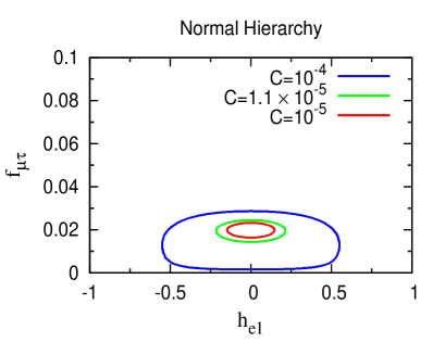
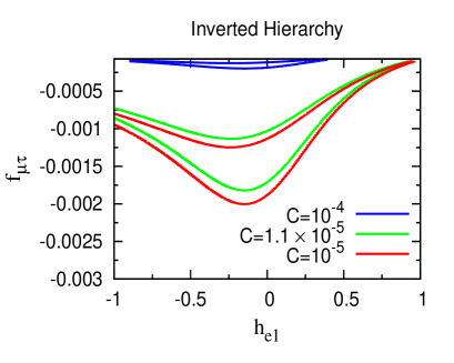
Figure 2: The allowed region in $h_{e1}-f_{\mu\tau}$ plane in (a) the normal hierarchy, and (b) the inverted hierarchy. Different curves are generated with different $C$ (blue: $C=10^{-4}$, green: $C=1.1\times 10^{-5}$, red: $C=10^{-5}$). The other parameters are taken as $m_{s1}=m_{s2}=500\mathrm{GeV}$, $h_{e2}=h_{e3}=0.5$.

III.2 $\mu-e$ conversion

The one loop diagrams to $\mu-e$ conversion include photon penguin diagrams, Z penguin diagrams, and box diagrams. Again the contribution from the diagrams involving W boson exchange is suppressed by GIM mechanism and the leading contributions come from the penguin diagrams with the charged scalars $s_{1}^{+}$ and $s_{2}^{+}$ in the loop. In contrast, the leading Z penguin contribution is suppressed by the light charged scalars. Therefore only photon penguin needs to be taken into account. The corresponding effective Lagrangian is given by

$$\mathcal{L}=-\frac{G_{F}}{\sqrt{2}}\frac{s_{W}^{2}}{36\pi^{2}}m_{W}^{2}\bar{e}\gamma_{\mu}(\sum_{\alpha}4f_{e\alpha}^{*}f_{\mu\alpha}\frac{1}{m_{s1}^{2}}P_{L}+\sum_{i}h_{ei}^{*}h_{\mu i}\frac{1}{m_{s2}^{2}}P_{R})\mu\sum_{q}Q_{q}\bar{q}\gamma^{\mu}q\,.$$ (19)

In the above we used the shorthand notation $s_{W}\equiv\sin{\theta_{W}}$. The $\mu-e$ conversion with nucleon in atom has been calculated in details in Ref. Kitano:2002mt , and we will adopt their notation in what follows. The general interactions associated with $\mu-e$ conversion are written as

$$\begin{split}\mathcal{L}_{\mathrm{eff}}&=-{4G_{F}e\over\sqrt{2}}[m_{\mu}\bar{e}\sigma^{\mu\nu}(A_{R}P_{R}+A_{L}P_{L})\mu F_{\mu\nu}+\mathrm{h.c.}]\\ &-{G_{F}\over\sqrt{2}}[\bar{e}(g_{LS(q)}P_{R}+g_{RS(q)}P_{L})\mu\bar{q}q+\bar{e}(g_{LP(q)}P_{R}+g_{RP(q)}P_{L})\mu\bar{q}\gamma_{5}q+\mathrm{h.c.}]\\ &-{G_{F}\over\sqrt{2}}[\bar{e}(g_{LV(q)}\gamma^{\mu}P_{L}+g_{RV(q)}\gamma^{\mu}P_{R})\mu\bar{q}\gamma_{\mu}q+\bar{e}(g_{LA(q)}\gamma^{\mu}P_{L}+g_{RA(q)}\gamma^{\mu}P_{R})\mu\bar{q}\gamma_{\mu}\gamma_{5}q+\mathrm{h.c.}]\\ &-{G_{F}\over\sqrt{2}}\bigg{[}{1\over 2}\bar{e}(g_{LT(q)}\sigma^{\mu\nu}P_{R}+g_{RT(q)}\sigma^{\mu\nu}P_{L})\mu\bar{q}\sigma_{\mu\nu}q+\mathrm{h.c.}\bigg{]}\,,\end{split}$$ (20)

where $A_{R,L}$ is related to the dipole interaction with photon, and $g_{S,P,V,A,T}$ indicate scalar, pseudoscalar, vector, axial vector and tensor couplings, respectively. Comparing the above formula with Eq. (19), we have

$$g_{LV}^{(q)} =\frac{Q_{q}s_{W}^{2}}{36\pi^{2}}m_{W}^{2}(\sum_{\alpha}4f_{e\alpha}^{*}f_{\mu\alpha}\frac{1}{m_{s1}^{2}})\,,\,g_{RV}^{(q)}=\frac{Q_{q}s_{W}^{2}}{36\pi^{2}}m_{W}^{2}(\sum_{i}h_{ei}^{*}h_{\mu i}\frac{1}{m_{s2}^{2}})\;,$$ (21a)

$$A_{R} =\frac{(-1)}{192\pi^{2}g_{2}^{2}}(\sum_{\alpha}4f_{e\alpha}^{*}f_{\mu\alpha}{m_{W}^{2}\over m_{s1}^{2}})\;,A_{L}=\frac{(-1)}{192\pi^{2}g_{2}^{2}}(\sum_{i}h_{ei}^{*}h_{\mu i}{m_{W}^{2}\over m_{s2}^{2}}),$$ (21b)

and other couplings vanish. The rate of $\mu-e$ conversion with nucleons in atom $A$ is usually normalized to the rate of muon capture by $A$. The conversion-to-capture ratio can be derived in the form

$$B_{\mu\rightarrow e}^{A}={2G_{F}^{2}m_{\mu}^{5}\over\Gamma_{\mathrm{capt}}^{A}}(|eA_{R}D+\tilde{g}_{LV}^{(p)}V^{(p)}+\tilde{g}_{LV}^{(n)}V^{(n)}|^{2}+|eA_{L}D+\tilde{g}_{RV}^{(p)}V^{(p)}+\tilde{g}_{RV}^{(n)}V^{(n)}|^{2})\;$$ (22)

with $\tilde{g}_{L,RV}^{(p)}=2g_{L,RV}^{(u)}+g_{L,RV}^{(d)}$ and $\tilde{g}_{L,RV}^{(n)}=g_{L,RV}^{(u)}+2g_{L,RV}^{(d)}$. $D$ and $V^{(p,n)}$ are overlapped functions which can be found in Ref. Kitano:2002mt . The constraints from experimental results for $\mu-e$ conversion in different nuclei Bertl:2006up ; Badertscher:sulfer ; Badertscher:1981ay ; Dohmen:1993mp ; Honecker:1996zf are weaker than what’s given by $\mu\rightarrow e\gamma$.

III.3 $\mu\rightarrow 3e$

Penguin diagrams and Box diagrams contribute to this process. The experimental upper bounds is $B(\mu\rightarrow e\bar{e}e)<10^{-12}$ Bellgardt:1987du . SM with right-handed neutrino singlets contribution to this processes is suppressed by the neutrino mass. The corresponding one loop diagrams in this model for $\mu\rightarrow 3e$ are similar to those for $\mu-e$ conversion, with the quarks replaced by electrons. In general the effective Lagrangian for $\mu\rightarrow e\bar{e}e$ is

$$\begin{split}\mathcal{L}(\mu\rightarrow e\bar{e}e)&=-{4G_{F}\over\sqrt{2}}[\bar{e}\gamma_{\mu}e{q_{\nu}\over q^{2}}\bar{e}i\sigma^{\mu\nu}(8\pi\alpha_{e}m_{\mu})(A_{R}P_{R}+A_{L}P_{L})\mu\\ &+\bar{e}\gamma^{\mu}(a_{L}P_{L}+a_{R}P_{R})e\bar{e}\gamma_{\mu}P_{L}\mu+\bar{e}\gamma^{\mu}(b_{L}P_{L}+b_{R}P_{R})e\bar{e}\gamma_{\mu}P_{R}\mu]\,.\end{split}$$ (23)

The branching ratio can be calculated as

$$\begin{split}B(\mu\rightarrow e\bar{e}e)&\simeq(|a_{R}|^{2}+|b_{L}|^{2})+2(|a_{L}|^{2}+|b_{R}|^{2})-32\pi\alpha_{e}\mathrm{Re}(A_{R}(a_{R}+2a_{L})+A_{L}(b_{L}+2b_{R}))\\ &+256\pi^{2}\alpha_{e}^{2}(|A_{R}|^{2}+|A_{L}|^{2})\bigg{(}4\ln{m_{\mu}\over m_{e}}-{11\over 2}\bigg{)}\,,\end{split}$$ (24)

where the parameters $a_{L,R}$ and $b_{L,R}$ are given by

$$a_{L,R}=-\frac{s_{W}^{2}}{144\pi^{2}}m_{W}^{2}(\sum_{\alpha}4f_{e\alpha}^{*}f_{\mu\alpha}\frac{1}{m_{s1}^{2}})\quad{\rm and}\quad b_{L,R}=-\frac{s_{W}^{2}}{144\pi^{2}}m_{W}^{2}(\sum_{i}h_{ei}^{*}h_{\mu i}\frac{1}{m_{s2}^{2}})\,$$ (25)

from the photon penguin diagrams, while for the box diagrams the leading order of $a^{\rm box}_{R}$ and $b^{\rm box}_{L}$ vanishing, we have

$$a^{\rm box}_{L}={m_{W}^{2}\over 32\pi^{2}g_{2}^{2}m_{s1}^{2}}|\sum_{\alpha}4f_{\mu\alpha}f_{e\alpha}^{*}||\sum_{\alpha^{\prime}}4f_{e\alpha^{\prime}}^{*}f_{e\alpha^{\prime}}|$$ (26a)

and

$$b^{\rm box}_{R}={m_{W}^{2}\over 32\pi^{2}g_{2}^{2}m_{s2}^{2}}|\sum_{i}h_{\mu i}h_{ei}^{*}||\sum_{i^{\prime}}h_{ei^{\prime}}^{*}h_{ei^{\prime}}|$$ (26b)

respectively. As shown in Fig. 2 the Yukawa coupling $f$ is in the range of $\cal{O}$($10^{-2}$) to $\cal{O}$($10^{-3}$); we can safely ignore the box diagram contributions in $\mu\rightarrow 3e$ decay. Therefore, the parameter space is looser to those of $\mu\rightarrow e\gamma$.

In the limit of mass hierarchy between $m_{s1}$ and $m_{s2}$, that is, $m_{s1}>m_{s2}$ or $m_{s2}>m_{s1}$ cases, the parameter space for Yukawa couplings $h$ and $f$ in both normal hierarchy and inverted hierarchy neutrino mass spectrum respectively are shown in Fig. 3 and Fig. 4. Here we take $m_{s1}=20m_{s2}$ and $m_{s2}=5m_{s1}$ as the reference points. In these cases, we are only able to give a severe constraint on one of the couplings, $h$ or $f$, and we illustrate our results by taking $500$ GeV mass scale to the lighter scalar field.

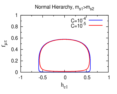
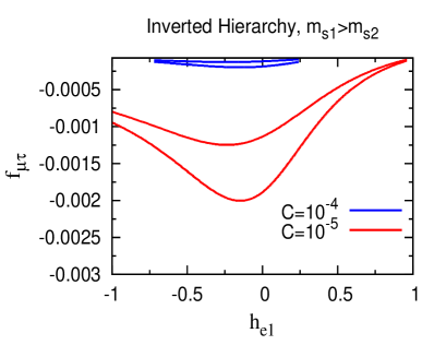
Figure 3: The allowed region in $h_{e1}-f_{\mu\tau}$ plane for the case of $m_{s1}=20m_{s2}$ in normal hierarchy and inverted hierarchy neutrino mass spectrum respectively. Blue line corresponds to $C=10^{-4}$ and Red line represents $C=10^{-5}$.

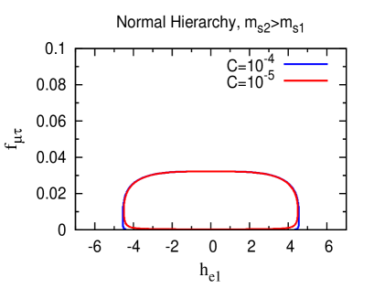
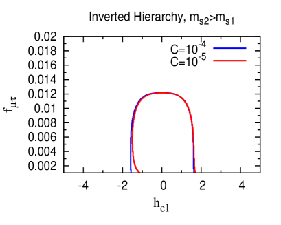
Figure 4: The allowed region in $h_{e1}-f_{\mu\tau}$ plane for the case of $m_{s2}=5m_{s1}$ in normal hierarchy and inverted hierarchy neutrino mass spectrum respectively. Blue line corresponds to $C=10^{-4}$ and Red line represents $C=10^{-5}$.

IV Phenomenology

IV.1 electromagnetic moments of leptons

IV.1.1 muon $g-2$

The anomalous magnetic moment of the muon is an observable as a precision test to the SM. The current experimental results Bennett:2006fi ; pdg2012 reported that the muon $g-2$ deviation from the SM prediction is $a_{\mu}(\rm{exp})-a_{\mu}(\rm{SM})=(287\pm 63\pm 49)\times 10^{-11}$, which indicates some new physics contribution. Since our scenario is essentially a two Higgs doublet model (2HDM) plus two singly charged scalars $s^{\pm}_{1}$ and $s^{\pm}_{2}$. The anomalous $g-2$ of muon in this model is given by

$$\begin{split}\Delta a_{\mu}=-{m_{\mu}^{2}\over 96\pi^{2}}&[4\sum_{\alpha}|f_{\mu\alpha}|^{2}\frac{1}{m_{s1}^{2}}+\sum_{i}|h_{\mu i}|^{2}\frac{1}{m_{s2}^{2}}\\ &+{m_{\mu}^{2}\over v^{2}}({14c_{\beta-\alpha}^{2}\over m_{h}^{2}\cos^{2}\beta}+{14s_{\beta-\alpha}^{2}\over m_{H}^{2}\cos^{2}\beta}-{22\tan^{2}\beta\over m_{A}^{2}}+{\tan^{2}\beta\over m_{H^{+}}^{2}})]\;,\end{split}$$ (27)

where $h$ and $H$ are scalar particles with $h$ being the SM-like Higgs, as well as the pseudo-scalar field $A$ and the charged scalars $H^{\pm}$. $\alpha$, $\beta$ are the mixing angles ($s_{\beta-\alpha}\equiv\sin{(\beta-\alpha)}$ and $c_{\beta-\alpha}\equiv\cos{(\beta-\alpha)}$) defined in the usual 2HDM (see e.g. Branco:2011iw ; Chang:2012ta and references within). Comparing with the current experimental result, our model gives a rather small contribution to $\Delta{a_{\mu}}$ but still within the experimental errors.

IV.1.2 magnetic moments of neutrinos

Neutrinos can have magnetic moment when they are massive. The present upper bound of neutrino magnetic moment from experiments is $\mu_{\nu}<3.2\times 10^{-11}\mu_{B}$ Beda:2009kx . The ordinary leading order contribution in SM including right-handed Dirac neutrino is the exchange of $W$, which is around $(3.2\times 10^{-19}\mu_{B})(m_{\nu_{i}}/\mathrm{eV})$ Fujikawa:1980yx with the Bohr magneton $\mu_{B}\equiv e/2m_{e}$. In this model, the main new contribution comes from the mixing of $s^{+}_{1,2}$ in the loop since the same diagram also generates neutrino masses, given by

$$|\mu_{\nu}^{s}|=2m_{i}e(\log{m_{s2}^{2}\over m_{s1}^{2}})^{-1}({1\over m_{s1}^{2}}-{1\over m_{s2}^{2}})\approx 10^{-19}\mu_{B}.$$ (28)

Note that it only depends on the neutrino and scalar masses, and this contribution is comparable with that associated with W exchange. It is understandable that without imposing a symmetry Voloshin:1987qy or employing a spin suppression mechanism to $m_{\nu}$ Barr:1990um , the generic size of the Dirac neutrino magnetic moment can not excess $10^{-14}\mu_{B}$ Bell:2005kz . The contributions from other charged scalars such as $H^{+}$, $s^{+}_{1}$, and $s_{2}^{+}$ in the loop are less than $\mathcal{O}(10^{-25})\mu_{B}$ as a result that they do not contribute to neutrino masses.

IV.1.3 EDM of leptons

Since there is a physical CP phase among the Yukawa couplings $f$ and $h$, in general, we have the new contributions to the electric dipole moment of charged leptons. The exchange of singly charged scalars gives the EDM to the charged leptons at one-loop level as

$$d_{l}=-\frac{e}{(4\pi)^{2}}\sum_{i}\mathrm{Im}(2h_{li}^{*}(fV)_{li})\frac{\mu f_{a}}{m_{s1}^{2}-m_{s2}^{2}}[{1\over m_{s1}}B\left(\frac{m_{\nu_{i}}^{2}}{m_{s1}^{2}}\right)-{1\over m_{s2}}B\left(\frac{m_{\nu_{i}}^{2}}{m_{s2}^{2}}\right)]\;,$$ (29)

with the function $B(x)$ defined by

$$B(x)=\frac{\sqrt{x}}{2(1-x)^{2}}\left(1+x+\frac{2x\ln(x)}{1-x}\right).$$ (30)

Therefore we conclude that the extra contribution is smaller than $\mathcal{O}({m_{\nu}^{2}\over m_{l}m_{s}^{2}})$, which means $|d_{e}|\lesssim 10^{-35}e\,\mathrm{cm}$. Similarly, the neutrino EDM generated by $s^{+}_{1,2}$ mixing in the loop gives $|d_{\nu}|\lesssim 10^{-26}e\,\mathrm{cm}$. Though the new contributions to $d_{e}$ and $d_{\nu}$ are nonzero, both of them are unobservably small.

IV.2 dark matter

It is known that the axion field can be a dark matter candidate constituting a significant fraction of energy density in our universe. For the purpose of completion we briefly review some aspects of this scenario in this subsection. The properties of the invisible axion are determined by the breaking scale $f_{a}$ where its mass and the interactions are inverse proportional to $f_{a}$. Hence the invisible axion is a very light, very weakly interacted and very long-lived particle. Axions with mass in the range of $10^{-5}-10^{-6}$ eV were produced during the QCD phase transition with the average momentum of order the Hubble expansion rate ($\sim 3\times 10^{-9}$ eV) at this epoch and hence are cold dark matter (CDM). Their number density is provided by

$$\Omega_{a}\simeq\frac{1}{2}(\frac{0.6\times 10^{-5}~{}\rm{eV}}{m_{a}})^{\frac{7}{6}}(\frac{0.7}{h})^{2},$$ (31)

where $h$ is the current Hubble expansion rate in units of 100$\rm{kms^{-1}Mpc^{-1}}$. Here we assume the ratio of the axion number density to the entropy density is constant since produced and the contribution from topological defects decay is negligible. Recently it was pointed out that the CDM axions would form a Bose-Einstein condensate due to their gravitational interactions Sikivie:2009qn . Furthermore the rethermalization process is so fast that the lowest energy state of the degenerate axion gas consists of a nonzero angular momentum. As a result a ”caustic ring” structure may form in the inner galactic halo Erken:2011dz ; Sikivie:1997ng ; Sikivie:1999jv . The feature would make the axion a different dark matter from other CDM candidates, and we refer readers to the references Sikivie:2009qn ; Erken:2011dz ; Sikivie:1997ng ; Sikivie:1999jv for details.

IV.3 $h\rightarrow\gamma\gamma$

We closing our discussion on phenomenology with investigating the LHC Higgs results. Both ATLAS :2012gk and CMS :2012gu have announced the discovery of a new boson at a mass of 125 GeV which is consistent with the SM Higgs boson via the combined analyses of the $\gamma\gamma$ and $ZZ$ channels. However, the precise values of both production cross sections and decay branch ratios of the new resonance need to be measured to compare with those predictions from the SM. It was pointed out that the branching ratio of Higgs decay into two photons has excess about $1.56\pm 0.43$ and $1.9\pm 0.5$ times than the SM prediction in both CMS :2012gu and ATLAS :2012gk collaborations data in 2012. A updated results can be found in ATLAS_NOTE_2013_034 and moriond2 . Although the deviation is still within the SM expectations at $2\sigma$ level, one may consider whether there are new physics effects (see e.g. Cacciapaglia:2009ky ; Cao:2011pg ; Ellwanger:2011aa ; Barger:2012hv ; Azatov:2012bz ; Giardino:2012ww ; Carena:2012xa ; Christensen:2012ei ; Carena:2012gp ; Chang:2012ta ; Chiang:2012qz and references therein) In particular, new scalars particles have been widely treated as possible sources. We study the implications of Higgs to di-phonton and Higgs to Z-photon decay channels in our model. For simplicity we just consider one singly charged scalar $s^{\pm}$ and omit the subscript in this subsection. The SM Higgs production cross section is modified by the additional doublet scalar in our scenario Chang:2012ta ,

$$\sigma_{0}={G_{F}\alpha_{s}^{2}\over 128\sqrt{2}\pi}\bigg{|}{1\over 2}(s_{\alpha}+{c_{\alpha}\over\tan\beta})A_{1/2}(\tau_{t})+{1\over 2}(s_{\alpha}-c_{\alpha}\tan\beta)A_{1/2}(\tau_{b})\bigg{|}^{2}\;.$$ (32)

Notice that the bottom quark contribution is not negligible due the enhancement of large $\tan{\beta}$ and $A_{1/2}(\tau)=2[\tau+(\tau-1)f(\tau)]\tau^{-2}$ with $\tau_{i}=\frac{M^{2}_{h}}{4M^{2}_{i}}$. The function $f(\tau)$ is defined by

$$f(\tau)=\bigg{\{}\begin{array}[]{l}(\sin^{-1}\sqrt{\tau})^{2}\hskip 60.0pt,\tau\leq 1\\ -{1\over 4}[\log{1+\sqrt{1-\tau^{-1}}\over 1-\sqrt{1-\tau^{-1}}}-i\pi]^{2}\quad,\,\tau>1\,.\end{array}$$ (33)

In type-II 2HDM the decay rate of $h\rightarrow\gamma\gamma$ is given by

$$\begin{split}\Gamma_{\gamma\gamma}&={G_{F}\alpha^{2}m_{h}^{3}\over 128\sqrt{2}\pi^{3}}|(s_{\alpha}+{c_{\alpha}\over\tan\beta}){4\over 3}A_{1/2}(\tau_{t})+(s_{\alpha}-{c_{\alpha}\tan\beta}){1\over 3}A_{1/2}(\tau_{b})\\ &+s_{\alpha}A_{1}(\tau_{W})+\lambda^{\prime}A_{0}(\tau_{H^{+}})+\lambda A_{0}(\tau_{s^{+}})|^{2},\end{split}$$ (34)

where $A_{1}(\tau)=-[2\tau^{2}+3\tau+3(2\tau-1)f(\tau)]\tau^{-2}$, and $A_{0}(\tau)=-[\tau-f(\tau)]\tau^{-2}$. The coefficients $\lambda$ and $\lambda^{\prime}$ are defined as $\lambda={v\mu_{Hs^{+}s^{-}}/(2m_{s}^{2})}$ and $\lambda^{\prime}={v\mu_{HH^{+}H^{-}}/(2m_{H^{+}}^{2})}$, where $\mu_{Hs^{+}s^{-}}$ and $\mu_{HH^{+}H^{-}}$ are the related trilinear couplings in the Higgs potential. One can see that the effects of doublet scalar charged component $H^{+}$ and the singly charged singlet $s^{+}$ are indistinguishable. The reason is the lack of knowledge of scalar potential. For $h\rightarrow Z\gamma$ channel the decay width is written as Chen:2013vi

$$\begin{split}\Gamma_{Z\gamma}&={G_{F}^{2}m_{W}^{2}\alpha m_{h}^{3}\over 64\pi^{4}c_{W}^{2}}(1-m_{Z}^{2}/m_{H}^{2})^{3}\times\\ &\bigg{|}(s_{\alpha}+{c_{\alpha}\over\tan\beta}){({1\over 2}-{4\over 3}s_{W}^{2})}A_{1/2}(\eta_{t},\kappa_{t})+(s_{\alpha}-{c_{\alpha}\tan\beta}){({1\over 4}-{1\over 3}s_{W}^{2})}A_{1/2}(\eta_{b},\kappa_{b})\\ &+s_{\alpha}c_{W}^{2}A_{1}(\eta_{W},\kappa_{W})+({1\over 2}-s_{W}^{2})\lambda^{\prime}A_{0}(\eta_{H^{+}},\kappa_{H^{+}})+(-s_{W}^{2})\lambda A_{0}(\eta_{s^{+}},\kappa_{s^{+}})\bigg{|}^{2},\\ \end{split}$$ (35)

where $A_{1/2}(\eta,\kappa)=-4(I_{1}(\eta,\kappa)-I_{2}(\eta,\kappa))$, $A_{1}(\eta,\kappa)=-4(4-{4\over\kappa})I_{2}(\eta,\kappa)-[(1+{2\over\eta})({4\over\kappa}-1)-(5+{2\over\eta})]I_{1}(\eta,\kappa)$, and $A_{0}(\eta,\kappa)=2I_{1}(\eta,\kappa)$ with the parameters $\eta_{i}=\frac{4M^{2}_{i}}{M^{2}_{h}}$ and $\kappa_{i}=\frac{4M^{2}_{i}}{M^{2}_{Z}}$. Functions $I_{1}(\eta,\kappa)$ and $I_{2}(\eta,\kappa)$ are given as

$$I_{1}(\eta,\kappa)={\eta\kappa\over 2(\eta-\kappa)}+{\eta^{2}\kappa^{2}\over 2(\eta-\kappa)^{2}}[f(\eta^{-1})-f(\kappa^{-1})]+{\eta^{2}\kappa\over(\eta-\kappa)^{2}}[g(\eta^{-1})-g(\kappa^{-1})]$$ (36)

and

$$I_{2}(\eta,\kappa)=-{\eta\kappa\over 2(\eta-\kappa)}[f(\eta^{-1})-f(\kappa^{-1})]$$ (37)

with

$$g(x)=\bigg{\{}\begin{array}[]{ll}\sqrt{x^{-1}-1}(\sin^{-1}\sqrt{x})&,x\leq 1\\ {\sqrt{1-x^{-1}}\over 2}[\log{1+\sqrt{1-x^{-1}}\over 1-\sqrt{1-x^{-1}}}-i\pi]&,\,x>1\end{array}$$ (38)

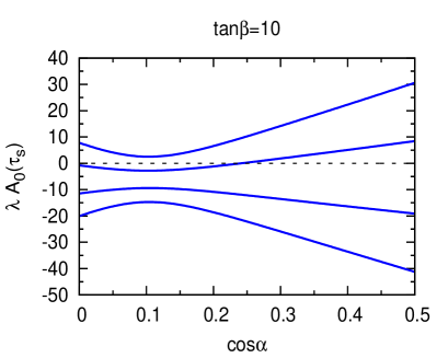
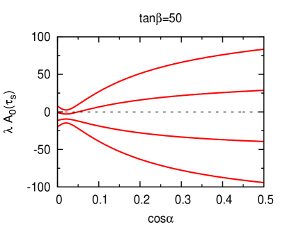
Figure 5: Solutions of $s^{+}$ effects in terms of $\cos{\alpha}$ by assuming $A_{0}(\eta,\kappa)/A_{0}(\tau)=1.00$ with $R_{\gamma\gamma}=\frac{\sigma_{\gamma\gamma}}{\sigma_{\gamma\gamma_{SM}}}=1.5$ and $R_{Z\gamma}=\frac{\sigma_{Z\gamma}}{\sigma_{Z\gamma_{SM}}}=1$. $\sigma_{ii}$ and $\sigma_{ii_{SM}}$ are the production cross sections for the Higgs to $ii$ channel in our model and SM respectively.

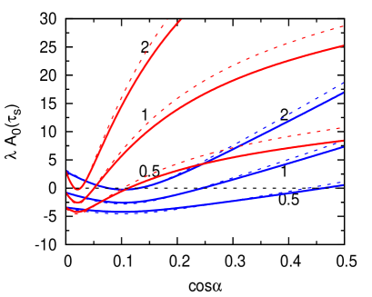
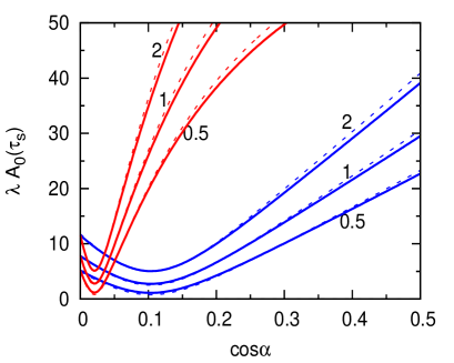
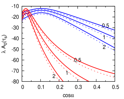
Figure 6: Effects of singly charged singlet scalar with values of $R_{Z\gamma}=0.5,1,2$ as indicated on each curves, and $A_{0}(\eta,\kappa)/A_{0}(\tau)=1.07$ (solid lines), $1.00$ (dashed lines) respectively for the fixed value $R_{\gamma\gamma}=1.5$. Blue lines correspond to $\tan{\beta}=10$ and Red lines represent $\tan{\beta}=50$. Note that each figure corresponds to one of the lines exhibited in Fig. 5.

respectively. Again we see from the Eq. (35) that the singly charged singlet effect is hidden in the 2HDM. In order to extract the information of $s^{+}$ from the decays we found the ratio of $A_{0}(\eta,\kappa)/A_{0}(\tau)$ lies in the range of $1.00-1.07$ with charged scalar masses above $100$ GeV. We then take the ratio as a constant and subtract the $H^{+}$ contributions in $\Gamma_{\gamma\gamma}$ and $\Gamma_{Z\gamma}$. Other SM Higgs decaying channels are calculated from HDECAY Djouadi:1997yw . The results of the $s^{+}$ effects in terms of the parameter $\cos{\alpha}$ with $\tan{\beta}=10$, $50$ are shown in Fig. 5. Here we take the values $R_{\gamma\gamma}=\frac{\sigma_{\gamma\gamma}}{\sigma_{\gamma\gamma_{SM}}}=1.5$ and $R_{Z\gamma}=\frac{\sigma_{Z\gamma}}{\sigma_{Z\gamma_{SM}}}=1$ with $\sigma_{ii}$ and $\sigma_{ii_{SM}}$ being the production cross sections for the Higgs to $ii$ channel in our model and SM respectively. Since the new physics effects can have both constructive and destructive interferences with the SM $W^{\pm}W^{\pm}$ amplitude, there are four lines exist in Fig. 5. The results of $s^{+}$ effects with different values of $R_{Z\gamma}$ and the ratio of $A_{0}(\eta,\kappa)/A_{0}(\tau)$ for the fixed $R_{\gamma\gamma}=1.5$ are shown in Fig. 6. Here $R_{Z\gamma}=0.5,1,2$ and $A_{0}(\eta,\kappa)/A_{0}(\tau)$ is taken to be $1.07$ and $1.00$ respectively. It shows that taking the ratio of $A_{0}(\eta,\kappa)/A_{0}(\tau)$ as a constant is a good approximation in the regions of parameters we are interested in and is useful for the deviation of $\Gamma_{Z\gamma}$ from the SM prediction for the singly charged singlet scalar $s^{+}$. Finally, it is worth to note that the charged singlet $s_{1}^{+}$ and $s_{2}^{+}$ can be produced by the quark annihilation through gauge boson $\gamma$ and $Z^{0}$ mediating. This process could have the final states including two charged leptons, the same as that of $pp\rightarrow h\rightarrow WW^{*}$, for which final states of $e$ or $\mu$ are tagged by LHC. The related signal strength observed from ATLAS is $1.3\pm 0.5$ ATLAS-conf-158 , and the $1\sigma$ deviation of it corresponds to around $20\mathrm{pb}$. This deviation can be regards as the allowed space for new contribution beyond SM. The singly charged scalar production cross section with parton distribution function given from CTEQ6 Pumplin:2002vw is also around $20\mathrm{pb}$ with $m_{s}\simeq 150\mathrm{GeV}$, which can be regarded as the lower bounds on $m_{s}$ if we assume $\mathrm{Br}(s\rightarrow e(\mu)\nu)\simeq 100\%$. Finally, we estimate the background contribution for $h\rightarrow WW^{*}\rightarrow e\nu\mu\nu$ channel from $s^{\pm}s^{\mp}$ production. Both singly charged scalars are off-shell and we found that the partial decay width for the center of mass in one of virtual scalar to be around $m_{W}$ is negligible compared to the SM prediction.

V Discussions and Conclusions

We investigate a model that neutrinos are Dirac fermions and their masses are generated from the Peccei-Quinn symmetry breaking at one-loop level. As a result the neutrino mass is related to $\Lambda_{\rm QCD}$ and axion is appeared to be a good candidate of dark matter in explaining the missing energy density of our universe. Leptonic rare decays constrain the model parameters severely, and therefore, the model can be tested in the near future. We also studied the implications of the new scalars to the electromagnetic moments of leptons and recent Higgs signals at LHC, specifically the $h\rightarrow\gamma\gamma$ and $h\rightarrow Z\gamma$ decays. Finally we would like to make a brief comment on the Majorana extension of our scenario. Lepton number symmetry is one of the key to understand the underlying neutrino physics. The smoking gun signals to resolve the question are $0\nu\beta\beta$ decays and some lepton number violating processes at LHC. Without the direct observations Majorana neutrinos and Dirac neutrinos are equally good in many aspects to describe the phenomena such as neutrino oscillations, leptogenesis, and Big Bang Nucleosynthesis, etc. Although we discuss the Dirac neutrino in this model and argue that the Dirac neutrino mass is originated from the Peccei-Quinn symmetry breaking which is well-motivated in QCD field theory, a Majorana masses of the right-handed neutrinos, in general, can be formed without violating any principle except the lepton number symmetry. The main modifications are to include some terms in the scalar potential such as $H_{1}H_{2}s_{1}^{+}$ and $H_{1}H_{2}as_{2}^{+}$. Therefore, our discussions can be easily embedded the scenario of Majorana neutrino and diagonalize the neutrino mass matrix via the seesaw mechanism.

Appendix A Scalar Mass Spectrum

We briefly analyze the scalar potential given in Eq. (2) and their particle spectrum in this appendix. If the neutral components of $H_{1}=(h_{1}^{+},\;(R_{1}+iA_{1})/\sqrt{2})^{T}$, $H_{2}=(h_{2}^{+},\;(R_{2}+iA_{2})/\sqrt{2})^{T}$ and $a=(R_{a}+iA_{a})/\sqrt{2}$ acquire the vacuum expectation values (VEVs) $v_{1}$, $v_{2}$, and $v_{a}$, respectively, and the related tadpole conditions can be expressed as

$$-\mu_{1}^{2} = -[\lambda_{1}v_{1}^{2}+{1\over 2}(\lambda_{3}+\lambda_{4})v_{2}^{2}+{1\over 2}(d_{a}+h_{5}{v_{2}\over v_{1}})v_{a}^{2}]\;,$$

$$-\mu_{2}^{2} = -[\lambda_{2}v_{2}^{2}+{1\over 2}(\lambda_{3}+\lambda_{4})v_{1}^{2}+{1\over 2}(g_{a}+h_{5}{v_{1}\over v_{2}})v_{a}^{2}]\;,$$ (39)

$$-\mu_{a}^{2} = -[h_{a}v_{a}^{2}+h_{5}v_{1}v_{2}+{1\over 2}(d_{a}v_{1}^{2}+g_{a}v_{2}^{2})]\;.$$ (40)

$v_{1,2}$ are responsible for the electroweak symmetry breaking and $v_{a}\approx 10^{12}$GeV is aimed for the PQ symmetry breaking scale. Notice that the sizes of $\mu_{1}$, $\mu_{2}$ and $\mu_{a}$ are not required to be in electroweak scale, while the TeV-scale charged singlets $s_{1,2}$ will bound the couplings $h_{a1,a2}$ to be around $v^{2}/v_{a}^{2}$ and the value of $\mu$ to be less than $(10^{3}\mathrm{GeV})^{2}/v_{a}$. Furthermore, the trilinear couplings $d_{a}$ and $g_{a}$ for the scalar fields and the axion will be constrained to be larger than $v/v_{a}$. The $3\times 3$ scalar neutral mass matrix elements $M_{ij}$ in the basis $\{R_{1},\;R_{2},\;R_{a}\}$ are given as

$$M_{11}^{2} = 2\lambda_{1}(\cos\beta)^{2}v^{2}-{h_{5}\over 2}\tan\beta v_{a}^{2}\;,$$ (41)

$$M_{22}^{2} = 2\lambda_{2}(\sin\beta)^{2}v^{2}-{h_{5}\over 2}\cot\beta v_{a}^{2}\;,$$ (42)

$$M_{33}^{2} = 2h_{a}v_{a}^{2}\;,$$ (43)

$$M_{12}^{2} = {1\over 2}[(\lambda_{3}+\lambda_{4})(\sin 2\beta)v^{2}+h_{5}v_{a}^{2}]\;,$$ (44)

$$M_{23}^{2} = (g_{a}\sin\beta+h_{5}\cos\beta)vv_{a}\;,$$ (45)

$$M_{13}^{2} = (f_{a}\cos\beta+h_{5}\sin\beta)vv_{a}\,.$$ (46)

The relations $\tan\beta=v_{2}/v_{1}$ and $v=(v_{1}^{2}+v_{2}^{2})^{1/2}$ are used in the formulae. The mixing angle between $R_{1,2}$ and mass eigenstates $H,H_{h}$ is defined as $\tan(\beta-\alpha)$, the same as the definition in Chang:2012ta . The discovery of $126$ GeV scalar implies that the magnitude of $h_{5}$ should be of the order $v^{2}/v_{a}^{2}$. Similarly, the masses of pseudo-scalar and charged Higgs bosons are given by

$$m_{A}^{2} = -h_{5}(\sin 2\beta v^{2}+{1\over\sin 2\beta}v_{a}^{2})\;,$$

$$m_{H^{\pm}}^{2} = -{\lambda_{4}\over 2}v^{2}-h_{5}{1\over\sin 2\beta}v_{a}^{2}\;.$$ (47)

From the above mass formulae we get $h_{5}<0$, and $m_{A}^{2}-m_{H^{\pm}}^{2}=(\lambda_{4}/2)v^{2}$ by applying $v_{a}\gg v$. Finally, the charged particles $s_{1}$ and $s_{2}$ will not mix with $H^{\pm}$. The mass matrix elements $M_{sij}$ are given by

$$M_{s11}^{2} = \mu_{s1}^{2}+h_{a1}v_{a}^{2}+{1\over 2}[f_{1}(\cos\beta)^{2}+g_{1}(\sin\beta)^{2}]v^{2}\;,$$ (48)

$$M_{s22}^{2} = \mu_{s2}^{2}+h_{a2}v_{a}^{2}+{1\over 2}[f_{2}(\cos\beta)^{2}+g_{2}(\sin\beta)^{2}]v^{2}\;,$$ (49)

$$M_{s12}^{2} = {\mu v_{a}\over\sqrt{2}}\;.$$ (50)

Notice that $h_{a1,a2}$ are chosen in the order of $(v/v_{a})^{2}$ to ensure the electroweak scale $m_{s1}$ and $m_{s2}$. For simplicity if we take the mixing terms $M_{12}^{2}$, $M_{23}^{2}$, and $M_{13}^{2}$ to be vanished, we obtain

$$\lambda_{3}=-\lambda_{4}-{h_{5}v_{a}^{2}\over\sin 2\beta v^{2}}\quad{\rm and}\quad g_{a}=d_{a}=0\;.$$ (51)

Then $\lambda_{3}$ is also fixed once the values $\tan\beta$, $h_{5}$, and $\lambda_{4}$ are given, and at the moment $\sin{\alpha}=\sin\beta$. The trilinear couplings of SM Higgs $H$ with charged scalars $H^{+}$, $s_{1}$, and $s_{2}$ respectively are given by

$$\mu_{HH^{+}H^{-}} = \sin\beta[2\lambda_{2}(\cos\beta)^{2}+\lambda_{3}(\sin\beta)^{2}-\lambda_{4}(\cos\beta)^{2}]v\;,\;$$

$$\mu_{Hs_{1}^{+}s_{1}^{-}} = g_{1}v\sin\beta\;,\;\mu_{Hs_{2}^{+}s_{2}^{-}}=g_{2}v\sin\beta\;.\;$$ (52)

As an illustration, taking $\tan\beta=10$, $\lambda_{1}=0.5$, $\lambda_{2}=0.125$, $\lambda_{4}=0$, $\lambda_{5}=-0.3$ as input values, then the related scalar masses are $m_{h}=126~{}$GeV, $m_{H}\simeq m_{A}=m_{H^{\pm}}=303$GeV. On the other hand, for $\tan\beta=50$, $\lambda_{1}=\lambda_{2}=0.13$, $\lambda_{4}=0$, $\lambda_{5}=-0.1$, we have $m_{H}\simeq m_{A}=m_{H^{\pm}}=389$ GeV. Both cases satisfy the experimental constraints Eberhardt:2013uba . In summary, having the scalar with $126$ GeV mass is insensitive to the value of $h_{5}$ due to the $\cos\beta$ suppression. The current constraint on neutral scalar mass would give $|h_{5}(v_{a}^{2}/v^{2})|\gtrsim 0.3$ for $\tan\beta=10$ and $|h_{5}(v_{a}^{2}/v^{2})|\gtrsim 0.06$ for $\tan\beta=50$, by setting $\lambda_{4}=0$.

- (1) G. ’t Hooft, in Recent Developments in Gauge Theories, ed. G. ’t Hooft et.al., (Plenum, New York, 1980).
- (2) R. D. Peccei and H. R. Quinn, Phys. Rev. Lett. 38, 1440 (1977).
- (3) R. D. Peccei and H. R. Quinn, Phys. Rev. D 16, 1791 (1977).
- (4) G. ’t Hooft, Phys. Rev. Lett. 37, 8 (1976); Phys. Rev. D 14, 3432 (1976) [Erratum-ibid. D 18, 2199 (1978)].
- (5) R. Jackiw and C. Rebbi, Phys. Rev. Lett. 37, 172 (1976).
- (6) C. G. Callan, Jr., R. F. Dashen and D. J. Gross, Phys. Lett. B 63, 334 (1976).
- (7) A. A. Belavin, A. M. Polyakov, A. S. Schwartz and Y. .S. Tyupkin, Phys. Lett. B 59, 85 (1975).
- (8) S. L. Adler, Phys. Rev. 177, 2426 (1969).
- (9) J. S. Bell and R. Jackiw, Nuovo Cim. A 60, 47 (1969).
- (10) V. Baluni, Phys. Rev. D 19, 2227 (1979).
- (11) R. J. Crewther, P. Di Vecchia, G. Veneziano and E. Witten, Phys. Lett. B 88, 123 (1979) [Erratum-ibid. B 91, 487 (1980)].
- (12) P. Cea and G. Nardulli, Phys. Lett. B 144, 115 (1984).
- (13) H. J. Schnitzer, Phys. Lett. B 139, 217 (1984).
- (14) M. M. Musakhanov and Z. Z. Israilov, Phys. Lett. B 137, 419 (1984).
- (15) C. A. Baker, D. D. Doyle, P. Geltenbort, K. Green, M. G. D. van der Grinten, P. G. Harris, P. Iaydjiev and S. N. Ivanov et al., Phys. Rev. Lett. 97, 131801 (2006) [hep-ex/0602020].
- (16) S. Weinberg, Phys. Rev. Lett. 40, 223 (1978).
- (17) F. Wilczek, Phys. Rev. Lett. 40, 279 (1978).
- (18) C. Vafa and E. Witten, Phys. Rev. Lett. 53, 535 (1984).
- (19) R. D. Peccei, Lect. Notes Phys. 741, 3 (2008) [hep-ph/0607268].
- (20) J. E. Kim, Phys. Rept. 150, 1 (1987).
- (21) H. -Y. Cheng, Phys. Rept. 158, 1 (1988).
- (22) J. Beringer et al. (Particle Data Group), Phys. Rev. D86, 010001 (2012).
- (23) S. Andriamonje et al. [CAST Collaboration], JCAP 0704, 010 (2007) [hep-ex/0702006].
- (24) S. Aune et al. [CAST Collaboration], Phys. Rev. Lett. 107, 261302 (2011) [arXiv:1106.3919 [hep-ex]].
- (25) Y. Inoue, Y. Akimoto, R. Ohta, T. Mizumoto, A. Yamamoto and M. Minowa, Phys. Lett. B 668, 93 (2008) [arXiv:0806.2230 [astro-ph]].
- (26) S. J. Asztalos, L. J. Rosenberg, K. van Bibber, P. Sikivie and K. Zioutas, Ann. Rev. Nucl. Part. Sci. 56, 293 (2006).
- (27) S. J. Asztalos et al. [ADMX Collaboration], Phys. Rev. Lett. 104, 041301 (2010) [arXiv:0910.5914 [astro-ph.CO]].
- (28) S. Weinberg, Phys. Rev. Lett. 43, 1566 (1979).
- (29) P. -H. Gu and H. -J. He, JCAP 0612, 010 (2006) [hep-ph/0610275].
- (30) P. -H. Gu and U. Sarkar, Phys. Rev. D 77, 105031 (2008) [arXiv:0712.2933 [hep-ph]].
- (31) P. -H. Gu, arXiv:1209.4579 [hep-ph].
- (32) A. Davidson and K. C. Wali, Phys. Rev. Lett. 60, 1813 (1988).
- (33) R. N. Mohapatra and G. Senjanovic, Z. Phys. C 17, 53 (1983).
- (34) Q. Shafi and F. W. Stecker, Phys. Rev. Lett. 53, 1292 (1984).
- (35) P. Langacker, R. D. Peccei and T. Yanagida, Mod. Phys. Lett. A 1, 541 (1986).
- (36) M. Shin, Phys. Rev. Lett. 59, 2515 (1987) [Erratum-ibid. 60, 383 (1988)].
- (37) C. Q. Geng and J. N. Ng, Phys. Lett. B 211, 111 (1988).
- (38) X. G. He and R. R. Volkas, Phys. Lett. B 208, 261 (1988) [Erratum-ibid. B 218, 508 (1989)].
- (39) C. Q. Geng and J. N. Ng, Phys. Rev. D 39, 1449 (1989).
- (40) E. Ma, Phys. Lett. B 514, 330 (2001) [hep-ph/0102008].
- (41) S. Bertolini and A. Santamaria, Nucl. Phys. B 357, 222 (1991).
- (42) H. Arason, P. Ramond and B. D. Wright, Phys. Rev. D 43, 2337 (1991).
- (43) M. Dine, W. Fischler and M. Srednicki, Phys. Lett. B 104, 199 (1981).
- (44) A. R. Zhitnitsky, Sov. J. Nucl. Phys. 31, 260 (1980) [Yad. Fiz. 31, 497 (1980)].
- (45) J. E. Kim, Phys. Rev. Lett. 43, 103 (1979).
- (46) M. A. Shifman, A. I. Vainshtein and V. I. Zakharov, Nucl. Phys. B 166, 493 (1980).
- (47) L. M. Krauss and F. Wilczek, Phys. Rev. Lett. 62, 1221 (1989).
- (48) S. Nasri and S. Moussa, Mod. Phys. Lett. A 17, 771 (2002) [hep-ph/0106107].
- (49) S. Kanemura, T. Nabeshima and H. Sugiyama, Phys. Lett. B 703, 66 (2011) [arXiv:1106.2480 [hep-ph]].
- (50) C. D. Froggatt and H. B. Nielsen, Nucl. Phys. B 147, 277 (1979).
- (51) J. E. Kim, Phys. Rev. D 31, 1733 (1985).
- (52) K. Choi and J. E. Kim, Phys. Rev. D 32, 1828 (1985).
- (53) M. C. Gonzalez-Garcia, M. Maltoni, J. Salvado and T. Schwetz, arXiv:1209.3023 [hep-ph].
- (54) J. Adam et al. [MEG Collaboration], Phys. Rev. Lett. 107, 171801 (2011) [arXiv:1107.5547 [hep-ex]].
- (55) R. Kitano, M. Koike and Y. Okada, Phys. Rev. D 66, 096002 (2002) [Erratum-ibid. D 76, 059902 (2007)] [hep-ph/0203110].
- (56) W. H. Bertl et al. [SINDRUM II Collaboration], Eur. Phys. J. C 47, 337 (2006).
- (57) A. Badertscher, K. Borer, G. Czapek, A. Fluckiger, H. Hanni, B. Hahn, E. Hugentobler and H. Kaspar et al., Lett. Nuovo Cim. 28, 401 (1980).
- (58) A. Badertscher, K. Borer, G. Czapek, A. Fluckiger, H. Hanni, B. Hahn, E. Hugentobler and A. Markees et al., Nucl. Phys. A 377, 406 (1982).
- (59) C. Dohmen et al. [SINDRUM II. Collaboration], Phys. Lett. B 317, 631 (1993).
- (60) W. Honecker et al. [SINDRUM II Collaboration], Phys. Rev. Lett. 76, 200 (1996).
- (61) U. Bellgardt et al. [SINDRUM Collaboration], Nucl. Phys. B 299, 1 (1988).
- (62) G. W. Bennett et al. [Muon G-2 Collaboration], Phys. Rev. D 73, 072003 (2006) [hep-ex/0602035].
- (63) J. Beringer et al. [Particle Data Group Collaboration], Phys. Rev. D86, 010001 (2012).
- (64) G. C. Branco, P. M. Ferreira, L. Lavoura, M. N. Rebelo, M. Sher and J. P. Silva, Phys. Rept. 516, 1 (2012) [arXiv:1106.0034 [hep-ph]].
- (65) W. -F. Chang, J. N. Ng and J. M. S. Wu, Phys. Rev. D 86, 033003 (2012) [arXiv:1206.5047 [hep-ph]].
- (66) A. G. Beda, E. V. Demidova, A. S. Starostin, V. B. Brudanin, V. G. Egorov, D. V. Medvedev, M. V. Shirchenko and T. .Vylov, Phys. Part. Nucl. Lett. 7, 406 (2010) [arXiv:0906.1926 [hep-ex]].
- (67) K. Fujikawa and R. E. Shrock, Phys. Rev. Lett. 45, 963 (1980).
- (68) M. B. Voloshin, Sov. J. Nucl. Phys. 48, 512 (1988) [Yad. Fiz. 48, 804 (1988)].
- (69) S. M. Barr, E. M. Freire and A. Zee, Phys. Rev. Lett. 65, 2626 (1990).
- (70) N. F. Bell, V. Cirigliano, M. J. Ramsey-Musolf, P. Vogel and M. B. Wise, Phys. Rev. Lett. 95, 151802 (2005) [hep-ph/0504134].
- (71) P. Sikivie and Q. Yang, Phys. Rev. Lett. 103, 111301 (2009) [arXiv:0901.1106 [hep-ph]].
- (72) O. Erken, P. Sikivie, H. Tam and Q. Yang, Phys. Rev. D 85, 063520 (2012) [arXiv:1111.1157 [astro-ph.CO]].
- (73) P. Sikivie, Phys. Lett. B 432, 139 (1998) [astro-ph/9705038].
- (74) P. Sikivie, Phys. Rev. D 60, 063501 (1999) [astro-ph/9902210].
- (75) G. Aad et al. [ATLAS Collaboration], Phys. Lett. B 716, 1 (2012) [arXiv:1207.7214 [hep-ex]].
- (76) S. Chatrchyan et al. [CMS Collaboration], Phys. Lett. B 716, 30 (2012) [arXiv:1207.7235 [hep-ex]].
- (77) The ATLAS Collaboration, ”Combined coupling measurements of the Higgs-like boson with the ATLAS detector using up to 25 of proton-proton collision data”, ATLAS-CONF-2013-034.
- (78) Please see website, http://moriond.in2p3.fr/QCD/2013/qcd.html.
- (79) G. Cacciapaglia, A. Deandrea and J. Llodra-Perez, JHEP 0906, 054 (2009) [arXiv:0901.0927 [hep-ph]].
- (80) J. Cao, Z. Heng, T. Liu and J. M. Yang, Phys. Lett. B 703, 462 (2011) [arXiv:1103.0631 [hep-ph]].
- (81) U. Ellwanger, JHEP 1203, 044 (2012) [arXiv:1112.3548 [hep-ph]].
- (82) V. Barger, M. Ishida and W. -Y. Keung, Phys. Rev. Lett. 108, 261801 (2012) [arXiv:1203.3456 [hep-ph]].
- (83) A. Azatov, R. Contino and J. Galloway, JHEP 1204, 127 (2012) [arXiv:1202.3415 [hep-ph]].
- (84) P. P. Giardino, K. Kannike, M. Raidal and A. Strumia, JHEP 1206, 117 (2012) [arXiv:1203.4254 [hep-ph]].
- (85) M. Carena, I. Low and C. E. M. Wagner, JHEP 1208, 060 (2012) [arXiv:1206.1082 [hep-ph]].
- (86) N. D. Christensen, T. Han and S. Su, Phys. Rev. D 85, 115018 (2012) [arXiv:1203.3207 [hep-ph]].
- (87) M. Carena, S. Gori, N. R. Shah, C. E. M. Wagner and L. -T. Wang, JHEP 1207, 175 (2012) [arXiv:1205.5842 [hep-ph]].
- (88) C. -W. Chiang and K. Yagyu, arXiv:1207.1065 [hep-ph].
- (89) C. -S. Chen, C. -Q. Geng, D. Huang and L. -H. Tsai, arXiv:1301.4694 [hep-ph].
- (90) A. Djouadi, J. Kalinowski and M. Spira, Comput. Phys. Commun. 108, 56 (1998) [hep-ph/9704448].
- (91) ATLAS-CONF-2012-158, ”Update of the Analysis with of TeV Data Collected with the ATLAS Detector”.
- (92) J. Pumplin, D. R. Stump, J. Huston, H. L. Lai, P. M. Nadolsky and W. K. Tung, JHEP 0207, 012 (2002) [hep-ph/0201195].
- (93) O. Eberhardt, U. Nierste and M. Wiebusch, arXiv:1305.1649 [hep-ph].