MESON ELECTROMAGNETIC FORM FACTORS

Abstract

The electromagnetic structure of the pseudoscalar meson nonet is completely described by the sophisticated $Unitary\&Analytic$ model, respecting all known theoretical properties of the corresponding form factors.

I INTRODUCTION

All hadrons are compound of constituent quarks. As a consequence in EM interactions they manifest a non-point-like structure, completely described by scalar functions $F_{i}(t)$, called electromagnetic (EM) form factors (FFs), where $t$ is squared momentum transferred by the virtual photon $\gamma^{*}$. If $M\gamma^{*}\rightarrow M\Rightarrow F_{i}(t)$ are called elastic FFs. If $M\gamma^{*}\rightarrow A^{\prime}$ or $\gamma\Rightarrow F_{i}(t)$ are called transition FFs.

According to SU(3) classification there are scalar meson, pseudoscalar meson, vector meson and tensor meson nakam multiplets to be bound states of light quarks ${u,d,s}$. For a description of their EM structure we use $Unitary\&Analytic$ ($U\&A$) model dubdub , which is a consistent unification of pole and continuum contributions, depends on effective $t_{in}$ thresholds and the coupling constant ratios $(f_{MMV}/f_{V})$ as free parameters. In order to determine them numerically one needs a comparison of the $U\&A$ model with some experimental data. Therefore, farther our attention is concentrated only to the nonet of pseudoscalar mesons $\pi^{-},\pi^{0},\pi^{+},K^{-},K^{0},\bar{K}^{0},K^{+},\eta,\eta^{\prime}$, for which abundant experimental information exists.

II FIRST GENERALLY

Since pseudoscalar mesons $M$ have spin $0^{-}$ there is only one FF $F_{i}(t)$ completely describing their EM structure, which is defined by the parametrization

$$<p_{2}|J_{\mu}(0)|p_{1}>=eF_{M}(t)(p_{1}+p_{2})_{\mu}.$$ (1)

of the matrix element of the EM current.

Making use of the transformation $J_{\mu}(x)$ and also the one-particle state vectors $<p_{2}|$ and $|p_{1}>|$ with regard to all three discrete $C,P,T$ transformations simultaneously then $F_{M}(t)=-F_{\bar{M}}(t)$ e.g. $F_{\pi^{+}}(t)=-F_{\pi^{-}}(t);F_{K^{+}}(t)=-F_{K^{-}}(t);F_{K^{0}}(t)=-F_{\bar{K}^{0}}(t)$. From the latter it follows for true neutral pseudoscalar mesons  $\pi^{0},\eta,\eta^{\prime}$ $F_{\pi^{0}}(t)=F_{\eta}(t)=F_{\eta^{\prime}}(t)\equiv 0$ for all values from the interval $-\infty<t<+\infty$.

III $U\&A$ MODEL OF MESON EM FFs.

There is a general belief that all EM FFs are analytic in t-plane, besides branch points i.e. cuts on the positive real axis.

The $U\&A$ model is a consistent unification of finite number of complex conjugate pairs of poles contributions and just continua contributions represented by cuts on the positive real axis.

Experimental fact of the creation of $\rho,\omega,\phi,\rho^{\prime},\omega^{\prime},\phi^{\prime},etc.$ in $e^{+}e^{-}\to hadrons$ in the first approximation can be taken into account by the standard $VMD$ model with stable vector mesons

$$F_{M}(t)=\sum_{V}\frac{m^{2}_{V}}{m^{2}_{V}-t}(f_{MMV}/f_{V}),$$ (2)

which automatically respects the asymptotic behavior of pseudoscalar meson EM FFs

$$F_{M}(t)_{|t|\to\infty}\sim t^{-1}$$ (3)

as predicted by the constituent quark model of hadrons.

Afterwards the $VMD$ model is unitarized by an incorporation of two-cut approximation of the analytic properties of EM FFs with the help of the non-linear transformation

$$t=t_{0}+\frac{4(t_{in}-t_{0})}{[1/W(t)-W(t)]^{2}},$$ (4)

where $t_{0}$ is the square-root branch point corresponding to the lowest possible threshold, $t_{in}$ is an effective square-root branch point simulating contributions of all higher relevant thresholds given by the unitarity condition and

$$W(t)=i\frac{\sqrt{(\frac{t_{in}-t_{0}}{t_{0}})^{1/2}+(\frac{t-t_{0}}{t_{0}})^{1/2}}-\sqrt{(\frac{t_{in}-t_{0}}{t_{0}})^{1/2}-(\frac{t-t_{0}}{t_{0}})^{1/2}}}{\sqrt{(\frac{t_{in}-t_{0}}{t_{0}})^{1/2}+(\frac{t-t_{0}}{t_{0}})^{1/2}}+\sqrt{(\frac{t_{in}-t_{0}}{t_{0}})^{1/2}-(\frac{t-t_{0}}{t_{0}})^{1/2}}}$$ (5)

is the conformal mapping of the four-sheeted Riemann surface into one $W$-plane, to be just inverse to the previous non-linear transformation.

As a result every term $\frac{m^{2}_{V}}{m^{2}_{V}-t}$ in $VMD$ representation is factorized

$$\frac{m^{2}_{r}}{m^{2}_{r}-t}=(\frac{1-W^{2}}{1-W^{2}_{N}})^{2}\frac{(W_{N}-W_{r0})(W_{N}+W_{r0})(W_{N}-1/W_{r0})(W_{N}+1/W_{r0})}{(W-W_{r0})(W+W_{r0})(W-1/W_{r0})(W+1/W_{r0})}$$

into the asymptotic term $(\frac{1-W^{2}}{1-W^{2}_{N}})^{2}$ completely determining the asymptotic behavior $\sim t^{-1}$ of EM FF and into a resonant term $\frac{(W_{N}-W_{r0})(W_{N}+W_{r0})(W_{N}-1/W_{r0})(W_{N}+1/W_{r0})}{(W-W_{r0})(W+W_{r0})(W-1/W_{r0})(W+1/W_{r0})}$, for $\mid t\mid\to\infty$ turning out to real constant. The subindex $"0"$ means that still stable vector-mesons are considered.

Generally one can prove if $m^{2}_{r}-\Gamma^{2}_{r}/4<t_{in}\Rightarrow W_{r0}=-W^{*}_{r0}$ and if $m^{2}_{r}-\Gamma^{2}_{r}/4>t_{in}\Rightarrow W_{r0}=1/W^{*}_{r0}$, which lead in the first case to the expression

$$\frac{m^{2}_{r}}{m^{2}_{r}-t}=\left(\frac{1-W^{2}}{1-W^{2}_{N}}\right)^{2}\frac{(W_{N}-W_{r0})(W_{N}-W^{*}_{r0})(W_{N}-1/W_{r0})(W_{N}-1/W^{*}_{r0})}{(W-W_{r0})(W-W^{*}_{r0})(W-1/W_{r0})(W-1/W^{*}_{r0})}$$

and in the second case to the following expression

$$\frac{m^{2}_{r}}{m^{2}_{r}-t}=\left(\frac{1-W^{2}}{1-W^{2}_{N}}\right)^{2}\frac{(W_{N}-W_{r0})(W_{N}-W^{*}_{r0})(W_{N}+W_{r0})(W_{N}+W^{*}_{r0})}{(W-W_{r0})(W-W^{*}_{r0})(W+W_{r0})(W+W^{*}_{r0})}.$$

Finally, introducing the non-zero widths of resonances by a formal substitution $m^{2}_{r}\rightarrow(m_{r}-\Gamma_{r}/2)^{2}$ i.e. simply one has to rid of $0$ in subindices, one gets, when the resonance is below $t_{in}$

$$\frac{m^{2}_{r}}{m^{2}_{r}-t}\rightarrow\left(\frac{1-W^{2}}{1-W^{2}_{N}}\right)^{2}\frac{(W_{N}-W_{r})(W_{N}-W^{*}_{r})(W_{N}-1/W_{r})(W_{N}-1/W^{*}_{r})}{(W-W_{r})(W-W^{*}_{r})(W-1/W_{r})(W-1/W^{*}_{r})}$$

and when the resonance is beyond $t_{in}$

$$\frac{m^{2}_{r}}{m^{2}_{r}-t}\rightarrow\left(\frac{1-W^{2}}{1-W^{2}_{N}}\right)^{2}\frac{(W_{N}-W_{r})(W_{N}-W^{*}_{r})(W_{N}+W_{r})(W_{N}+W^{*}_{r})}{(W-W_{r})(W-W^{*}_{r})(W+W_{r})(W+W^{*}_{r})}$$

where no more equality can be used in these relations.

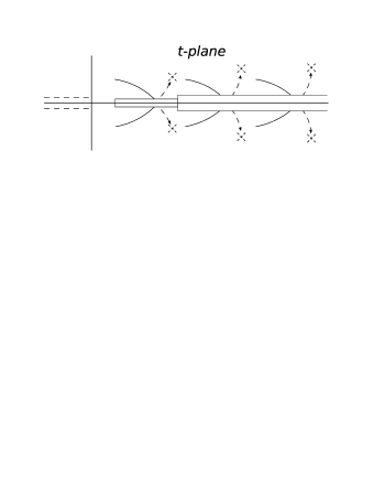
Figure 1: Analytic properties of charged pion EM FF.

Consequently, the $U\&A$ model of meson EM structure takes the form

$$F_{P}[W(t)]=\left(\frac{1-W^{2}}{1-W^{2}_{N}}\right)^{2}\times$$

$$\times\Bigg{\{}\sum_{i}\frac{(W_{N}-W_{i})(W_{N}-W^{*}_{i})(W_{N}-1/W_{i})(W_{N}-1/W^{*}_{i})}{(W-W_{i})(W-W^{*}_{i})(W-1/W_{i})(W-1/W^{*}_{i})}(f_{iPP}/f_{i})+$$

$$+\sum_{j}\frac{(W_{N}-W_{j})(W_{N}-W^{*}_{j})(W_{N}+W_{j})(W_{N}+W^{*}_{j})}{(W-W_{j})(W-W^{*}_{j})(W+W_{j})(W+W^{*}_{j})}(f_{jPP}/f_{j})\Bigg{\}}$$

which is analytic in the whole complex Fig. 1 besides two cuts on the positive real axis.

IV NOW ONE BY ONE

$\pi^{\pm}$: The analytic properties of $F_{\pi}(t)$ are in Fig. 2. In comparison with expression $F_{P}[W(t)]$ there is additional left-hand cut on the II.Riemann sheet.

The latter is explained by the following way. Starting from the elastic unitarity condition for $F_{\pi}(t)$ $\frac{1}{2i}\{F_{\pi}(t+i\varepsilon)-F^{*}_{\pi}(t+i\varepsilon)\}=A^{1*}_{1}(t+i\varepsilon).F_{\pi}(t+i\varepsilon)$ one can derive the expression for pion EM FF on the II.Riemann sheet $[F_{\pi}(t)]^{II.}=\frac{F_{\pi}(t)}{1+2iA^{1}_{1}(t)}$ where $A^{1}_{1}(t)$ is the $P$-wave isovector $\pi\pi$-scattering amplitude, the analytic properties of which consist of right-hand unitary cut $4m^{2}_{\pi}<t<\infty$ and of left-hand dynamical cut $-\infty<t<0.$. Taking into account the fact that the contribution of any cut in Pad’e approximation can be represented by alternating zeros and poles on the place of the cut then we do it in $U\&A$ model of $F_{\pi}[W(t)]$.

From the same elastic unitarity condition and $\delta^{1}_{1}(t)_{q\to 0}\sim a^{1}_{1}q^{3}$ one gets the threshold behavior of $ImF_{\pi}(t)$ to be transformed into 3 threshold conditions $ImF_{\pi}(t)_{q=0}=\frac{dImF_{\pi}(t)}{dq}_{q=0}=\frac{d^{2}ImF_{\pi}(t)}{dq}_{q=0}\equiv 0$, which reduce a number of $(f_{v\pi\pi}/f_{v})$ as free parameters.

Taking into account both these notes and also the normalization explicitly one gets the $U\&A$ pion EM FF model dub

$$F_{\pi}[W(t)]=\left(\frac{1-W^{2}}{1-W^{2}_{N}}\right)^{2}\frac{(W-W_{z})(W_{N}-W_{p})}{(W_{N}-W_{z})(W-W_{p})}\times$$

$$\times\Bigg{\{}\frac{(W_{N}-W_{\rho})(W_{N}-W^{*}_{\rho})(W_{N}-1/W_{\rho})(W_{N}-1/W^{*}_{\rho})}{(W-W_{\rho})(W-W^{*}_{\rho})(W-1/W_{\rho})(W-1/W^{*}_{\rho})}(f_{\rho\pi\pi}/f_{\rho})+$$

$$+\sum\limits_{v=\rho^{\prime},\rho^{\prime\prime}}\frac{(W_{N}-W_{v})(W_{N}-W^{*}_{v})(W_{N}+W_{v})(W_{N}+W^{*}_{v})}{(W-W_{v})(W-W^{*}_{v})(W+W_{v})(W+W^{*}_{v})}(f_{v\pi\pi}/f_{v})\Bigg{\}}$$

with $(f_{\rho^{\prime}\pi\pi}/f_{\rho^{\prime}})=\frac{\frac{N_{\rho^{\prime\prime}}}{\mid W_{\rho^{\prime\prime}}\mid^{4}}}{\frac{N_{\rho^{\prime}}}{\mid W_{\rho^{\prime}}\mid^{4}}-\frac{N_{\rho^{\prime\prime}}}{\mid W_{\rho^{\prime\prime}}\mid^{4}}}-\frac{\frac{N_{\rho^{\prime\prime}}}{\mid W_{\rho^{\prime\prime}}\mid^{4}}+(1+2\frac{W_{z}.W_{p}}{W_{z}-W_{p}}.Re[W_{\rho}(1+\mid W_{\rho}\mid^{-2})])N_{\rho}}{\frac{N_{\rho^{\prime}}}{\mid W_{\rho^{\prime}}\mid^{4}}-\frac{N_{\rho^{\prime\prime}}}{\mid W_{\rho^{\prime\prime}}\mid^{4}}}(f_{\rho\pi\pi}/f_{\rho})$
$(f_{\rho^{\prime\prime}\pi\pi}/f_{\rho^{\prime\prime}})=1-\frac{\frac{N_{\rho^{\prime\prime}}}{\mid W_{\rho^{\prime\prime}}\mid^{4}}}{\frac{N_{\rho^{\prime}}}{\mid W_{\rho^{\prime}}\mid^{4}}-\frac{N_{\rho^{\prime\prime}}}{\mid W_{\rho^{\prime\prime}}\mid^{4}}}+[\frac{\frac{N_{\rho^{\prime\prime}}}{\mid W_{\rho^{\prime\prime}}\mid^{4}}+(1+2\frac{W_{z}.W_{p}}{W_{z}-W_{p}}.Re[W_{\rho}(1+\mid W_{\rho}\mid^{-2})])N_{\rho}}{\frac{N_{\rho^{\prime}}}{\mid W_{\rho^{\prime}}\mid^{4}}-\frac{N_{\rho^{\prime\prime}}}{\mid W_{\rho^{\prime\prime}}\mid^{4}}}-1](f_{\rho\pi\pi}/f_{\rho})$

Due to the $\rho-\omega$ interference effect one has to carry out the fit of existing data by $\mid F_{\pi}[W(t)]+R.e^{i\phi}\frac{m^{2}_{\omega}}{m^{2}_{\omega}-t-im_{\omega}\Gamma_{\omega}}\mid$ with $\phi=arctg\frac{m_{\rho}\Gamma_{\rho}}{m^{2}_{\rho}-m^{2}_{\omega}}$.

A description of existing data in space-like and time-like regions simultaneously with parameters values $t_{in}=(1.296\pm 0.011)GeV^{2}$; $R=0.0123\pm 0.0032$; $W_{z}=0.3722\pm 0.0008$; $W_{p}=0.5518\pm 0.0003$; $m_{\rho}=(759.26\pm 0.04)MeV$; $\Gamma_{\rho}=(141.90\pm 0.13)MeV$; $m_{\rho^{\prime}}=(1395.9\pm 54.3)MeV$; $\Gamma_{\rho^{\prime}}=(490.9\pm 118.8)MeV$ $m_{\rho^{\prime\prime}}=(1711.5\pm 63.6)MeV$; $\Gamma_{\rho^{\prime\prime}}=(369.5\pm 112.7)MeV$; $(f_{\rho\pi\pi}/f_{\rho})=1.0063\pm 0.0024$; $\chi^{2}/ndf=1.58$; is presented in Fig. 2.

Figure 2: Prediction of pion EM FF behavior by $U\&A$ model.

$K^{\pm},K^{0}$:

The $K^{+}$ and $K^{0}$ belong to the same isomultiplet with $I=1/2$. Then one can introduce, generally, the EM current of $K$, which splits into sum of isotopic scalar and isotopic vector.

The corresponding FFs suitable for a construction of the $U\&A$ models are $F^{s}_{K}(t)=\frac{1}{2}[F_{K^{+}}(t)+F_{K^{0}}(t)]$  $F_{K^{+}}(t)=F^{s}_{K}(t)+F^{v}_{K}(t)$
$F^{v}_{K}(t)=\frac{1}{2}[F_{K^{+}}(t)-F_{K^{0}}(t)]$  $F_{K^{0}}(t)=F^{s}_{K}(t)-F^{v}_{K}(t)$
from where the normalizations $F^{s}_{K}(0)=F^{v}_{K}(0)=\frac{1}{2}$;  $F_{K^{+}}(0)=1$;  $F_{K^{0}}(0)=0$; follow. The specific 6 resonance ($\rho,\omega,\phi,\rho^{\prime},\phi^{\prime},\rho^{\prime\prime}$) $U\&A$ model of the kaon EM structure has the form ddl

$$F^{s}_{K}[V(t)]=\Bigg{(}\frac{1-V^{2}}{1-V^{2}_{N}}\Bigg{)}^{2}\Bigg{[}\frac{1}{2}\frac{(V_{N}-V_{\omega})(V_{N}-V^{*}_{\omega})(V_{N}-1/V_{\omega})(V_{N}-1/V^{*}_{\omega})}{(V-V_{\omega})(V-V^{*}_{\omega})(V-1/V_{\omega})(V-1/V^{*}_{\omega})}+$$

$$+\Bigg{\{}\frac{(V_{N}-V_{\phi})(V_{N}-V^{*}_{\phi})(V_{N}-1/V_{\phi})(V_{N}-1/V^{*}_{\phi})}{(V-V_{\phi})(V-V^{*}_{\phi})(V-1/V_{\phi})(V-1/V^{*}_{\phi})}-$$

$$-\frac{(V_{N}-V_{\omega})(V_{N}-V^{*}_{\omega})(V_{N}-1/V_{\omega})(V_{N}-1/V^{*}_{\omega})}{(V-V_{\omega})(V-V^{*}_{\omega})(V-1/V_{\omega})(V-1/V^{*}_{\omega})}\Bigg{\}}(f_{\phi KK}/f_{\phi})+$$ (6)

$$+\Bigg{\{}\frac{(V_{N}-V_{\phi^{\prime}})(V_{N}-V^{*}_{\phi^{\prime}})(V_{N}-1/V_{\phi^{\prime}})(V_{N}-1/V^{*}_{\phi^{\prime}})}{(V-V_{\phi^{\prime}})(V-V^{*}_{\phi^{\prime}})(V-1/V_{\phi^{\prime}})(V-1/V^{*}_{\phi^{\prime}})}-$$

$$-\frac{(V_{N}-V_{\omega})(V_{N}-V^{*}_{\omega})(V_{N}-1/V_{\omega})(V_{N}-1/V^{*}_{\omega})}{(V-V_{\omega})(V-V^{*}_{\omega})(V-1/V_{\omega})(V-1/V^{*}_{\omega})}\Bigg{\}}(f_{\phi^{\prime}KK}/f_{\phi^{\prime}})\Bigg{]}$$

$$F^{v}_{K}[W(t)]=\Bigg{(}\frac{1-W^{2}}{1-W^{2}_{N}}\Bigg{)}^{2}\Bigg{[}\frac{1}{2}\frac{(W_{N}-W_{\rho})(W_{N}-W^{*}_{\rho})(W_{N}-1/W_{\rho})(W_{N}-1/W^{*}_{\rho})}{(W-W_{\rho})(W-W^{*}_{\rho})(W-1/W_{\rho})(W-1/W^{*}_{\rho})}+$$

$$+\Bigg{\{}\frac{(W_{N}-W_{\rho^{\prime}})(W_{N}-W^{*}_{\rho^{\prime}})(W_{N}-1/W_{\rho^{\prime}})(W_{N}-1/W^{*}_{\rho^{\prime}})}{(W-W_{\rho^{\prime}})(W-W^{*}_{\rho^{\prime}})(W-1/W_{\rho^{\prime}})(W-1/W^{*}_{\rho^{\prime}})}-$$

$$-\frac{(W_{N}-W_{\rho})(W_{N}-W^{*}_{\rho})(W_{N}-1/W_{\rho})(W_{N}-1/W^{*}_{\rho})}{(W-W_{\rho})(W-W^{*}_{\rho})(W-1/W_{\rho})(W-1/W^{*}_{\rho})}\Bigg{\}}(f_{\rho^{\prime}KK}/f_{\rho^{\prime}})+$$ (7)

$$+\Bigg{\{}\frac{(W_{N}-W_{\rho^{\prime\prime}})(W_{N}-W^{*}_{\rho^{\prime\prime}})(W_{N}-1/W_{\rho^{\prime\prime}})(W_{N}-1/W^{*}_{\rho^{\prime\prime}})}{(W-W_{\rho^{\prime\prime}})(W-W^{*}_{\rho^{\prime\prime}})(W-1/W_{\rho^{\prime\prime}})(W-1/W^{*}_{\rho^{\prime\prime}})}-$$

$$-\frac{(W_{N}-W_{\rho})(W_{N}-W^{*}_{\rho})(W_{N}-1/W_{\rho})(W_{N}-1/W^{*}_{\rho})}{(W-W_{\rho})(W-W^{*}_{\rho})(W-1/W_{\rho})(W-1/W^{*}_{\rho})}\Bigg{\}}(f_{\rho^{\prime\prime}KK}/f_{\rho^{\prime\prime}})\Bigg{]}$$

Both functions are analytic in the whole complex $t$-planes besides two cuts on the positive real axis, generated by $t^{s}_{0}=9m^{2}_{\pi}$ and $t^{s}_{in}$ in $F^{s}_{K}[V(t)]$ and by $t^{v}_{0}=4m^{2}_{\pi}$ and $t_{in}$ in $F^{v}_{K}[W(t)]$. They are real on the whole real negative axis up to positive values $t^{s}_{0}=9m^{2}_{\pi}$ and $t^{v}_{0}=4m^{2}_{\pi}$, respectively, automatically normalized to $1/2$ with $ImF^{s}_{K}(t)\neq 0$ and $ImF^{v}_{K}(t)\neq 0$, starting from $9m^{2}_{\pi}$ and $4m^{2}_{\pi}$, respectively, as it is required by the unitarity conditions. They possess complex conjugate pairs of poles on unphysical sheets of the Riemann surface, corresponding to considered vector-mesons with quantum numbers of the photon.

A simultaneous reproduction of all existing kaon EM FF data by the $U\&A$ models is presented in Fig. 3 and Fig. 4

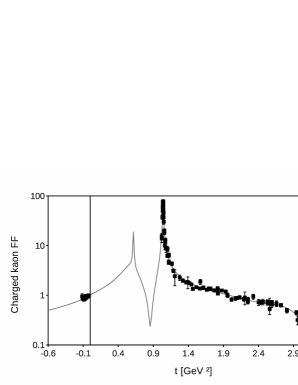
Figure 3: Prediction of charge kaon EM FF behavior by $U\&A$ model.

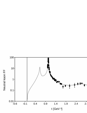
Figure 4: Prediction of neutral kaon EM FF behavior by $U\&A$ model.

and the following values of free parameters of the model have been determined - $m_{\rho},\Gamma_{\rho},m_{\omega},\Gamma_{\omega}$ are fixed at the TABLE values. $q^{s}_{in}=\sqrt{(t^{s}_{in}-9)/9}=2.2326[m_{\pi}]$; $q^{v}_{in}=\sqrt{(t^{v}_{in}-4)/4}=6.6721[m_{\pi}]$; $(f_{\omega KK}/f_{\omega})=0.14194$; $(f_{\rho KK}/f_{\rho})=0.5615$;
$m_{\phi}=7.2815[m_{\pi}]$; $m_{\rho^{\prime}}=10.3940[m_{\pi}]$; $\Gamma_{\phi}=0.03733[m_{\pi}]$; $\Gamma_{\rho^{\prime}}=1.6284[m_{\pi}]$;
$(f_{\phi KK}/f_{\phi})=0.4002$; $(f_{\rho^{\prime}KK}/f_{\rho^{\prime}})=-.3262$;
$m_{\phi^{\prime}}=11.8700[m_{\pi}]$; $m_{\rho^{\prime\prime}}=13.5650[m_{\pi}]$; $\Gamma_{\phi^{\prime}}=1.3834[m_{\pi}]$; $\Gamma_{\rho^{\prime\prime}}=3.3313[m_{\pi}]$;
$(f_{\phi^{\prime}KK}/f_{\phi^{\prime}})=-.04214$; $(f_{\rho^{\prime\prime}KK}/f_{\rho^{\prime\prime}})=-.02888$

What about $\pi^{0},\eta,\eta^{\prime}$:

They are true neutral particles and then their elastic EM FFs $F_{\pi^{0}}(t)=0$; $F_{\eta}(t)=0$; $F_{\eta^{\prime}}(t)=0$ i.e. these particles are point-like according to EM interactions.

However, one can define nonzero single FF for each $\gamma^{*}\to\gamma P$ transition by a parametrization of the matrix element of the EM current $<P(p)\mid J^{EM}_{\mu}\mid 0>=\varepsilon_{\mu\nu\alpha\beta}p^{\nu}\epsilon^{\alpha}k^{\beta}F_{\gamma P}(q^{2})$ with $\epsilon^{\alpha}$ to be the polarization vector of $\gamma$, and $\varepsilon_{\mu\nu\alpha\beta}$ is antisymmetric tensor.

The transition FFs are related to corresponding cross sections
$\sigma_{tot}(e^{+}e^{-}\to P\gamma)=\frac{\pi\alpha^{2}}{6}(1-\frac{m^{2}_{P}}{t})^{3}\mid F_{P\gamma}(t)\mid^{2}$
giving experimental data on $F_{\pi^{0}\gamma}(t),F_{\eta\gamma}(t)$ and $F_{\eta^{\prime}\gamma}(t)$ in $t>0$ region.

A straightforward calculation of $F_{P\gamma}(t)$ in $QCD$ is impossible. One has to construct sophisticated phenomenological models.

In a construction of the $U\&A$ model it is again suitable to split $F_{P\gamma}(t)$ into two terms depending on the isotopic character of the photon $F_{P\gamma}(t)=F^{I=0}_{P\gamma}(t)+F^{I=1}_{P\gamma}(t)$ where $F^{I=0}_{P\gamma}(t)$ is saturated by isoscalar vector-mesons $\omega,\phi,\omega^{\prime},\phi^{\prime}$ etc. and $F^{I=1}_{P\gamma}(t)$ is saturated by isovector vector-mesons $\rho,\rho^{\prime},\rho^{\prime\prime}$ etc. However, there is a question how many vector-meson resonances have to be taken into account. It is prescribed by the existing data interval on the corresponding FF in $t>0$ region.

The data on $\pi^{0}\gamma$ transition FF allow to consider all $3$ ground state vector mesons, $\rho(770),\omega(782),\phi(1020)$ and also $\omega^{\prime}(1420)$ and $\rho^{\prime}(1450)$, in order to construct automatically normalized $U\&A$ models.

With the aim of obtaining comparable results, the same number of resonances is considered also for $\eta$ and $\eta^{\prime}$.

In the analysis the resonance parameters are fixed at the TABLE values, the normalization of FFs are $F_{P\gamma}(0)=\frac{2}{\alpha m_{P}}\sqrt{\frac{\Gamma(P\to\gamma\gamma)}{\pi m_{P}}}$ where $\Gamma(P\to\gamma\gamma)$ are fixed at the world averaged values from TABLE.

The $F_{P\gamma}(t)$ FFs are analytic in $t$ - plane besides the cut from $t=m^{2}_{\pi^{0}}$ up to $+\infty$. Then the $U\&A$ model of $F_{P\gamma}(t)$ takes the form ddl2
$F^{I=0}_{P\gamma}[V(t)]=\Bigg{(}\frac{1-V^{2}}{1-V^{2}_{N}}\Bigg{)}^{2}{\frac{1}{2}F_{P\gamma}(0)H(\omega^{\prime})+[L(\omega)-H(\omega^{\prime})]a_{\omega}+[H(\phi)-H(\omega^{\prime})]a_{\phi}\}}$
$F^{I=1}_{P\gamma}[W(t)]=\Bigg{(}\frac{1-W^{2}}{1-W^{2}_{N}}\Bigg{)}^{2}\{\frac{1}{2}F_{P\gamma}(0)H(\rho^{\prime})+[L(\rho)-H(\rho^{\prime})]a_{\rho}\}$
with $L(\omega)=\frac{(V_{N}-V_{\omega})(V_{N}-V^{*}_{\omega})(V_{N}-1/V_{\omega})(V_{N}-1/V^{*}_{\omega})}{(V-V_{\omega})(V-V^{*}_{\omega})(V-1/V_{\omega})(V-1/V^{*}_{\omega})}$; $H(i)=\frac{(V_{N}-V_{i})(V_{N}-V^{*}_{i})(V_{N}+V_{i})(V_{N}+V^{*}_{i})}{(V-V_{i})(V-V^{*}_{i})(V+V_{i})(V+V^{*}_{i})}$; $i=\phi,\omega^{\prime}$

$L(\rho)=\frac{(W_{N}-W_{\rho})(W_{N}-W^{*}_{\rho})(W_{N}-1/W_{\rho})(W_{N}-1/W^{*}_{\rho})}{(W-W_{\rho})(W-W^{*}_{\rho})(W-1/W_{\rho})(W-1/W^{*}_{\rho})}$; $H(\rho^{\prime})=\frac{(W_{N}-W_{\rho^{\prime}})(W_{N}-W^{*}_{\rho^{\prime}})(W_{N}+W_{\rho^{\prime}})(W_{N}+W^{*}_{\rho^{\prime}})}{(W-W_{\rho^{\prime}})(W-W^{*}_{\rho^{\prime}})(W+W_{\rho^{\prime}})(W+W^{*}_{\rho^{\prime}})}$

and the normalization points $V(0)=V_{N},$  $W(0)=W_{N}$.

The model depends on $5$ free parameters $t^{s}_{in},t^{v}_{in},a_{j}=(f_{\gamma Pj}/f_{j}),$  $j=\rho,\omega,\phi$ determined in an optimal description of existing data.

for $\pi^{0}$: see Fig. 5

$q^{s}_{in}=5.5210\pm 0.0084$; $q^{v}_{in}=5.61220\pm 0.1414$; $a_{\omega}=0.0063\pm 0.0013$;
$a_{\rho}=0.0212\pm 0.0006$; $a_{\phi}=-.0004\pm 0.0001$; $\chi^{2}/ndf=121/75=1.61$

Figure 5: Prediction of $\pi^{0}\gamma$ transition EM FF behavior by $U\&A$ model.

Figure 6: Prediction of $\eta\gamma$ transition EM FF behavior by $U\&A$ model.

Figure 7: Prediction of $\eta^{\prime}\gamma$ transition EM FF behavior by $U\&A$ model.

for $\eta$: see Fig. 6

$q^{s}_{in}=6.7104\pm 0.0190$; $q^{v}_{in}=5.5006\pm 0.0632$; $a_{\omega}=0.0002\pm 0.0014$;
$a_{\rho}=0.0250\pm 0.0013$; $a_{\phi}=-.0020\pm 0.0003$; $\chi^{2}/ndf=52/52=1.00$

for $\eta^{\prime}$: see Fig. 7

$q^{s}_{in}=5.5366\pm 0.0891$; $q^{v}_{in}=7.7554\pm 0.0158$; $a_{\omega}=-.1134\pm 0.0078$;
$a_{\rho}=0.1241\pm 0.0026$; $a_{\phi}=0.0098\pm 0.0091$; $\chi^{2}/ndf=59/50=1.18$

V CONCLUSIONS

We have investigated EM structure of pseudoscalar mesons to be described by the corresponding EM FFs. Since there is no possibility to describe the latter in the framework of $QCD$, the universal $U\&A$ models have been elaborated.

More or less successful description of all existing data on the whole complete nonet of pseudoscalar mesons $\pi^{-},\pi^{0},\pi^{+},K^{-},K^{0},\bar{K}^{0},K^{+},\eta,\eta^{\prime}$ has been achieved in space-like and time-like regions simultaneously.

The work was supported in part by Slovak Grant Agency for Sciences VEGA, Grant 2/0009/10.

References

• (1) K.Nakamura et al (Particle Data Group), J. Phys G37 (2010) 075021
• (2) S.Dubnicka, A.Z.Dubnickova, Acta Phys. Slovaca 60 (2010) 1
• (3) S.Dubnicka, $\pi N$ Newsletter 11 (1995) 167
• (4) S.Dubnicka, A.Z.Dubnickova, A.Liptaj, Nucl. Phys. B (Proc. Suppl.) 219-220 (2011) 271
• (5) S.Dubnicka, A.Z.Dubnickova, A.Liptaj, Prog. Part. Nucl. Phys, 67 (2012) 418