Two-dimensional Potts antiferromagnets with a phase transition at arbitrarily large $\bm{q}$

Abstract

We exhibit infinite families of two-dimensional lattices (some of which are triangulations or quadrangulations of the plane) on which the $q$-state Potts antiferromagnet has a finite-temperature phase transition at arbitrarily large values of $q$. This unexpected result is proven rigorously by using a Peierls argument to measure the entropic advantage of sublattice long-range order. Additional numerical data are obtained using transfer matrices, Monte Carlo simulation, and a high-precision graph-theoretic method.

The $q$-state Potts model Potts_52 ; Wu_82+84 plays an important role in the theory of critical phenomena, especially in two dimensions (2D) Baxter_book ; Nienhuis_84 ; DiFrancesco_97 , and has applications to various condensed-matter systems Wu_82+84 . Ferromagnetic Potts models are by now fairly well understood, thanks to universality; but the behavior of antiferromagnetic Potts models depends strongly on the microscopic lattice structure, so that many basic questions about the phase diagram and critical exponents must be investigated case-by-case. In this article we prove the unexpected existence of phase transitions for some 2D $q$-state Potts antiferromagnets at arbitrarily large values of $q$.

For Potts antiferromagnets one expects that for each lattice ${\cal L}$ there is a value $q_{c}({\cal L})$ [possibly noninteger] such that for $q>q_{c}({\cal L})$ the model has exponential decay of correlations at all temperatures including zero, while for $q=q_{c}({\cal L})$ there is a zero-temperature critical point. The first task, for any lattice, is thus to determine $q_{c}$.

Some 2D antiferromagnetic models at zero temperature can be mapped exactly onto a “height” model Salas_98 ; Jacobsen_09 . Since the height model must either be in a “smooth” (ordered) or “rough” (massless) phase, the corresponding zero-temperature spin model must either be ordered or critical, never disordered. Until now it has seemed that the most common case is criticality height_rep_exceptions .

In particular, when the $q$-state zero-temperature Potts antiferromagnet (AF) on a 2D lattice ${\cal L}$ admits a height representation, one ordinarily expects that $q=q_{c}({\cal L})$. This prediction is confirmed in most heretofore-studied cases: 3-state square-lattice Nijs_82 ; Kolafa_84 ; Burton_Henley_97 ; Salas_98 , 3-state kagome Huse_92 ; Kondev_96 , 4-state triangular Moore_00 , and 4-state on the line graph of the square lattice Kondev_95 ; Kondev_96 . Until recently the only known exception was the triangular Ising AF note_TRI_q=2 .

Kotecký, Salas and Sokal (KSS) Kotecky-Salas-Sokal observed that the height mapping employed for the 3-state Potts AF on the square lattice Salas_98 carries over unchanged to any plane quadrangulation; and Moore and Newman Moore_00 observed that the height mapping employed for the 4-state Potts AF on the triangular lattice carries over unchanged to any Eulerian plane triangulation (a graph is called Eulerian if all vertices have even degree). One therefore expects naively that $q_{c}=3$ for every (periodic) plane quadrangulation, and that $q_{c}=4$ for every (periodic) Eulerian plane triangulation.

Surprisingly, these predictions are false! KSS Kotecky-Salas-Sokal proved rigorously that the 3-state AF on the diced lattice (which is a quadrangulation) has a phase transition at finite temperature (see also Kotecky-Sokal-Swart ); numerical estimates from transfer matrices yield $q_{c}({\rm diced})\approx 3.45$ Jacobsen-Salas_unpub . Likewise, we recently union-jack provided analytic arguments (falling short, however, of a rigorous proof) that on any Eulerian plane triangulation in which one sublattice consists entirely of vertices of degree 4, the 4-state AF has a phase transition at finite temperature, so that $q_{c}>4$. We also presented transfer-matrix and Monte Carlo data confirming these predictions for the union-jack and bisected hexagonal lattices, leading to the estimates $q_{c}({\rm UJ})\approx 4.33$ and $q_{c}({\rm BH})\approx 5.40$.

These results suggest the obvious question: How large can $q_{c}$ be on a plane quadrangulation (resp. Eulerian plane triangulation)? The answers are clearly larger than 3 or 4, respectively — but how much larger?

In this article we shall give a rigorous proof of the unexpected answer: we exhibit infinite classes of plane quadrangulations and Eulerian plane triangulations on which $q_{c}$ can take arbitrarily large values. We shall also complement this rigorous proof with detailed quantitative data from transfer matrices, Monte Carlo simulations, and a powerful graph-theoretic approach developed recently by Jacobsen and Scullard JS1 .

The models studied here provide new examples of entropically-driven long-range order Kotecky-Salas-Sokal ; union-jack ; Kotecky-Sokal-Swart ; Chen_11 : the ferromagnetic ordering of spins on one sublattice is favored because it increases the freedom of choice of spins on the other sublattice(s). But though this idea is intuitively appealing, it is usually difficult to determine quantitatively, in any specific case, whether the entropic penalty for interfaces between domains of differently-ordered spins on the first sublattice is large enough to produce long-range order. Moreover, one expects that this penalty decreases with increasing $q$. In the examples given here, by contrast, we are able to prove that the penalty can be made arbitrarily strong and hence operative at arbitrarily large $q$.

The lattices $G_{n}$ and $H_{n}$.

Let $G_{n}$ be obtained from the square (SQ) lattice by replacing each edge with $n$ two-edge paths in parallel; and let $H_{n}$ be obtained from $G_{n}$ by connecting each group of $n$ “new” vertices with an $(n-1)$-edge path (see Fig. 1). Resumming over the spins on the “new” vertices Sokal_bcc2005 , it is easy to show that the $q$-state Potts model on $G_{n}$ or $H_{n}$ with nearest-neighbor coupling $v=e^{J}-1$ is equivalent to a SQ-lattice Potts model with a suitable coupling $v_{\rm eff}(q,v)$ Kotecky_85 ; moreover, for $q>2$ (resp. $q>3$) an AF model ($-1\leq v\leq 0$) on $G_{n}$ (resp. $H_{n}$) maps onto a ferromagnetic model ($v_{\rm eff}\geq 0$) on the SQ lattice. Concretely, for the zero-temperature AF ($v=-1$) we have

$$v_{\rm eff}^{G_{n}}(q,-1) \>=\> \Bigl{(}{q-1\over q-2}\Bigr{)}^{n}\,-\,1$$ (1)

$$v_{\rm eff}^{H_{n}}(q,-1) \>=\> {q-1\over q-2}\,\Bigl{(}{q-2\over q-3}\Bigr{)}^{n-1}\,-\,1$$ (2)

Setting $v_{\rm eff}$ equal to the SQ-lattice ferromagnetic critical point $v_{c}({\rm SQ})=\sqrt{q}$ Baxter_book ; Beffara_12 , we obtain $q_{c}$ for $G_{n}$ and $H_{n}$; they have the large-$n$ asymptotic behavior

$$q_{c}(G_{n})\>\approx\>q_{c}(H_{n})\;\approx\;{2n\over W(2n)}\,+\,O\bigl{(}(n/\log n)^{1/2}\bigr{)}$$ (3)

where $W(x)\approx\log x-\log\log x+o(1)$ is the Lambert $W$ function note_Lambert . We have thus exhibited two infinite families of periodic planar lattices on which the Potts AF has arbitrarily large $q_{c}$ as $n\to\infty$ note_KSS . These lattices are not triangulations or quadrangulations, but they can be modified to be such and retain the phase transition, as we now show.

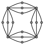
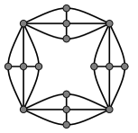
(a)		(b)

Figure 1: Unit cells of the lattices $G_{n}$ (a) and $H_{n}$ (b) for $n=3$.

The modified lattices.

Starting from $G_{n}$ or $H_{n}$, insert a new vertex into each octagonal face and connect it either to the four surrounding vertices of the original SQ lattice, to the four “new” vertices, or to all eight vertices; call these modifications ^′, ^′′ and ^′′′, respectively. In particular, $G^{\prime}_{n}$ and $G^{\prime\prime}_{n}$ are quadrangulations, and $H^{\prime\prime\prime}_{n}$ is an Eulerian triangulation (Fig. 2).

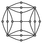
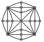
(a)	(b)	(c)

Figure 2: Unit cells of the lattices $G^{\prime}_{n}$ (a), $G^{\prime\prime}_{n}$ (b) and $H^{\prime\prime\prime}_{n}$ (c) for $n=3$.

If we integrate out the spins at the vertices placed into the octagonal faces, we obtain the model on $G_{n}$ or $H_{n}$ perturbed by a 4-spin or 8-spin interaction. When $q$ is large, this interaction is weak (of order $1/q$) because its Boltzmann weight is bounded between a maximum value of $q$ and a minimum value of $q-4$ or $q-8$. We therefore expect that the new edges will have a negligible effect on the phase transition when $q$ is large, and that all the modified lattices will have $q_{c}(n)$ whose large-$n$ behavior is essentially identical to Eq. (3). Let us now sketch a rigorous proof KSS_in_prep of this assertion.

Proof of phase transition.

Recall first how one proves, using the Peierls argument, the existence of ferromagnetic long-range order (FLRO) at low temperature in the $q$-state Potts ferromagnet on the SQ lattice. The Peierls contours are defined as the connected components of the union of all bonds on the dual SQ lattice that separate unequal spins. A Peierls contour $\gamma$ of length $|\gamma|$ and cyclomatic number $c(\gamma)$ comes with a weight that is bounded above by $(q-1)^{c(\gamma)}(1+v)^{-|\gamma|}$: here $(q-1)^{c(\gamma)}$ is a bound on the number of colorings of the SQ lattice consistent with the contour $\gamma$. Further, on the SQ lattice we have $c(\gamma)\leq|\gamma|/2$, and the number of contours of length $n$ surrounding a fixed site can be bounded by $(n/2)16^{n}$. Standard Peierls reasoning then shows that for any pair of sites $x,y$ one has

$$\hbox{Prob}(\sigma_{x}\neq\sigma_{y})\;\leq\;\sum_{n=4}^{\infty}(n/2)16^{n}(q-1)^{n/2}(1+v)^{-n}\,,\;$$ (4)

which is $\leq 5/16$ whenever $1+v\geq 32\sqrt{q}$. This proves FLRO (the constant 32 is of course suboptimal). The foregoing argument is valid for fixed boundary conditions (e.g., $\sigma=1$) in the plane, but with suitable modifications it can also be carried out for periodic boundary conditions (i.e., on a torus).

Let us now consider the Potts antiferromagnet on one of the six modified lattices $G^{\prime}_{n},\ldots,H^{\prime\prime\prime}_{n}$. Since our goal is to show FLRO on the SQ sublattice, we define Peierls contours exactly as we did for the SQ-lattice ferromagnet, ignoring the spin values at all other sites. Although we no longer have any simple explicit formula for the contour weights, it is nevertheless possible to prove an upper bound on the probability of occurrence of a contour $\gamma$ by using the technique of reflection positivity and chessboard estimates chessboard_papers . Without going into details of the needed adaptations of this standard technique for our case (see KSS_in_prep ), we mention only that the final bound on the probability of occurrence of a contour $\gamma$ is $(\kappa\sqrt{q-1})^{|\gamma|}$, where $\kappa$ is the probability that the spins on the SQ sublattice follow a fixed checkerboard pattern (say, 1 on the even sublattice and 2 on the odd sublattice) raised to the power 1/volume. This latter probability is easy to bound explicitly, yielding $\kappa\leq[1+v_{\rm eff}(q,v)]^{-1}[q/(q-5)]^{1/2}$, where $v_{\rm eff}(q,v)$ is the one for the corresponding unmodified lattice $G_{n}$ or $H_{n}$. This implies that, for all the lattices $G^{\prime}_{n},\ldots,H^{\prime\prime\prime}_{n}$, there is FLRO on the SQ sublattice whenever $6\leq q\leq q_{c}(G_{n})-O(1)$ [cf. Eq. (3)] and $v$ is close to $-1$ (low temperature).

Let us also remark that the lattice $G^{\prime\prime}_{2}$ is covered by the general theory of Kotecky-Sokal-Swart , where it is proven that $q_{c}>3$; moreover, a minor modification proves the same result for $G^{\prime\prime}_{n}$ for all $n\geq 2$.

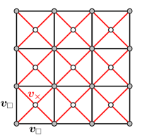
Figure 3: (Color online) The union-jack (UJ) lattice.

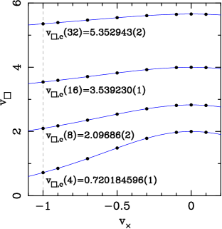
Figure 4: (Color online) Estimated phase boundaries for the $q=4,8,16,32$ Potts models on the union-jack (UJ) lattice, from the Jacobsen–Scullard method (blue curve and numerical values of $v_{\Box,{\rm c}}$ at $v_{\times}=-1$) and Monte Carlo simulations (black points).

$\;n\;$	$q_{c}(G_{n})$	$q_{c}(G^{\prime}_{n})$	$q_{c}(H_{n})$	$q_{c}(H^{\prime}_{n})$	$2n/W(2n)$
	(exact)	(JS)	(exact)	(JS)	(asymp.)
1	2.618034	3.74583(8)	2.618034	3.74583(8)	2.345751
2	3.448678	4.48805(4)	4.000000	4.80794(5)	3.327322
4	4.942152	5.87902(5)	5.617069	6.39269(4)	4.981903
8	7.565625	8.40372(3)	8.304127	9.04238(2)	7.792741
16	12.164794	12.91503(1)	12.939420	13.63221(2)	12.621338
32	20.270897	20.945341(3)	21.068717	21.711603(3)	21.016077
64	34.667189	35.276721(3)	35.482095	36.074775(3)	35.780223

Table 1: Estimates of $q_{c}(n)$ for the lattices $G_{n},G^{\prime}_{n},H_{n},H^{\prime}_{n}$ from the Jacobsen–Scullard (JS) method or the exact solution, and their large-$n$ asymptote $2n/W(2n)$ from Eq. (3).

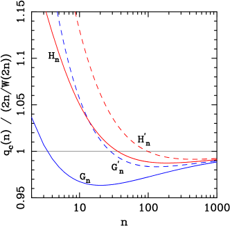
Figure 5: (Color online) Estimates of $q_{c}(n)$ for the lattices $G_{n},G^{\prime}_{n},H_{n},H^{\prime}_{n}$ divided by their large-$n$ asymptote $2n/W(2n)$.

Data for lattices $G^{\prime}_{n}$ and $H^{\prime}_{n}$.

The lattices $G^{\prime}_{n}$ and $H^{\prime}_{n}$ for all $n$ can be reduced to the union-jack (UJ) lattice (Fig. 3) with $v_{\times}=v$ and $v_{\Box}=$ a suitable $v_{\rm eff}(q,v)$ [cf. Eqns. (1)/(2) when $v=-1$]; of course the same reduction holds for $G_{n}$ and $H_{n}$ by setting $v_{\times}=0$. We obtained high-precision estimates of the phase boundary of the UJ model in the $(v_{\times},v_{\Box})$-plane by using the Jacobsen–Scullard (JS) method JS1 with untwisted square bases of size up to $7\times 7$ (294 edges) JS2 . We checked these results for $q=4,8,16,32$ by Monte Carlo simulations using a cluster algorithm note_algorithm . The estimated phase boundaries from both methods are shown in Fig. 4, along with the numerical estimates of $v_{\Box,{\rm c}}$ at $v_{\times}=-1$ from the JS method. The estimates of $q_{c}(n)$ for the lattices $G_{n},G^{\prime}_{n},H_{n},H^{\prime}_{n}$ from the JS method (or the exact solution) are shown in Table 1, where they are compared with the predicted large-$n$ asymptote $q_{c}(n)\approx 2n/W(2n)$ from Eq. (3). The functions $q_{c}(n)$ divided by $2n/W(2n)$ are plotted in Fig. 5. Note that $q_{c}(G^{\prime}_{n})>q_{c}(G_{n})$ and $q_{c}(H^{\prime}_{n})>q_{c}(H_{n})$, in accordance with the intuitive idea that the AF edges associated to the modification $\,{}^{\prime}\,$ enhance the ferromagnetic ordering on the SQ sublattice note_corrineq .

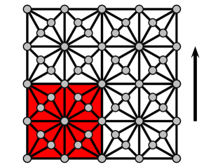
Figure 6: (Color online) The lattice $H^{\prime\prime\prime}_{2}$ (rotated $45^{\circ}$ from Fig. 2) with $L=2$; a unit cell is shown in red, and the transfer direction is indicated with an arrow.

Data for lattices $G^{\prime\prime}_{n}$ and $H^{\prime\prime\prime}_{n}$.

We studied the lattices $G^{\prime\prime}_{n}$ and $H^{\prime\prime\prime}_{n}$ for $n=1,2,4,8,16,32,64$ (note that $G^{\prime\prime}_{1}=$ SQ Salas_98 and $H^{\prime\prime\prime}_{1}=$ UJ union-jack ) at $v=-1$, using transfer matrices with cylindrical boundary conditions on widths $L=1,2,3,4$ unit cells (Fig. 6). The computational complexity is linear in $n$. We estimated the location of the phase transition (which we expect to be first-order whenever $q_{c}>4$) using the crossings of the energies $E_{L}(q)$ Borgs_91 : the results are shown in Table 2.

For $H^{\prime\prime\prime}_{n}$ we checked these results by Monte Carlo: for three integer values of $q$ below the estimated $q_{c}$ we simulated the model at finite temperature and estimated the transition point $v_{c}(q)$; we then performed linear and quadratic extrapolations to locate the point $q_{c}$ where $v_{c}=-1$. The results are shown in Table 2 and Fig. 7 and agree well with the transfer-matrix estimates. For $q\mathrel{\hbox to0.0pt{\lower 3.0pt\hbox{$\mathchar 536\relax$}\hss}\raise 2.0pt\hbox{$\mathchar 318\relax$}}8$ the specific heat diverges at the transition point like $L^{\approx 2}$, in agreement with the finite-size-scaling prediction for a first-order transition; for $4<q\mathrel{\hbox to0.0pt{\lower 3.0pt\hbox{$\mathchar 536\relax$}\hss}\raise 2.0pt\hbox{$\mathchar 316\relax$}}8$ the transition is presumably also first-order but with a large correlation length $\xi$, so that we are unable to observe the true $L\gg\xi$ asymptotic behavior.

Conclusion.

When a 2D model admits a height representation, it must be either critical or ordered. Until now criticality seemed to be the most common case, even though examples of order were known. But here we have exhibited several infinite families of 2D lattices — some of which are quadrangulations or Eulerian triangulations — in which the Potts antiferromagnet admitting a height representation ($q=3$ or 4, respectively) is not only ordered but is in fact “arbitrarily strongly ordered” in the sense that $q_{c}$ is arbitrarily large. This unexpected result suggests that the prior belief may have things precisely backwards. Perhaps criticality is an exceptional case — arising, for instance, in situations with special symmetries — and order is to be generically expected. A key open question raised by this work is to understand why criticality arises when it does.

$\;n\;$	$\>q_{c}(G^{\prime\prime}_{n})\>$	$\>q_{c}(H^{\prime\prime\prime}_{n})\>$	$\>q_{c}(H^{\prime\prime\prime}_{n})\>$	$\,2n/W(2n)\,$
	(TM)	(TM)	(MC)	(asymp.)
1	3.00(0)	4.31(3)		2.345751
2	3.63(2)	5.27(1)	5.26(2)	3.327322
4	5.02(1)	6.68(1)	6.67(3)	4.981903
8	7.60(1)	9.21(1)	9.21(7)	7.792741
16	12.18(2)	13.73(2)	13.73(10)	12.621338
32	20.29(3)	21.76(3)	21.76(32)	21.016077
64	34.70(5)	36.10(5)	36.14(8)	35.780223

Table 2: Estimates of $q_{c}$ for the lattices $G^{\prime\prime}_{n}$ and $H^{\prime\prime\prime}_{n}$ from transfer matrices (TM) and Monte Carlo (MC), and their large-$n$ asymptote from Eq. (3).

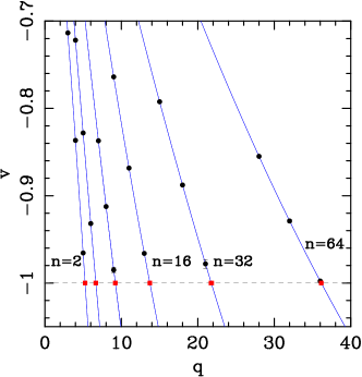
Figure 7: (Color online) Monte Carlo estimates of $v_{c}$ for the lattices $H^{\prime\prime\prime}_{n}$ (black points) and their quadratic fit (blue curves), together with the extrapolated values $q_{c}$ (red squares).

- (1) R.B. Potts, Proc. Cambridge Philos. Soc. 48, 106 (1952).
- (2) F.Y. Wu, Rev. Mod. Phys. 54, 235 (1982); 55, 315 (E) (1983); F.Y. Wu, J. Appl. Phys. 55, 2421 (1984).
- (3) R.J. Baxter, Exactly Solved Models in Statistical Mechanics (Academic Press, London–New York, 1982).
- (4) B. Nienhuis, J. Stat. Phys. 34, 731 (1984).
- (5) P. Di Francesco, P. Mathieu and D. Sénéchal, Conformal Field Theory (Springer-Verlag, New York, 1997).
- (6) J. Salas and A.D. Sokal, J. Stat. Phys 92, 729 (1998), cond-mat/9801079 and the references cited there.
- (7) J.L. Jacobsen, in Polygons, Polyominoes and Polycubes, edited by A.J. Guttmann, Lecture Notes in Physics #775 (Springer, Dordrecht, 2009), Chapter 14.
- (8) Some exceptions are the constrained square-lattice 4-state Potts antiferromagnet Burton_Henley_97 , the triangular-lattice antiferromagnetic spin- Ising model for large enough [C. Zeng and C.L. Henley, Phys. Rev. B 55, 14935 (1997), cond-mat/9609007], the diced-lattice 3-state Potts antiferromagnet Kotecky-Salas-Sokal , and the union-jack and bisected-hexagonal 4-state Potts antiferromagnets union-jack , all of which appear to lie in a non-critical ordered phase at zero temperature.
- (9) J.K. Burton Jr. and C.L. Henley, J. Phys. A: Math. Gen. 30, 8385 (1997), cond-mat/9708171.
- (10) R. Kotecký, J. Salas and A.D. Sokal, Phys. Rev. Lett. 101, 030601 (2008), arXiv:0802.2270.
- (11) Y. Deng, Y. Huang, J.L. Jacobsen, J. Salas and A.D. Sokal, Phys. Rev. Lett. 107, 150601 (2011), arXiv:1108.1743.
- (12) M.P.M. den Nijs, M.P. Nightingale and M. Schick, Phys. Rev. B 26, 2490 (1982).
- (13) J. Kolafa, J. Phys. A: Math. Gen. 17, L777 (1984).
- (14) D.A. Huse and A.D. Rutenberg, Phys. Rev. B 45, 7536 (1992).
- (15) J. Kondev and C.L. Henley, Nucl. Phys. B 464, 540 (1996), cond-mat/9511102.
- (16) C. Moore and M.E.J. Newman, J. Stat. Phys. 99, 629 (2000), cond-mat/9902295.
- (17) J. Kondev and C.L. Henley, Phys. Rev. B 52, 6628 (1995); J.L. Jacobsen and J. Kondev, Nucl. Phys. B 532, 635 (1998), cond-mat/9804048.
- (18) On the triangular lattice, both and are critical at zero temperature and have height representations Blote_82_etc Moore_00 , but .
- (19) H.W.J. Blöte and H.J. Hilhorst, J. Phys. A 15, L631 (1982); B. Nienhuis, H.J. Hilhorst and H.W.J. Blöte, J. Phys. A 17, 3559 (1984).
- (20) R. Kotecký, A.D. Sokal and J.M. Swart, arXiv:1205.4472.
- (21) J.L. Jacobsen and J. Salas, unpublished (2008).
- (22) J.L. Jacobsen and C.R. Scullard, J. Phys. A 45, 494003 (2012), arXiv:1204.0622; C.R. Scullard and J.L. Jacobsen, J. Phys. A 45, 494004 (2012), arXiv:1209.1451; J.L. Jacobsen and C.R. Scullard, J. Phys. A (in press), arXiv:1211.4335.
- (23) Q.N. Chen, M.P. Qin, J. Chen, Z.C. Wei, H.H. Zhao, B. Normand and T. Xiang, Phys. Rev. Lett. 107, 165701 (2011), arXiv:1105.5030.
- (24) This is a special case of the Potts reduction formulae for 2-rooted subgraphs: see A.D. Sokal, in Surveys in Combinatorics, 2005, ed. B.S. Webb (Cambridge University Press, 2005), math.CO/0503607, Section 4.6.
- (25) This equivalence was already observed in R. Kotecký, Phys. Rev. B 31, 3088 (1985) for the -dimensional version of the lattice and used to show the long-range order for and .
- (26) V. Beffara and H. Duminil-Copin, Probab. Th. Rel. Fields 153, 511 (2012), arXiv:1006.5073.
- (27) This function is defined by : see R.M. Corless et al., Adv. Comput. Math. 5, 329 (1996).
- (28) A more complicated example with this property was given in the last paragraph of Kotecky-Salas-Sokal .
- (29) R. Kotecký, A.D. Sokal and J.M. Swart, in preparation.
- (30) J. Fröhlich and E.H. Lieb, Commun. Math. Phys. 60, 233 (1978); J. Fröhlich, R. Israel, E.H. Lieb and B. Simon, Commun. Math. Phys. 62, 1 (1978); M. Biskup, in Methods of Contemporary Mathematical Statistical Physics, ed. R. Kotecký (Springer, Berlin, 2009), math-ph/0610025.
- (31) We performed these computations for symbolic on bases up to (54 edges), numerically for selected triplets near the phase boundary on bases up to (216 edges), and numerically for , , on bases up to (294 edges). These results were made possible by an improvement of the transfer-matrix method of JS1 (J.L. Jacobsen, unpublished).
- (32) The algorithm chooses randomly two of the colors and then simulates the induced mixed ferromagnetic-antiferromagnetic (F–AF) Ising model by the Swendsen–Wang algorithm [R.H. Swendsen and J.-S. Wang, Phys. Rev. Lett. 58, 86 (1987)]. This is a slight extension of the WSK algorithm [J.-S. Wang, R.H. Swendsen and R. Kotecký, Phys. Rev. Lett. 63, 109 (1989); Phys. Rev. B 42, 2465 (1990)] to permit mixed F–AF couplings.
- (33) This monotonicity would be a rigorous theorem if the Griffiths’ first inequality of S.J. Ferreira and A.D. Sokal, J. Stat. Phys. 96, 461 (1999), cond-mat/9811345, Appendix A could be extended to a Griffiths’ second inequality.
- (34) C. Borgs, R. Kotecký and S. Miracle-Solé, J. Stat. Phys. 62, 529 (1991).