Model independent means of categorizing X-ray binaries. I: Colour-Colour-Intensity Diagrams

Abstract

The diverse behaviors displayed by X-ray binaries make it difficult to determine the nature of the underlying compact objects. In particular, identification of systems containing black holes is currently considered robust only if a dynamical mass is obtained. We explore a model-independent means of identifying the central bodies — neutron stars or black holes — of accreting binary systems. We find four categories of object (classic black holes, GRS1915-like black holes, pulsars, and non-pulsing neutron stars) occupy distinct regions in a 3-dimensional colour-colour-intensity (CCI) diagram. Assuming that this clustering effect is due to intrinsic properties of the sources (such as mass accretion rate, binary separation, mass ratio, magnetic field strength, etc.), we suggest possible physical effects that drive each object to its specific location in the CCI phase space. We also suggest a surface in this space which separates systems that produce jets from those which do not, and demonstrate the use of CCI for identifying X-ray pulsars where a period has not been established. This method can also be used to study sub-clustering within a category and may prove useful for other classes of objects, such as cataclysmic variables and active galactic nuclei.

1 Introduction

X-ray binaries (XRBs) consisting of a normal star orbiting a compact object owe their prominence to one of the most efficient energy release mechanisms known: accretion onto a compact object. The energy produced through accretion is released over essentially the entire electromagnetic spectrum, with each part of the spectrum revealing information, often time-variable, characteristic of particular segments of the system.

XRBs are classified into sub-categories based on the type of the compact object (neutron star [NS] or black hole [BH]), the mass of the companion star (less than [LMXB] or greater than [HMXB] 1 solar mass), and a wide range of spectral and temporal behaviors, including luminosity (high or low), the presence (pulsars) or absence of pulses (non-pulsing), jets (microquasars), outbursts (bursters and transients), etc. (Table 1).

In spite of the diverse behavior displayed by the various categories of sources there are only a few accepted methods to identify the underlying compact object from that behavior. Regular pulsations identify compact objects as NSs with strong magnetic fields, yet not all NSs with strong magnetic fields will be seen to pulse, as the orientation of the pulsar beam and spin axis may not be favorable in some cases. While spectral and timing analysis can hint that an object is a BH, only a dynamical measurement of mass will be convincing. In the four decades that they have been studied, the dynamical technique has unambigously identifed only 20 systems as containing BHs with another 20 considered to be BH candidates (BHC; Remillard & McClintock 2006; hereafter RM06) out of the several hundreds of XRBs known to date (Liu, van Paradijs, & van den Heuvel 2000; 2001, hereafter Lvv00 and Lvv01). Many sources remain unclassified. Individual sources are often found to have several different spectral states and variability modes. For example, Belloni et al.  (2000) identify 12 modes of variability in the microquasar GRS1915+105, Koljonen et al.  (2010) identify six states in the Wolf-Rayet system Cyg X-3.

Color-colour (CC) and colour-intensity (CI) diagrams have long been used to classify X-ray binary types. For example, NS systems with low-mass companions that do not pulse are often sub-divided by the shapes (Z and atoll) that they trace out in X-ray CC diagrams (Hasinger & van der Klis 1989; Wijnands et al.  1998). Fender, Belloni, & Gallo (2005) used a CI diagram to define a empirical model for coupling between accretion and jet-production in Galactic BH binaries.

In some ways CI diagrams are X-ray counterparts to the optical “HR” or luminosity-temperature diagram which gains its versatility from the expected power-law isoradius track given by the Stefan-Boltzman Law. The HR diagram works for normal stars because there is a direct correlation between luminosity and temperature; however, the luminosity of XRBs depends on the mass accretion rate onto the compact object. In 2010 Homan et al.  used both CC and CI diagrams to conclude that Z and atoll sources in fact differ only in mass-accretion rate. It occurred to us that one can consider CC and CI plots to be 2D projections of a 3-dimensional CCI diagram. We find that the XRBs observed by the All Sky Monitor (ASM; Levine et al. 1996) on the Rossi X-ray Timing Explorer (RXTE) can be separated into four categories that are uniquely identified by locus in a 3D colour-colour-intensity (CCI) diagram. The various sub-categories cluster in a way that lets us pinpoint them: we find that the low magnetic field NS systems (Z, atoll, and bursters) carve out different regions than pulsars with stronger magnetic field, and that BHs cluster in distinct regions from NSs.

This is the first in a series of papers in which we explore the possibility of using CCI diagrams as a means for distinguishing between the various sub-categories of X-ray binaries. In Section 2 we present our method for constructing CCI diagrams. In Section 3 we suggest possible physical interpretations of the CCI space. In Section 4 we conclude that CCI diagrams can provide a powerful method for classifying XRBs and note some possibilities for future study.

Table 1: XRB sources examined in this paper

Binary Systems containing black holes (15)
Dynamically well determined black holes with high mass companions (HMBH; 3):
Cyg X-1; LMC X-1; LMC X-3
Dynamically well determined black holes with low mass companions (LMBH; 7):
J1118+480; J1550-564; J1650-500; J1655-40; GX339-4; J1859+226; GRS1915+105
Black hole candidates (BHC; 5):
J1630-472; J1739-278; J1743-322; J1758-258; J1957+115
Binary Systems containing neutron stars (29)
Neutron star systems with high mass companions (HMXB;10):
	Pulsars (10): J0352+309; J1538-522; J1901+03; J1947+300; J2030+375; Cen X-3; GX 301-2;
Her X-1; SMC X-1; Vela X-1
	Non-pulsing (0; no bright examples available)
Neutron star systems with low mass companions (LMXB; 18):
	Pulsars (0; no bright examples available)
	Non-pulsing (19):
		Z-sources (5):
Sco X-1; Cyg X-2; GX 5-1; GX 17+2; GX 349+2
		Atoll sources (7):
1556-605; 1636-53; 1705-44; 1735-44; GX 13+1; GX 9+1; GX 9+9
		Bursters (7):
0614+091; 1254-69; 1608-522; 1636-53; 1916-053; Aql X-1; Ser X-1
Unclassified or controversial systems (4):
Cyg X-3; Circ X-1; GX 3+1; 4U1700-37

2 Data Analysis: Generating CCI Diagrams

We use data accumulated during the ASM lifetime and provided by courtesy of the MIT ASM/RXTE team. We were informed by the ASM team (A. Levine and R. Remillard, personal communication) that there were gain changes in the instrument for the last two years of observations. In order to test for any long term trends in the instrument we first divided all the data into intervals of 2 years. We find that there is no significant change in the placement of the points (as determined by centroid location) over the first 6 intervals. There is a change in the last two years. Using the Crab as a test case, we find that for each of the first six two year intervals, as well as for the first 13 years combined, we compute exactly the same ellipsoid (see Table 2). The last two-year interval had significantly different values for the ellipsoid center and size. To illustrate this we show three CCI figures of the Crab: the first 13 years as a whole (Fig. 1); using data from only the last two years (Fig. 2); and a single two-year interval (Fig. 3). We note that in addition to having different ellipsoid values, the last two years also show significantly more scatter (as shown by the size of the radii listed in Table 2). We are thus confident that the first thirteen years of ASM data show no discernable effects that can be attributed to gain changes, and we therefore use only the first thirteen years as recommended by the ASM team.

Figure 1: Four views of a CCI diagram of the first thirteen years of the RXTE/ASM observations of the Crab. Only five sigma detections are plotted. The ellipsoid center and radii match that for any two-year interval within the first thirteen (see Table 2).

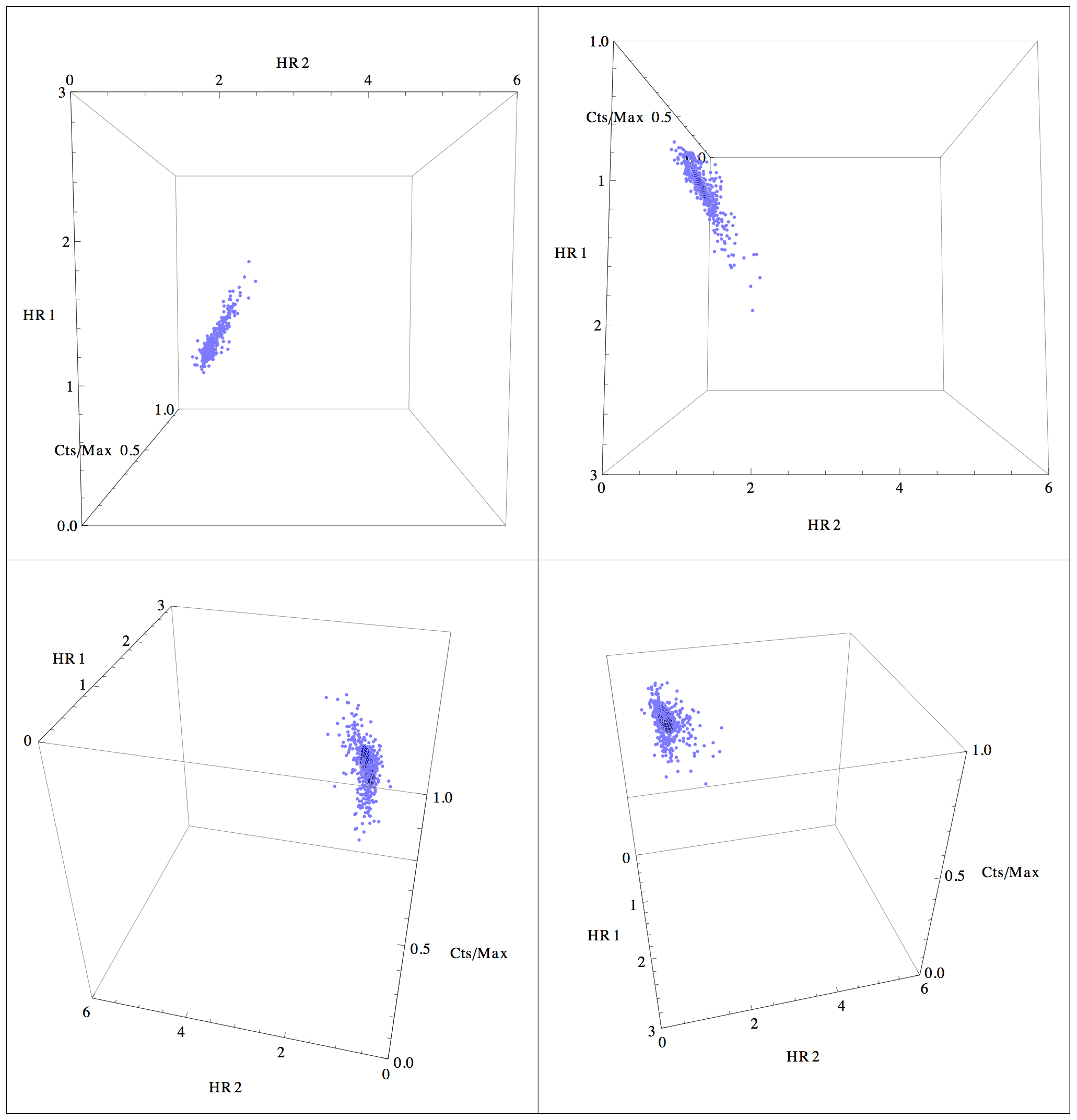
Figure 2: Four views of a CCI diagram of the last two years of the RXTE/ASM observations of the Crab. Only five sigma detections are plotted. The ellipsoid center and radii are significantly different from the first 13 years (see Table 2).

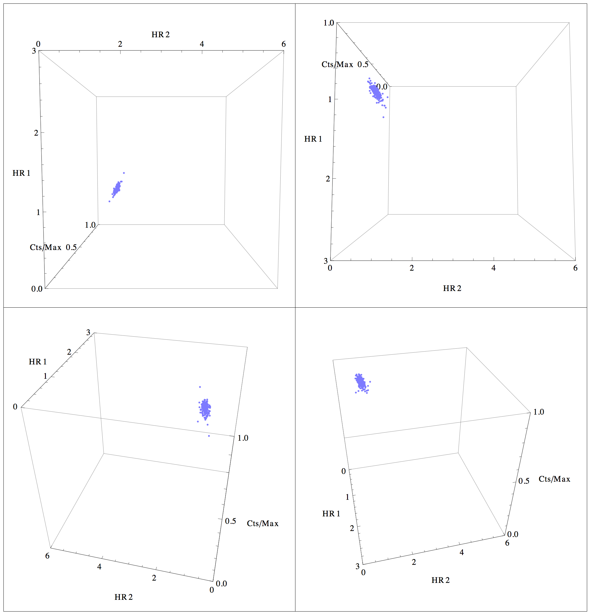
Figure 3: Four views of a CCI diagram of the 3rd and 4th years of the RXTE/ASM observations of the Crab. Only five sigma detections are plotted. The ellipsoid center and radii match that for any two-year interval within the first thirteen as well as for the first 13 years combined (see Table 2).

The background of the ASM/RXTE A band (1.3-3.0keV) can be subject to contamination by Solar UV radiation (A. Levine and R. Remillard, personal communication). This excess is flagged in the dwell-by-dwell data provided by the ASM team. By eliminating data points were this flag (column 13 of the dwell-by-dwell data file) exceeds 20 counts this problem can be avoided. There are six-eight dwells per day or well over 32,000 points for the 15 years; the number of points out of the dwells in which the flag exceeds 20 counts ranges from 150-300. We consider daily averages for our CCI diagrams and for the bright sources where there are over 4500 detections over 13 years, the possibility of 300 data points being corrupt is a less than 10% effect. For weak sources were there may be less than 1000 detected points this can be a significant effect. In this paper we restrict ourselves to strong sources (average counts greater than 2 ASM cts/sec): this removes from our sample 76 of the 122 XRBs for which we have extracted ASM light curves.

We are using one-day averages which for 13 years corresponds to about 4500 points for each source. We use the energy bands provided by the ASM/RXTE team (A:1.3-3.0 keV; B:3.0-5.0keV; C:5.0-12.2 keV) to define soft colour (HR1) as B/A and hard colour (HR2) as C/A. Summed counts (1.3-12.2keV) are shown on the intensity axis, scaled from 0-1 for each source. We only use points where the signal-to-noise of the ASM/RXTE in the summed intensity is greater than or equal to 5$\sigma$.

We have collected the sources in groups using the classification and nomenclature from Lvv00 and Lvv01 for NS systems and RM06 for BH systems (Table 1). We use the two hardness ratios and the summed intensity to construct 3-D “CCI” plots for each group. For each category of source we compute the centroid of all points as listed in Table 2. Using the Mathematica program EllipsoidQuantile we compute an ellipsoid around the centroid that contain 50% of all points while minimizing the volume of the ellipsoid.

Figures 4 and 5 shows CCI diagrams of all systems identified by RM06 as definitely containing BHs. We have separated systems with high-mass companions from systems with low-mass companions. The data of each object within a group are shown in different colours but the ellipsoid represents all objects of a given group. There is significant overlap between BH systems with low-mass and high-mass companions with the exception of GRS1915+105 (a rare microquasar that ejects material at superluminal velocities; Mirabel & Rodriguez 1994). We have separated out GRS1915+105 because it occupies a space that is disjoint from the other BH systems. We then considered systems identified by RM06 as BHCs. In Figure 6 we depict BHs with high-mass companions in blue, BHs with low-mass companions (with the exception of GRS1915+105) in cyan, BHCs (with the exception of J1630-472) in magenta. The ellipsoids and points for BHs and BHCs (with both low-mass and high-mass companions) overlap, whereas GRS1915+105 and J1630-472 clearly occupy a region distinct from the others.

Table 2: Centroids and radii

Source Type	Center	radius1 radius2 radius3
Fig1 Crab13	0.87, 0.95, 0.95	0.05,0.02,0.02
Fig2 Crablast2	0.94, 1.05, 0.86	0.25,0.06,0.06
Fig3 Crab2	0.87, 0.95, 0.95	0.05,0.02,0.02
Fig4 HMBHs	0.83, 0.87, 0.25	0.84,0.18,0.15
Fig5 LMBHs; no GRS1915+105	0.79,0.56,0.30	0.72,0.32,0.19
Fig5 GRS1915+105	1.96,2.60,0.28	0.86,0.25,0.16
Fig6 HMBHs	0.83,0.87,0.25	0.84,0.18,0.15
Fig6 LMBHs	0.79,0.56,0.30	0.72,0.32,0.19
Fig6 BHCs	0.95,0.68,0.22	0.41,0.23,0.13
Fig6 GRS1915+105 and 1630-472	2.09,2.75,0.28	1.13,0.32,0.17
Fig7 HMXB pulsars	1.45,3.21,0.34	1.74,0.30,0.22
Fig8 HMXB pulsars no outbursts	1.37,3.14,0.29	2.15,0.30,0.13
Fig8 HMXB pulsars with outbursts	1.52,3.28,0.39	1.26,0.33,0.22
Fig9 Bursters	0.95,1.02,0.39	0.44,0.24,0.15
Fig10 Atolls	1.31,1.61,0.51	0.89,0.20,0.19
Fig11 Z sources	1.27,1.55,0.49	0.77,0.12,0.10
Fig12 Classic BHs	0.82,0.80,0.26	0.87,0.21,0.19
Fig12 GRS1915-like BHs	2.09,2.75,0.28	1.13,0.32,0.17
Fig12 Pulsars	1.45,3.21,0.34	1.74,0.30,0.22
Fig12 Non-pulsing NS	1.31,1.63,0.53	0.84,0.17,0.15
Fig17 Bursters	0.95,1.02,0.39	0.44,0.24,0.15
Fig17 Atolls	1.31,1.61,0.51	0.89,0.20,0.19
Fig17 Z sources	1.27,1.55,0.49	0.77,0.12,0.10
Fig19 BHs with resolved jets	1.25,1.53,0.33	1.37,0.24,0.20
Fig19 Pulsars	1.45,3.21,0.34	1.74,0.30,0.22

Figure 7 shows systems where the NS is a pulsar. Only pulsars with high-mass companions are included as no pulsars with low-mass companions match our selection criterion. The sources that stick out from the bulk of the pulsars are ones that show X-ray outbursts. Figure 8 shows HMXB pulsars differentiated by those which do and do not show outbursts. The non-pulsing NS systems (bursters, atolls, and Z-sources) are plotted in Figures 9, 10, and 11.

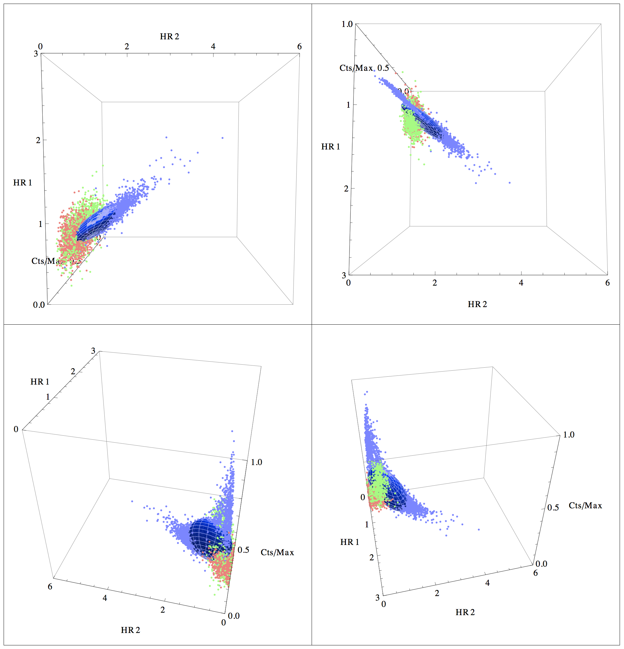
Figure 4: Four views of a CCI diagram of dynamically well-determined BHs with high mass companions as classified by RM06. Cyg X-1 (blue), LMC X-1 (red), LMC X-3 (green). A single ellipsoid (blue) has been fit to encompass 50% of all the points, centered on the centroid of all points. See Table 2 for values of the centroid.

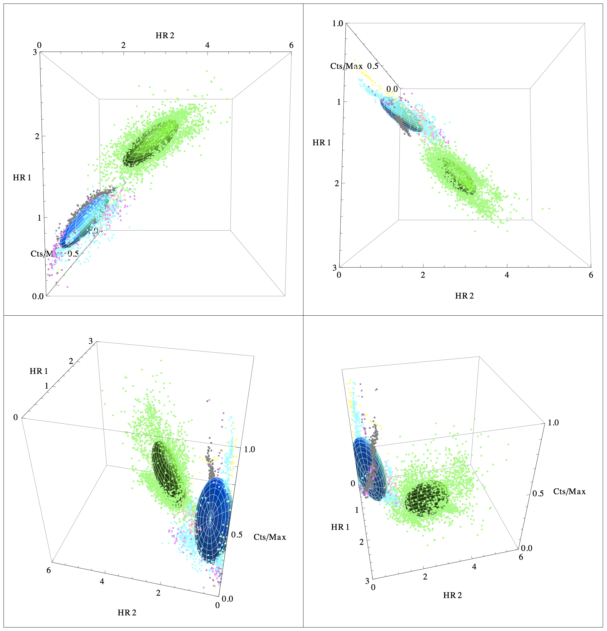
Figure 5: Four views of a CCI diagram of dynamically well-determined BHs with low-mass companions as listed in Table 1. 1118+480 (pink), 1550-564 (magenta), 1650-500 (yellow), 1655-40 (cyan), 1859+226 (purple), GRS1915+105 (green), GX339-4 (black). We note that GRS 1915+105 (green) occupies a space well separated from the rest of the LMXB BHs. Ellipsoids fitted to all LMBH excluding GRS1915+105 (cyan) and separately to GRS 1915+105 (green). See Table 2 for values of the centroids.

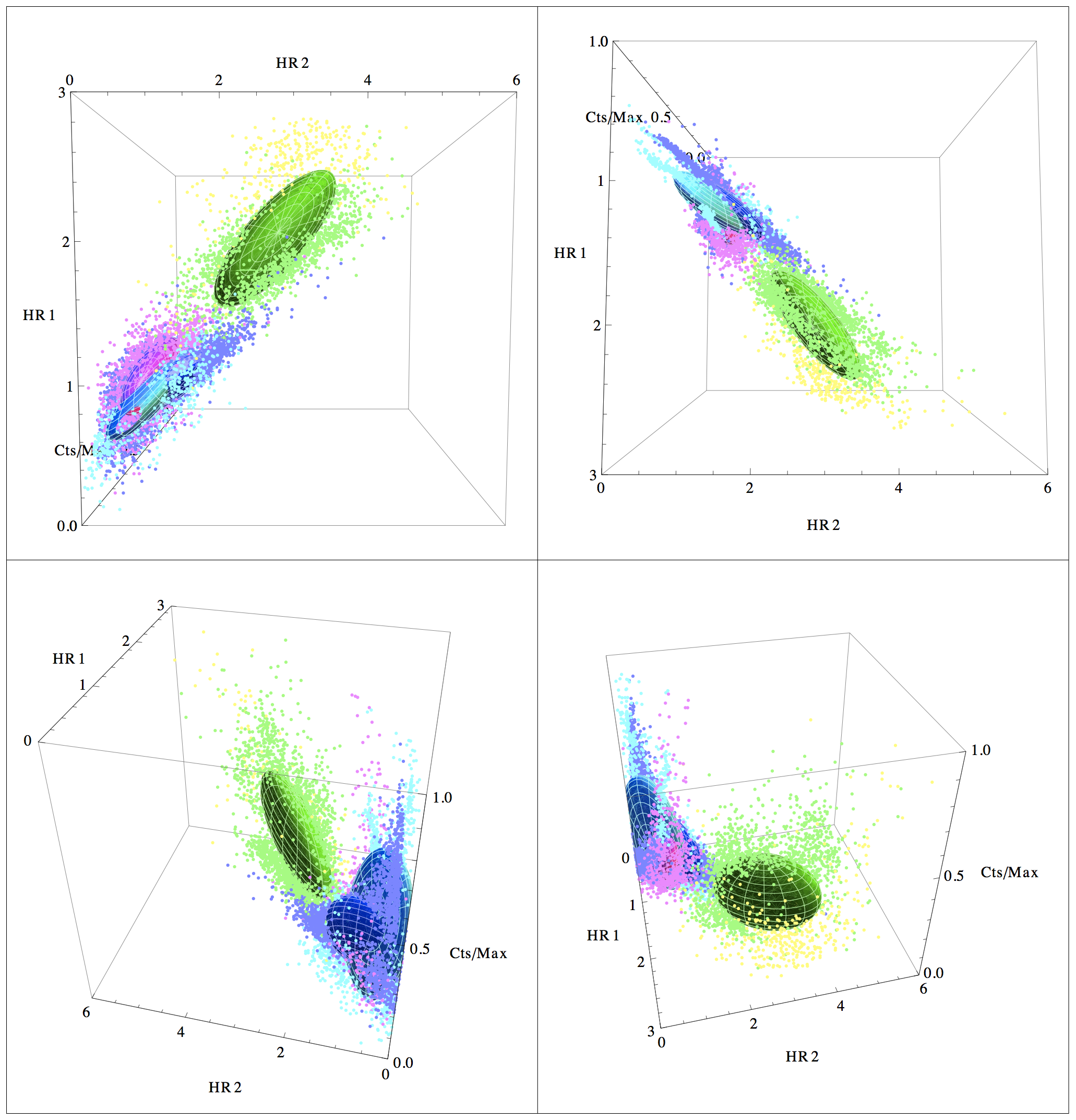
Figure 6: Four views of a CCI diagram of all dynamically well determined BHs with massive companions in blue, with low mass companions in cyan, all BHC candidate systems in magenta, GRS 1915+105 in green and J1630-475 in yellow (a single ellipsoid in green is fit to both these). See Table 2 for values of the centroids.

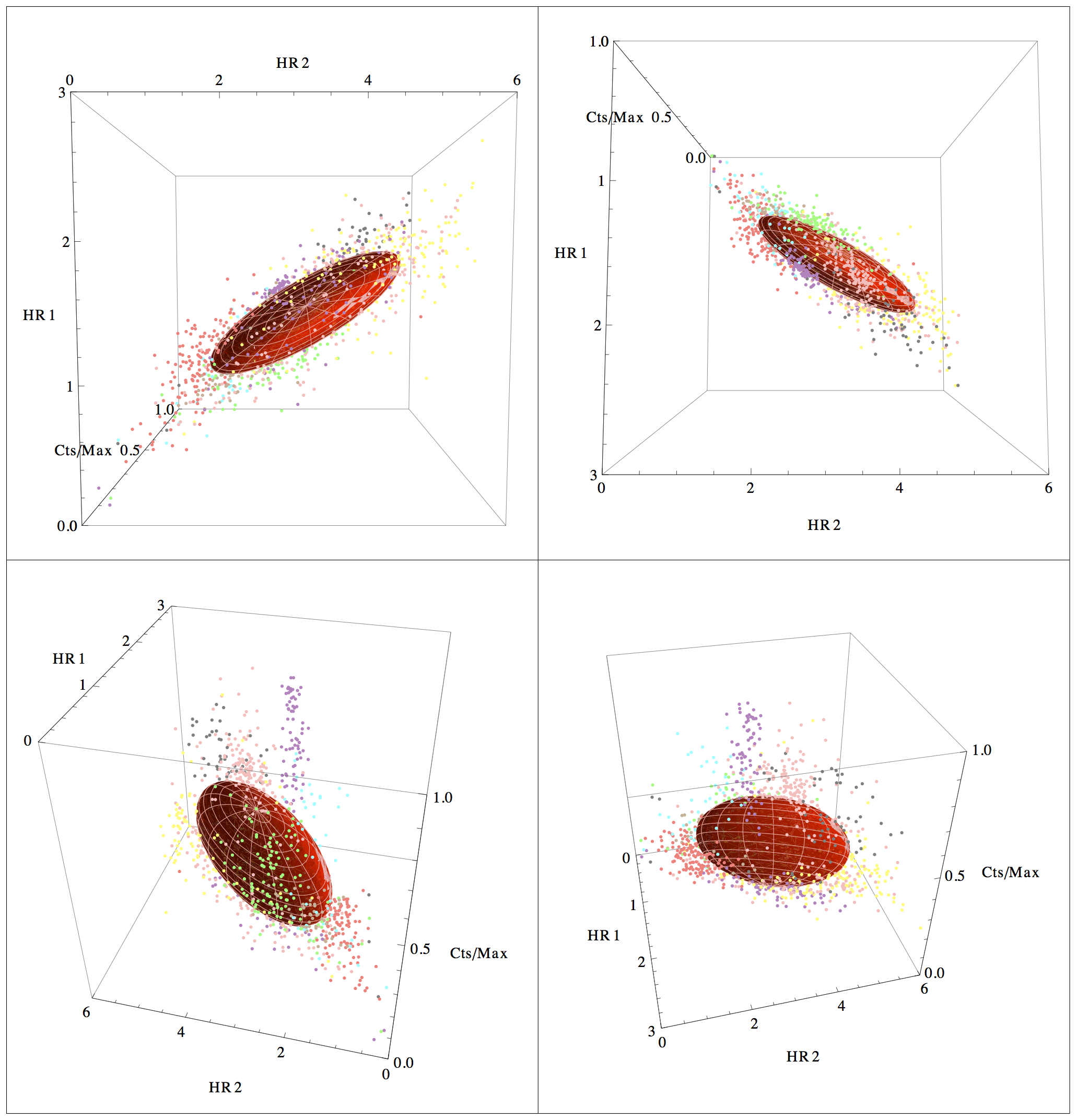
Figure 7: Four views of a CCI diagram of systems with high mass companions where the NS is a pulsar. Different colors represent different sources. The sources that stick up (1947+300 in cyan; 2030+375 in purple; Cen X-3 in pink; 1901+03 in red) are sources that have outburst states. A single 50% ellipsoid (red) is fitted to all points. See Table 2 for values of the centroid.

Figure 8: CCI diagrams of systems where the NS is a pulsar. 50% ellipsoids fitted to pulsars with outbursts (green) and all other pulsars (red). See Table 2 for values of the centroids.

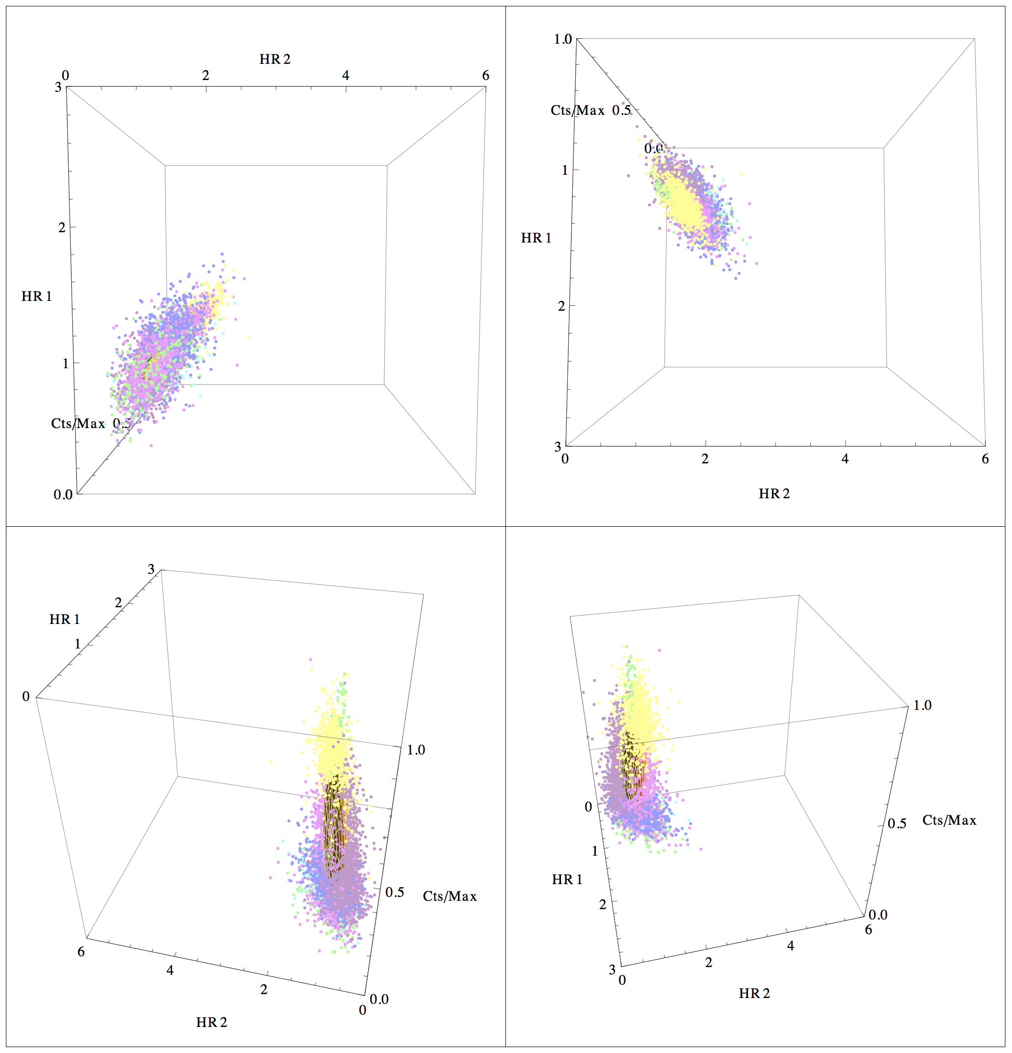
Figure 9: Different colours represent different sources. CCI of NS systems containing low-mass companions and identified as bursters. 50% ellipsoid fitted to all points (red). See Table 2 for values of the centroid.

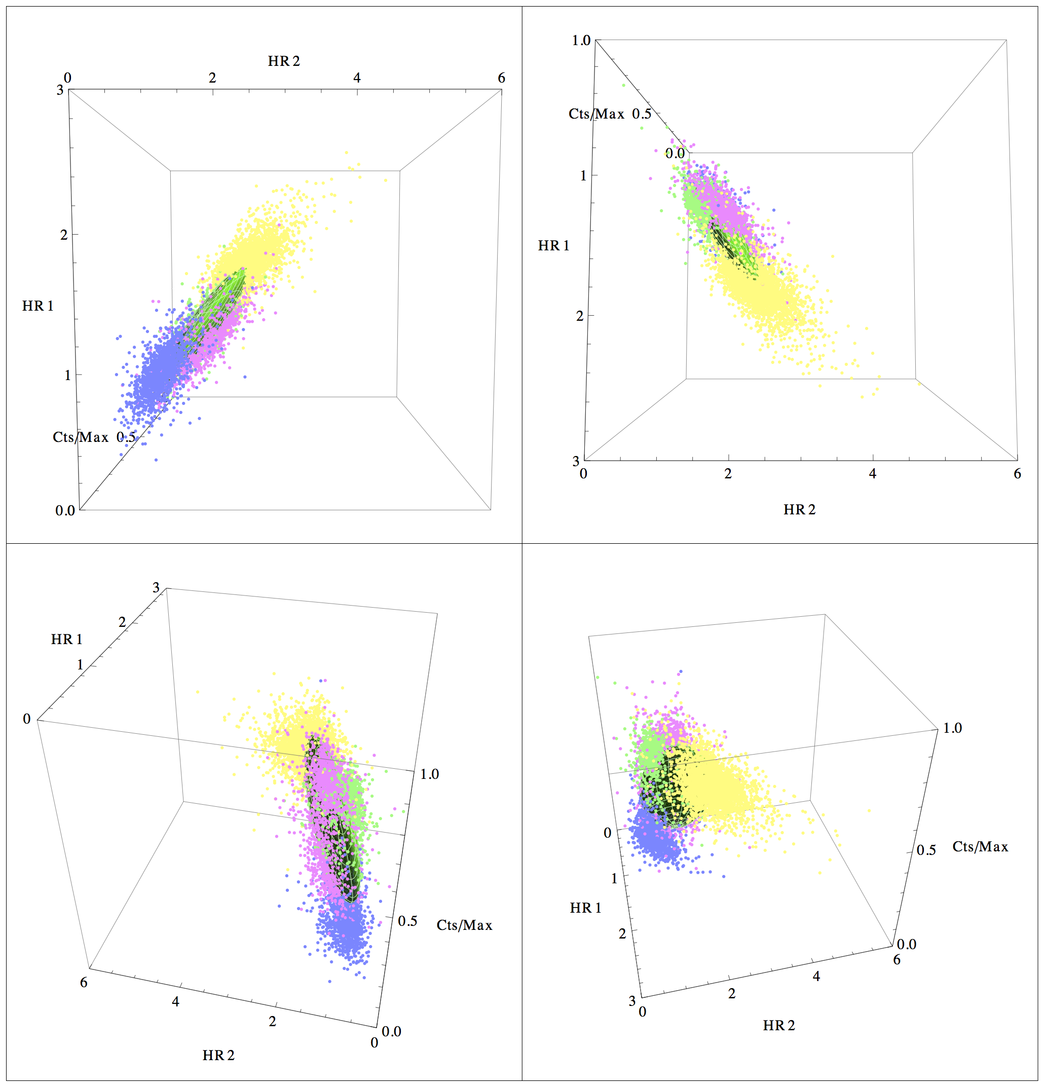
Figure 10: Different colours represent different sources. CCI of NS systems containing low-mass companions and identified as atoll sources. These overlap with bursters but go out to larger HR1, HR2 values. 50% ellipsoid fitted to all points (green). See Table 2 for values of the centroid.

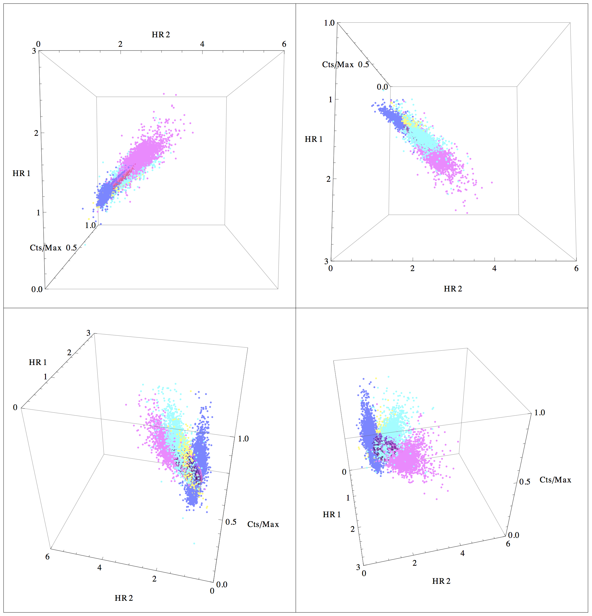
Figure 11: Different colours represent different sources. CCI of NS systems identified as Z sources. (Scox1 in yellow; Cyg X-2 in blue; GX17+2 in magenta; GX349+2 in cyan). 50% ellipsoid fitted to all points (magenta). See Table 2 for values of the centroid.

Figure 12: Four views of a CCI diagram of classic BHs binaries in blue; GRS1915-like BHs in green; pulsars in red, and non-pulsing NS systems in magenta. ellipsoid. It is clear that pulsars (red), classic BHs (blue), GRS1915-like BHs(green), and non-pulsing NS (magenta) are located in distinct regions. See Table 2 for values of the centroids.

Figure 12 shows classic and GRS1915-like BHs, and pulsing and non-pulsing NS systems on one plot. Classic BHs are depicted in blue, GRS1915+105 and J1630-475 are depicted in green, NS systems that pulse are depicted in red; and NS systems that do not pulse are depicted in magenta. Table 2 lists the centroid locations and length of each radius. While some of the 2D projections in Figure 12 may appear to show overlap between the different types, other projections of the same figure make it clear that there is in fact no overlap; not only for the ellipsoids but indeed for any of the points that extend beyond the ellipsoids.

We use the locations of classes of objects as pointed out above to classify the hitherto ambiguous systems empirically as listed in Table 3. It is immediately clear why some of these sources are difficult to classify: they overlap categories defined hitherto. For example, Cyg X-3 overlaps with GRS1915+105 which is classified by both RM06 and Massi & Bernado (2008; hereafter MB08) as a BH, but also spends a significant amount of its time in the region we associate sith pulsars (Fig. 13). Circinus X-1 classified by MB08 as a NS system does overlap with non-pulsing NS (Fig. 14). GX3+1 is clearly associated with non-pulsing NS (Fig. 15), and 1700-37 is clearly associated with pulsars (Fig. 16).

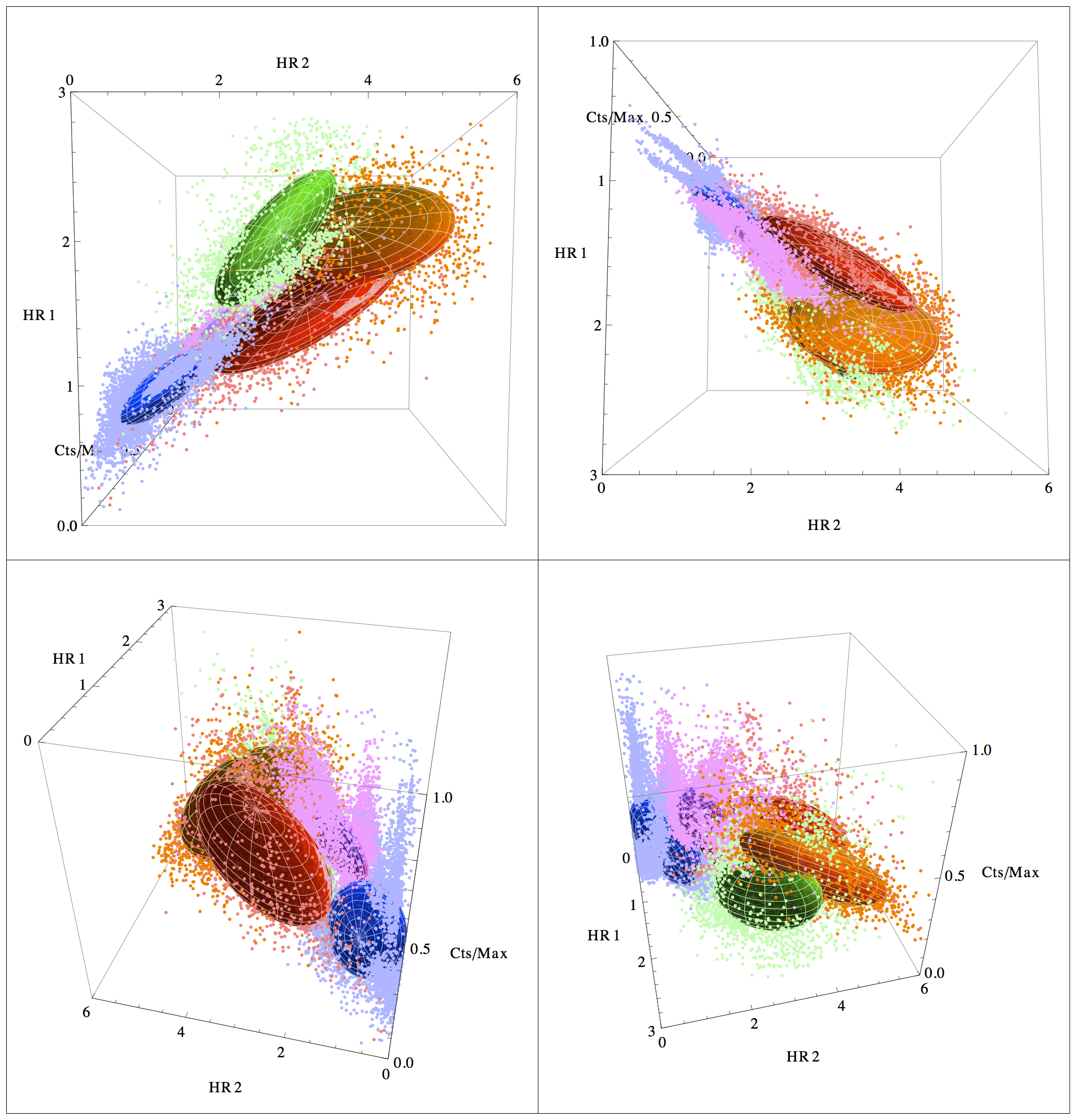
Figure 13: Comparison of unclassified sources Cyg X-3 (orange) with classic BH systems in blue; GRS1915-like BH systems in green; pulsars in red; and non-pulsing NS in magenta. Cyg X 3 (orange) overlaps with both GRS1915-like and pulsars.

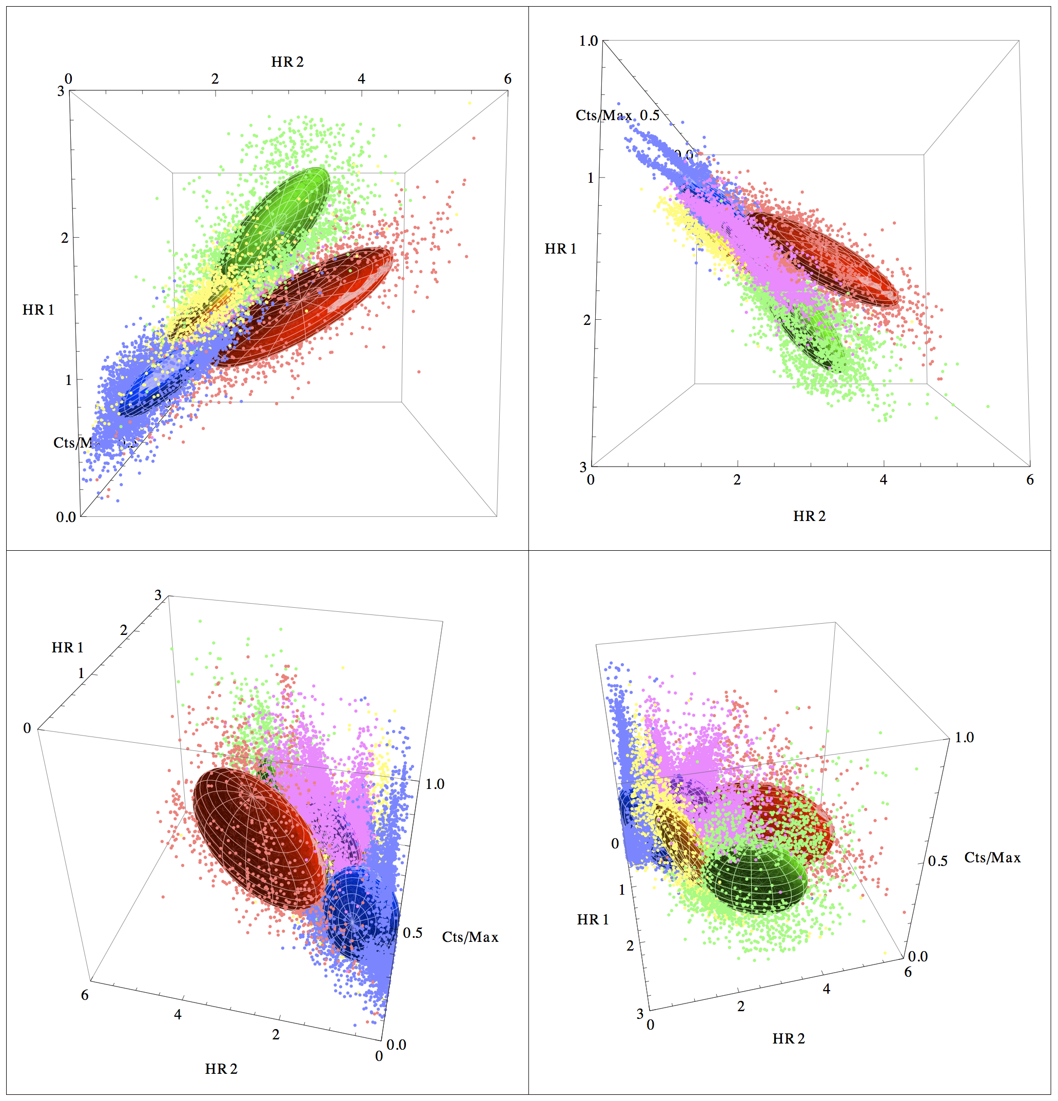
Figure 14: Comparison of unclassified sources Circ X-1 (yellow) with classic BH systems in blue; GRS1915-like BH systems in green; pulsars in red; and non-pulsing NS in magenta. Circ X-1 overlaps with non-pulsing NS.

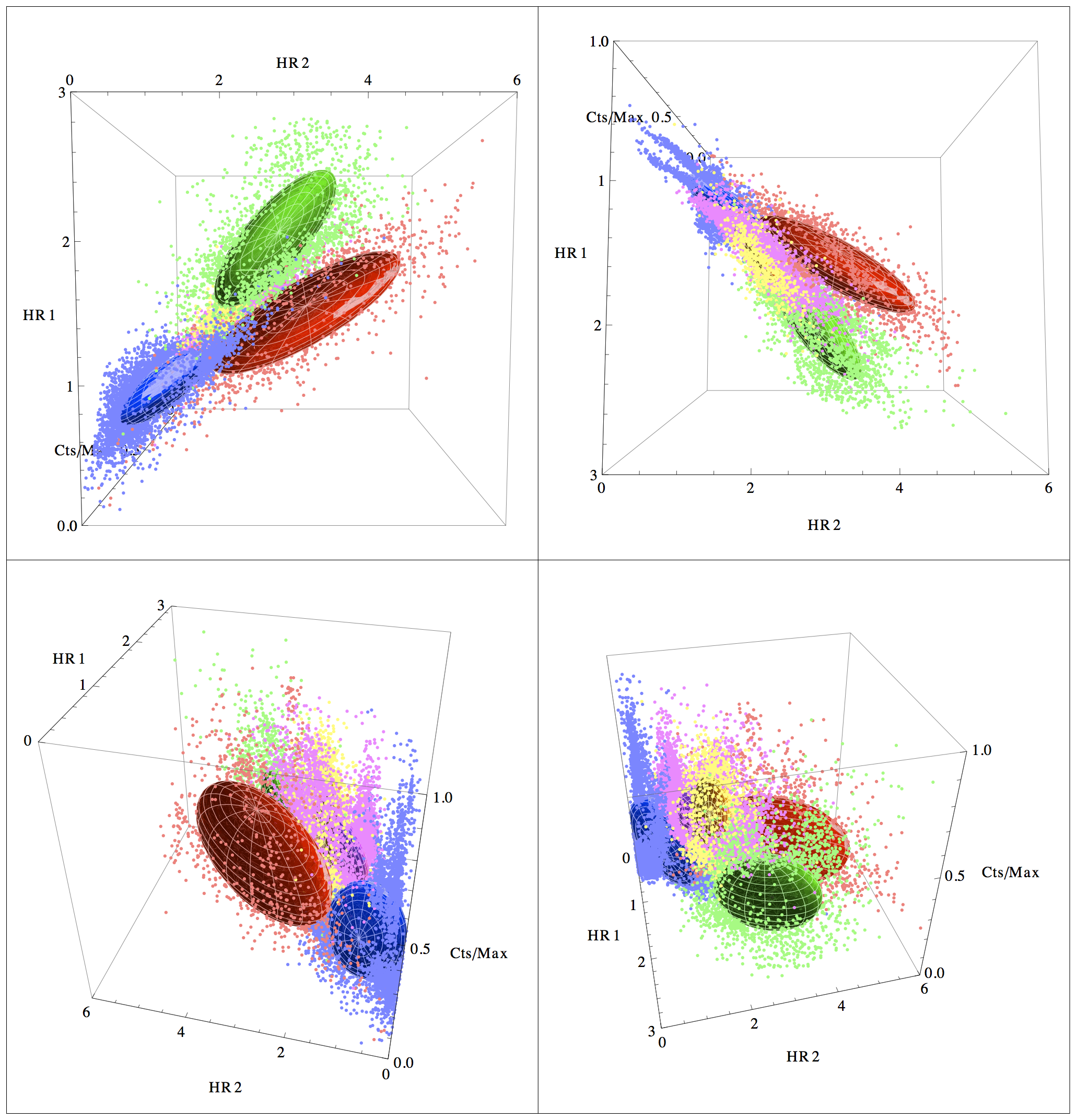
Figure 15: Comparison of unclassified sources GX 3+1 (yellow) with classic BH systems in blue; GRS1915-like BH systems in green; pulsars in red; and non-pulsing NS in magenta. GX 3+1 is consistent with being a Z-source.

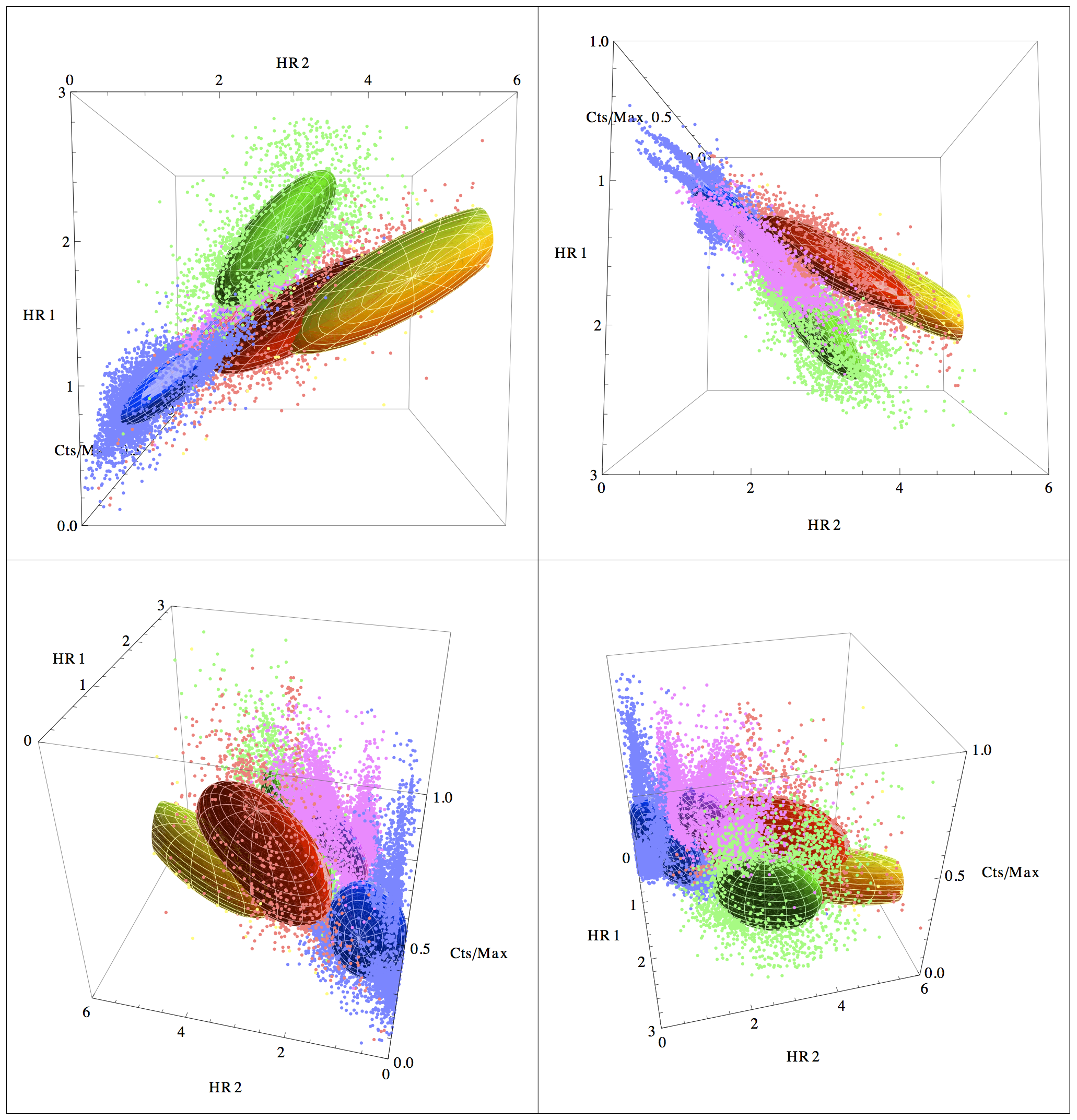
Figure 16: Comparison of unclassified source 1700-37 (yellow) with classic BH systems in blue; GRS1915-like BH systems in green; pulsars in red; and non-pulsing NS in magenta. 4U1700-37 is consistent with being a pulsar.

3 Interpreting CCI diagrams

The parameters that may be expected to influence X-ray emission (mass accretion rate, binary separation, orbit inclination, mass ratio, magnetic field strength, column density, etc.) are well established for many systems. Our CCI diagrams offer some clues as to how different parameters may relate to location in phase space: For example, Homan et al. (2010) conclude that the variety of behavior observed in atolls and Z-sources can be linked to mass-accretion rate increasing from atolls to Z-sources. MB08 have mass-accretion rate increasing from atolls to Z-sources (their Figure 3). Assuming this to be correct we plot bursters, atolls, and Z-source on one figure (Fig. 17) and find that mass-accretion rates increases on a diagonal from the corner with lowest values of HR1, HR2, and Intensity to the corner with high HRs and Intensity (Fig. 18). Note this implies that X-ray intensity within the ASM energy range is not a direct indication of mass accretion rate in agreement with our past work (Vrtilek et al.  1990, 1991, 1994).

Since the ASM is not very sensitive to NH we extracted the PCA data of sample sources, modeled the data, and adjusted the model for NH to see the effects. Adjusting for the nominal NH (6.2e22cm^-2) to GRS 1915+105 does place it closer to the other BH systems, but since the other BHs also move slightly there is still a separation between GRS1915+105 and all other BHs. But this is a model dependent result. The fact remains that the ASM raw data, uncorrected for NH, distinguishs four categories of sources: NS pulsing, NS non-pulsing, BH classical, and BH GRS1915-like. Detailed analysis of PCA data of individual sources using CCI is underway (Peris et al.  2012; Buchan et al.  2012; Cechura et al.  2012).

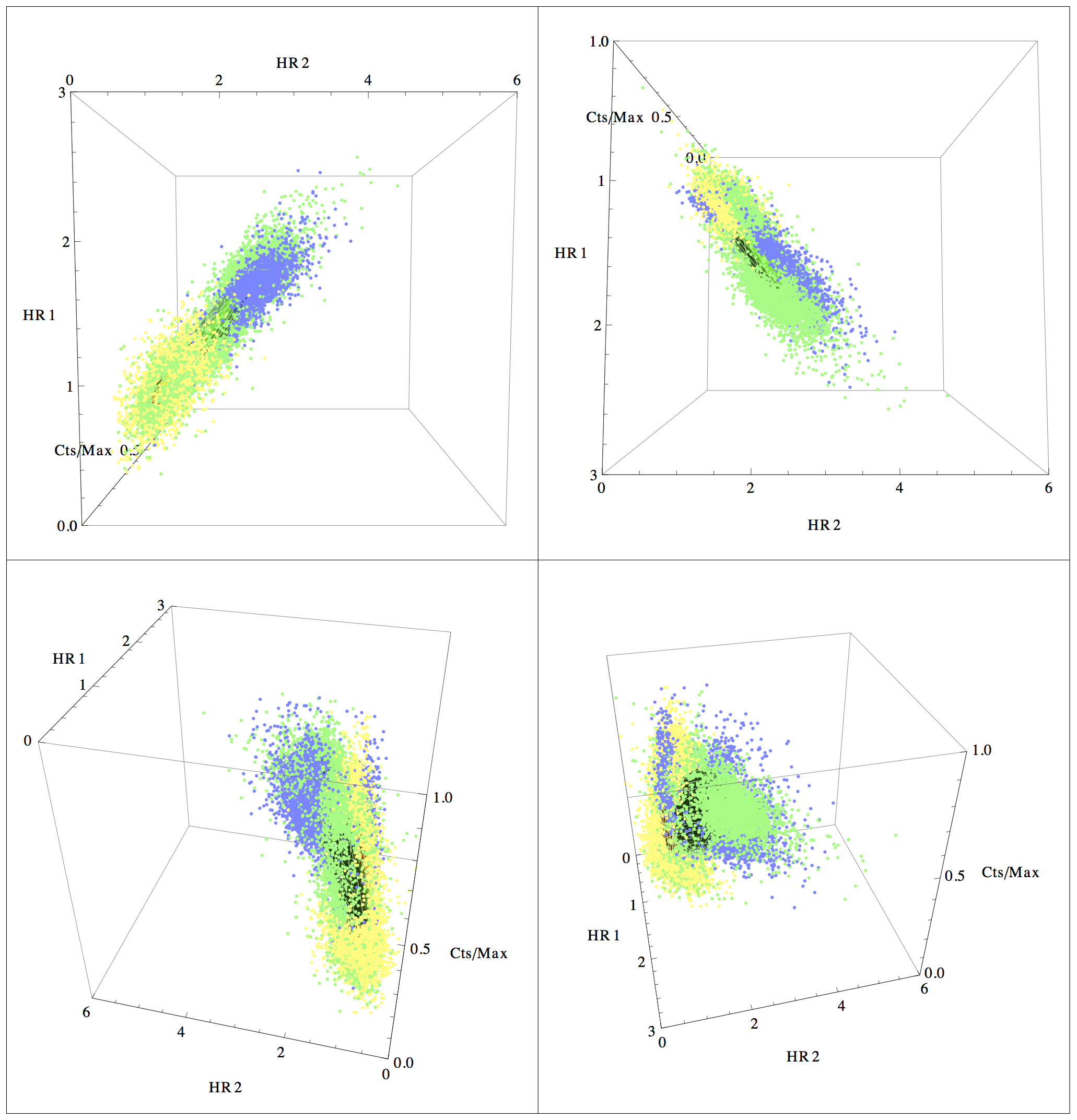
Figure 17: CCI diagram of bursters (yellow), atoll (green), and Z-sources (cyan). If we accept the premise that atolls and Z-sources are at higher mass accretion rates than Atolls with both higher than bursters than we can infer a direction for increasing mass accretion rate. Note that mass accretion rate does not have a simple relationship to the X-ray flux of the systems. 50% ellipsoids fitted to bursters (yellow); atolls (green), Z-sources (blue). See Table 2 for values of the centroids.

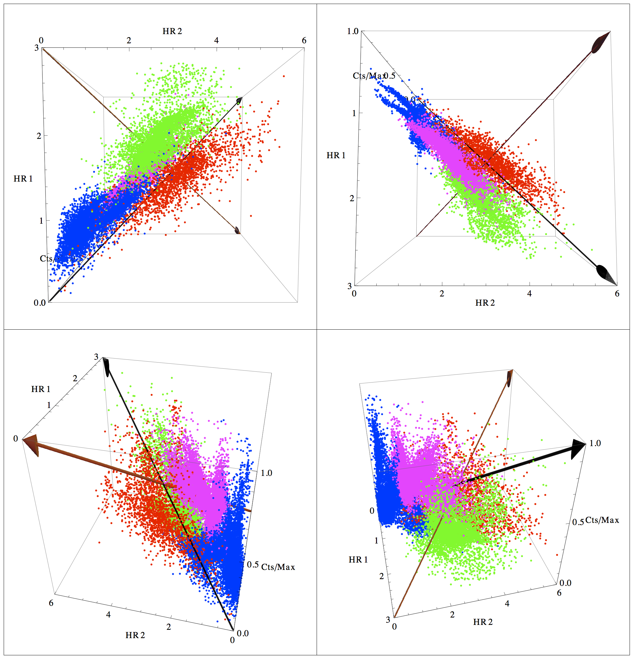
Figure 18: Classic BHs in blue, GRS1915-like BHs in green, pulsars in red, non-pulsing NS in magenta. Brown arrows shows direction of increasing magnetic field strength and black arrow shows direction of increasing mass accretion rate. The third axis may be a measure of the Alfven radius for NS and the ISCO for a BH as defined by Massi & Bernando (2008).

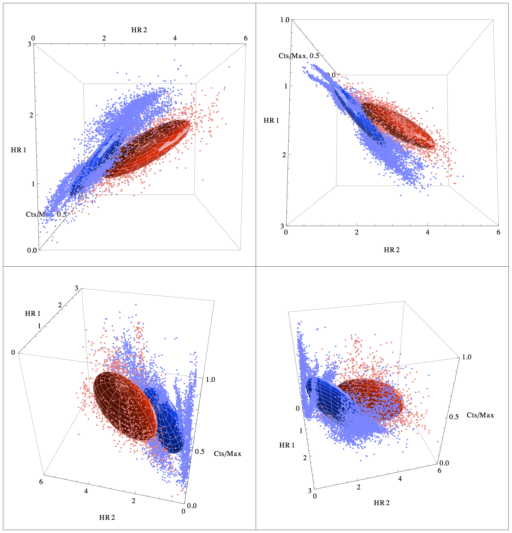
Figure 19: Four views of a CCI diagram with sources showing resolved jets in blue and pulsars in red. If we accept MB08 that pulsars cannot produce jets then we can define the region were pulsars exist as a jet exclusion region. 50% ellipsoids with all jet sources in blue and pulsars in red. See Table 2 for values of the centroids.

MB08 also suggest that pulsars, distinguished by very high magnetic fields, are clearly separated from all other classes (their Fig. 1). Migliari & Fender (2006; hereafter MF06) suggest a progression of source type associated with differing magnetic field strengths. Particularly interesting is that the distribution of the sources in our CCI diagram appear to follow the order delineated by MF06 for decreasing magnetic field strength. This order suggests that magnetic field strength in our CCI diagrams decreases diagonally from the corner with high HR2, low HR1, and low I towards the corner with low HR2, high HR1, and low I. So in the upper left we have sources with the strongest magnetic fields, the pulsars; going away from the pulsars towards the right we have first the Z sources and then BH systems.

Mass accretion rate and magnetic field strength represent two dimensions of our 3-D diagrams. MB08 agree with Homan et al. (2010) that mass accretion rate increases from atoll to Z sources. They agree with MF06 and Fender et al.  (1997) that X-ray pulsations and radio emission (taken as a measure of jet strength) are strongly anti-correlated. Following the work of MB08 we suggest that the third axis can be represented by the ratio of the Alfven radius to surface of the NS and the innermost stable circular orbit (ISCO) for BHs. For both BHs and NSs, we expect the inner accretion disc to be an important contributor to the spectrum. In the case of accreting NSs, we expect the inner radius will be related to the Alfven radius, which depends on the mass accretion rate and on the NS magnetic field. For the BHs, the emitting radius may scale with the general relativistic innermost stable circular orbit, which depends on the BH mass, spin, and spin sense (prograde or retrograde with the disc). The NS systems will have an additional source of emission as gas disrupted by the magnetic field near the Alfven radius is channeled onto the NS surface (for stronger magnetic fields, the channeling will direct the accretion onto a smaller area about the poles). Our CCI diagrams may be related to MB08’s physical model by a transformation of coordinates.

Table 3: Unclassified Objects

Object Name	Our classification
Circinus X-1	Non-pulsing neutron star
1700-37	Pulsar with massive companion
GX3+1	Non-pulsing neutron star
Cygnus X-3	Shares space with
	GRS1915-like and pulsars

3.1 Defining the Jet Locus?

MF06 suggest a progression of source type and activity correlated with the detection of jets. From most likely to least likely to show jets, these sources range from BH systems with no intrinsic magnetic fields, low-mass NS systems with weak magnetic fields at high accretion (Z type), low-mass NS systems with weak magnetic fields at low accretion (atoll type), and NS systems with strong magnetic fields (pulsars). In general, jet production is enhanced with mass accretion rate (as a means of expelling angular momentum) but it is inhibited by high magnetic fields on the surface of NSs or in BH accretion discs. MB08 quantified the progression suggested by MF06 by considering that in an accreting system magnetic fields lines can be bent only when the magnetic pressure is lower than the hydrodynamic pressure of the accreting material. The basic condition for jet formation is then that the location at which the magnetic pressure and plasma pressure balance (Alfven radius) is coincident with the NS surface or for a BH the innermost stable orbit.

MB08 list 15 XRB systems that have resolved jets and several additional systems with indirect evidence for compact jets in the form of a flat radio spectrum (seven of these are bright enough in the ASM for this study). The systems span a wide range of temporal and spectral morphologies, and in roughly half the systems the nature of the compact object is ambiguous.

Figure 19 shows systems containing both BHs and NSs identified by MB08 as having resolved radio jets as well as the pulsars which according to MB08 cannot produce jets. If we consider the progression of source type and activity correlated with the detection of jets suggested by Migliari & Fender (2006) we can imagine a curved plane that separates pulsing systems from the others. This plane cuts through several sources such as Cyg X-1 (blue), Sco X-1 (cyan), Cyg X-3 (magenta), and GRS 1915+105 (pink). We see that the progression is from upper left towards lower right: in the upper left are the pulsars with strong magnetic fields; going away from the pulsars toward the right we have first the atoll and Z sources (differentiated mainly by mass accretion rate) and then with the lowest magnetic fields the BH systems. This suggests that we can define a locus of our CCI space which contains systems that can form jets. The “jetline” as defined by Fender, Belloni, and Gallo (2005) is for us a curved plane that depends, not surprisingly, on a combination of magnetic field strength, Alfven radius or ISCO, and mass accretion rate. Since the ISCO depends on the spin parameter of the BH, this interpretation is also consistent with the recent connection made between BH spin period and jet power by Narayan & McClintock (2011). One of our ongoing projects is to define this “jet plane” on the CCI diagram (Boroson et al.  in preparation).

4 Summary and Future Work

We find that separate classes of XRBs fall into distinct regions on a 3-dimensional colour-colour-intensity (CCI) diagram. This provides a simple, model-independent method of distinguishing between systems that contain BHs or NSs, and between systems that contain pulsing and non-pulsing NSs. CCI diagrams may also help us to define the observable characteristics of systems that produce jets and localize a “jet plane” that separates systems that cannot produce jets from those that can.

A hint of the physics underlying this separation is provided by Massi & Bernado (2008) who characterize the systems in terms of their mass-accretion rate, their magnetic field strengths, and the location of the Alfven radius for NSs or the ISCO for BHs. Given that the loci of different classes of objects in CCI space is determined by intrinsic properties of the systems, using our prior knowledge of mass accretion rates and magnetic field strengths we can define the directions of increasing accretion rate and field strength. Other factors (e.g., binary separation, mass ratio) that may play roles are yet to be explored.

The ASM on RXTE has continuously monitored over 500 sources for the past 15 years. Only 200 of these sources are XRBs. The rest include a variety of bright X-ray emitters such as blazers, quasars, Seyfert galaxies, cataclysmic variables, and Wolf-rayet stars. It would be interesting to see if methods similar to those shown here can be used to distinguish between different classes of cataclysmic variables (novae, dwarf novae, polars, AM Can Ven) or galatic nuclei (blazers, quasars, Seyferts of types 1 and 2). Applying CCI techniques to a variety of active galaxies may provide another means of probing the microquasar/quasar connection.

Although the RXTE/ASM is no longer operating, MAXI (Monitor of ALL-sky X-ray Image; Matsuoka et al.  2009) operating on the Space Station measures the X-ray fluxes of over 1,000 X-ray sources (twice the number detected by the RXTE/ASM) over the energy range 1-30keV once every 96 minutes over the entire sky. Such data should allow us to extend our CCI analysis to many more sources, and enable us to study them out to significantly higher energies. The Chandra X-ray observatory has the demonstrated ability to detect XRBs in galaxies other than our own. M31 has been very well monitored by Chandra and may present an opportunity to apply CCI techniques to XRBs in an external galaxy.

5 References and Citations

Belloni, T., Klein-Wolt, M., Mendez, M., van der Klis, M., & van Paradijs, J. 2000, A&A, 355, 271.

Buchan, S., Peris, C., Boroson, B.S., & Vrtilek, S.D. 2012, (PCA observations of Cyg X-1), in preparation.

Cechura, J., Peris, C., McCollough, M., & Vrtilek, S.D. 2012, (PCA observations of Cyg X-3), in preparation.

Fender, R.P., Belloni, T., & Gallo, E. 2005, AP&SS, 300,1.

Fender, R.P. et al.  2004, Nature, 427, 222.

Hasinger, G., & van der Klis, M. 1989, A&A, 225, 79.

Homan J. et al.  2010, 719, 201.

Koljonen, K.I.I., Hannikainen, D.C., McCollough, M.L., Pooley, G.G., & Trushkin, S.A. 2010, MNRAS, 406, 307.

Levine,A.M. et al.  1996, ApJ, 469, 33.

Liu, Q.Z., van Paradijs, J., & van den Heuvel, E.P.J. 2001, A&A, 368, 1021. (Lvv01)

Liu, Q.Z., van Paradijs, J., & van den Heuvel, E.P.J. 2000, A&A Supplement Series, 147, 25. (Lvv00)

Matsuoka, M. et al.  2009, PASJ, 61, 999.

Massi, M, & Bernado, M.K. 2008, A&A,477,1. (MB08)

Migliari, S., & Fender, R.P., 2006, MNRAS, 366, 79.

Mirabel, I.F., & Rodriguez, L.F. 1994, Nature, 371, 46.

Narayan, R., & McClintock, JEM. 2011 (presented at a lunch talk at the CfA, paper is in press).

Peris, C., Boroson, B.S., & Vrtilek, S.D. 2012, (PCA observations of GRS 1915+105), in preparation.

Remillard, R., & McClintock, J. 2006, ARA&A, 44, 49. (RM06)

Vrtilek, S.D. et al.  1990, A&A, 235, 162.

Vrtilek, S.D. et al.  1991, ApJ, 376, 278.

Vrtilek, S.D. et al.  1994, ApJL, 436,9.

Wijnands, R. et al.  1998, ApJ, 504, L35.