A proposal for laser cooling antihydrogen atoms

Abstract

We present a scheme for laser cooling applicable for an extremely dilute sample of magnetically trapped antihydrogen atoms($\bar{\rm H}$). Exploiting and controlling the dynamical coupling between the $\bar{\rm H}$’s motional degrees of freedom in a magnetic trap, three-dimensional cooling can be achieved from Doppler cooling on one dimension using the $1s_{1/2}-2p_{3/2}$ transition. The lack of three-dimensional access to the trapped $\bar{\rm H}$ and the nearly separable nature of the trapping potential leads to difficulties in cooling. Using realistic models for the spatial variation of the magnetic fields, we find that it should be possible to cool the $\bar{\rm H}$’s to $\sim 20$ mK even with these constraints.

I Introduction

Two years ago the ALPHA collaboration demonstrated trapping of $\bar{\rm H}$ atoms.ALPHA1 This result was quickly followed by an improvement in the trapping rate and a measurement of the lifetime of $\bar{\rm H}$’s in the trap; $\bar{\rm H}$ were shown to be trapped for longer than 15 minutes.ALPHA2 The long time that the $\bar{\rm H}$’s remain trapped is important because it opens the possibilities to performing measurements that might require several minutes. ALPHA was able to use the long trapping time to perform the first measurement of resonant transitions between $\bar{\rm H}$ bound states.ALPHA3 Recently, the ATRAP collaboration have also published results where they claim to have trapped $\bar{\rm H}$.ATRAP

One of the difficulties in measuring the spectroscopic transitions in $\bar{\rm H}$ is that the trapped $\bar{\rm H}$’s are currently at relatively high energies which will lead to line broadening from the Doppler effect and from Zeeman shifts. To date, the trapped $\bar{\rm H}$ are formed using three body recombinationGO ; RH when an antiproton ($\bar{\rm p}$) is inside of a positron (e⁺) plasma. Because three body recombination is a relatively slow process at the densities and temperatures in the $\bar{\rm H}$ traps compared to collisional slowingHCT ; FR , it is estimated that the $\bar{\rm p}$ will approximately be in thermal equilibrium with the e⁺ plasma before recombination occurs. Typical temperatures reported for the e⁺ plasma have been a couple 10’s of Kelvin. Since the magnetic trap depth for $\bar{\rm H}$ is only $\sim 1/2$ K, the $\bar{\rm H}$’s have an energy distribution that extends from 0 to the trap depth. This was measured in Ref. ALPHA2 where the distribution of $\bar{\rm H}$ annihilations as a function of time or as a function of axial position of the trap matched that for the expected $\bar{\rm H}$ energy distribution.

Currently, trapped $\bar{\rm H}$ atoms have energies up to $\sim 500$ mK, and occupy a large volume of order (2 cm)${}^{2}\;\times$ 30 cm. They are in a strongly non-uniform magnetic field, varying by order 1 TALPHA1 , from the center to the walls of the trap. While a number of important experiments have been performed or planned in such a trap, laser cooling of $\bar{\rm H}$, if achieved, will provide a major experimental advantage.

Laser cooling will create a cold, and spatially localized sample of antimatter atoms. Localized atoms will be much less susceptible to the Zeeman effect, currently a dominant limitation for microwave spectroscopyALPHA3 , and one of the limitations for future laser spectroscopyHZ . The lower velocities of cooled atoms will reduce 2nd order Doppler broadening for 1s-2s two photon spectroscopy. Importantly, laser cooling will greatly increase the sensitivity for observing gravitational interaction of antimatter (see e.g. Ref. MCF ).

Only one experiment so far has reported laser cooling of atomic hydrogen, nearly 20 years agoSWL . In that experiment, $\sim 10^{11}$ atomic hydrogen at 80 mK, pre-cooled via evaporative cooling, was laser cooled to 8 mK in 15 min. While it is theoretically possible to cool the $\bar{\rm H}$’s in a similar manner, $\bar{\rm H}$ laser cooling presents considerable experimental challenge for several reasons: (1) generation of coherent radiation at 121.6 nm remains technologically difficult, due to the lack of convenient lasers and nonlinear crystals at these wavelengths. (2) experimental requirements for $\bar{\rm H}$ trapping allow only limited optical access to the trapped atoms. (3) because of the very low densities of $\bar{\rm H}$, three-dimensional cooling assisted by collisionally mixing the degrees of freedom (needed for laser cooling of atomic hydrogenSWL ) is prohibitive. (4) because of the large Zeeman effects, only a small portion of the trapped atoms resonantly interact with photons.

Several proposals exist for overcoming some of these challengesZG ; DK ; WBP , but none has been experimentally realized. Reference HMP demonstrated laser cooling of magnetically trapped Na atoms to $\sim 2$ mK using a one-dimensional optical molasses. This experiment showed that it is possible to obtain substantial cooling even with the severe restriction to one laser. In this paper, we will investigate whether this simpler scheme for laser cooling of $\bar{\rm H}$ will work, and show, via detailed numerical calculations for ALPHA-type apparatus, that three-dimension cooling to $\sim 20$ mK should be possible within realistic experimental and technological constraints.

In our scheme, the Doppler coolingMS will drive the $1s_{1/2}-2p_{3/2}$ transition with the light being linearly polarized perpendicular to the quantization axis in order to drive the $m=1/2$ to $m=3/2$ transition. By driving this transition, the light scattering does not lead to a spin-flip which would cause the atom to be ejected from the trapSWL .

While a powerful narrow-line cw Lyman-alpha laser could eventually offer advantages in laser cooling, development of such sources remain considerable challengeEWH ; SKM . In this work, we consider the use of a modern pulsed Lyman-alpha sourceTM , whose time-averaged (as well as instantaneous) power is much greater than cw. Because Lyman-alpha generation requires highly non-linear processes, a pulsed scheme offers overall better cooling efficiencies, as long as the transition per pulse is not saturated.

A key feature of the present scheme is the exploitation, and the control of the dynamical coupling between the $z$- and $xy$-degrees of freedom. This will allow three dimensional cooling in an ALPHA-type apparatus in which optical access is currently limited to one dimension due to constraints for efficient magnetic trapping as well as high sensitivity particle detection.MCF

While the trapping fields are clearly non-separable in $x,y,z$ near the walls of the trap, this is not true near the trap center. The effective potential energy for the $\bar{\rm H}$’s near the trap center approximately has the form $V_{1}(z)+V_{2}(r)$ where $r=\sqrt{x^{2}+y^{2}}$ and $z$ is along the trap axis. Since the light is nearly parallel to the trap axis, this nearly separable potential allows fast cooling of the $z$-motion but can lead to heating in the $xy$-coordinates.

However, there is some small coupling between the $z$-motion and the $xy$-motions. This coupling is the conduit through which we can achieve cooling in all directions. We enhance this coupling by the use of non-harmonic magnetic fields in both $xy$- and $z$- directions, in contrast to standard harmonic magnetic traps. In the $xy$-directions, the effective potential is given by $\sim r^{6}$, while in the $z$-direction we use total of five solenoidal coils to produce the nonlinearity. Three dimensional cooling is possible when the time between photon scatterings is comparable to or longer than the mixing time between all of the degrees of freedom. This leads to non-trivial behavior of the final temperature on the laser power.

In this paper, we will present results on many of the important aspects for laser cooling in this constrained geometry. We have investigated the time dependence of the cooling, the energy distribution versus detuning, the optimum detuning, etc. In the results section, we give physical reasons for the difficulties in trying to laser cool $\bar{\rm H}$.

II Numerical Method

The basic physical situation is that the $\bar{\rm H}$’s classically move through the trap. When the laser is on and the atom is within the waist of the field, the atom can scatter a photon. The atom receives two momentum kicks for each time a photon is scattered: when the photon is absorbed the atom is kicked in the $z$-direction and when the photon is emitted the atom is kicked in a random direction. The size of each momentum kick is $h/\lambda\simeq 5.45\times 10^{-27}$kg m/s. This corresponds to a velocity kick to an $\bar{\rm H}$ of $\sim 3.3$ m/s. The $\bar{\rm H}$’s cool when the total momentum kick is opposite the momentum of the $\bar{\rm H}$. In this section, we describe the computational techniques we used to model this process.

II.1 Classical motion

The $\bar{\rm H}$’s move through a magnetic trap where their de Broglie wavelength is much smaller than the trap dimensions. This means we can solve for their motion using classical forces. The potential energy for the center of mass motion is equal to $U=-\vec{\mu}\cdot\vec{B}$ where $\mu$ is the magnetic moment of the $\bar{\rm H}$ in the $1s$ state; $\mu$ is approximately the magnetic moment of the e⁺. Since the precession frequency is much higher than other motional frequency scales, the angle between $\vec{\mu}$ and $\vec{B}$ is an adiabatic invariant. This means the orientation of the positron spin with respect to the magnetic field does not change. Thus, the trapped $\bar{\rm H}$’s experience a potential $U=\mu B$ where the $\mu$ is the magnitude of the magnetic moment and $B=|\vec{B}|$.

To compute the force, we need to obtain

$$\vec{F}=-\vec{\nabla}U=-\mu\vec{\nabla}B$$ (1)

where we need to compute the gradient of the magnitude of the magnetic field. Because the magnetic field is a very complicated function of the coordinates, we computed it numerically using a central two point difference:

$$F_{x}=-[U(x+dx/2,y,z)-U(x-dx/2,y,z)]/dx$$ (2)

and similar operations for $F_{y}$ and $F_{z}$. We used $dx=dy=dz=R\times 10^{-5}$ where $R$ is the radius of the trap $\sim 2.2$ cm. Although this seems a crude approximation, the error is actually quite small. The error term in the gradient is $(dx^{2}/48)U^{\prime\prime\prime}$; since $U^{\prime\prime\prime}\sim U^{\prime}/R^{2}$, this approximation gives a relative error of $\sim 10^{-11}$ which is comparable to the round-off error in this approximation.

One of the big problems in the calculation is that we need to solve for the $\bar{\rm H}$ motion for 100’s of seconds. We need to be careful that there is no energy drift in the calculation which would either give an unphysical cooling (which would lead to overly optimistic results) or an unphysical heating (which would lead to a suppression of the laser cooling). We found that the adaptive step-size Runge-Kutta algorithm that worked well for the shorter times needed to model the results in Refs. ALPHA1 ; ALPHA2 ; ALPHA3 ; ALPHA4 was not accurate enough for the present calculations unless we used very small time steps. We found that the fourth order symplectic integratorEFR ; HYo ; JCR worked well for this calculation. As is usual with symplectic integrators, we found that the energy varied during the calculation but the variation remained within a small energy region; thus, there was no energy drift at long times. We used a time step of 20 $\mu$s in our calculations.

As with our previous investigations, we launched the $\bar{\rm H}$’s within an ellipsoidal region with a flat spatial distribution. The ellipsoid had a scale length of 0.8 mm in the $xy$-coordinates and scale length of 8 mm in the $z$-coordinate. The initial velocity distribution was chosen from a thermal distribution with a temperature $\sim 50$ K except where explicitly stated otherwise. Since the trap depth is only $\sim 0.5$ K, our effective velocity distribution is flat in velocity space within a sphere delimited by the trap depth. Before turning on the laser pulses, we had the $\bar{\rm H}$’s move through the trap for 2 s plus a random time between 0 and 0.2 s to model the fact that there is a delay between the $\bar{\rm H}$ formation and manipulations done to them. This time delay allows the $\bar{\rm H}$ to reach somewhat random regions of phase space.

The trapping field is generated using an octupole field to provide radial confinement and mirror coils to provide axial confinement. We used the approximations in Appendix A of Ref. ALPHA4 for the fields from mirror coils and the octupole field. Instead of two mirror coils, we used 5 coils in order to mimic the more complicated magnetic geometry in the ALPHA-II trap. All coils are approximated as two loops with the approximate vector potential of Eq. (A.2) of Ref. ALPHA4 . All coils have a radius $a=45.238$ mm and $\lambda=0.90230$. The two end mirror coils have a loop separation of 8.425 mm and a center-to-center separation of 274 mm. The other 3 coils are equally spaced between the two end mirror coils. All 3 of these coils have a loop separation of 8.083 mm.

The purpose of the extra 3 coils is to provide a flatter magnetic field in the center of the trap. Without the extra coils, the B-field near the center of the trap is quadratic in $z-z_{mid}$. One coil at the center can cancel the quadratic dependence and give a B-field that has a quartic dependence. The coils at the 1/4 and 3/4 position together with the middle coil can cancel both the quadratic and quartic dependence. This will give a B-field proportional to $(z-z_{mid})^{6}$ near the center of the trap.

We use 3 different currents through these 5 coils: the end mirror coils have the same current and the coils at the 1/4 and 3/4 position have the same current. In most of the calculations, we chose currents to give the flattest possible B-field. For our coil parameters, this is achieved with 606 A in the end coils, -57.8 A in the coils at the 1/4 and 3/4 position, and -2.5 A in the middle coil. We did perform calculations with somewhat different currents; these calculations will be discussed in the Results section.

Figure 1 shows a slice through the magnetic field given in terms of the Zeeman shift in mK units. The nearly rectangular nature of the contours highlight the nearly separable nature of the potential energy experienced by the $\bar{\rm H}$’s at low energy.

II.2 Light scattering

To perform realistic calculations, we need to use parameters for the 121.6 nm light that are within current technical capabilities. We used parameters suggested to us by T. Momose.TM We assumed a laser with a 10 Hz repetition rate. We assumed the laser pulse would be on for a short time, $\sim 10$ ns; this time is so short that we consider both the absorption and re-emission to happen instantaneously. We used a laser linewidth (FWHM) of 100 MHz. The total energy in one laser pulse was taken to be 0.1 $\mu$J. Calculations were mostly performed with the laser propagating exactly along the $z$-axis and the laser was assumed to be linearly polarized with a waist radius of 10 mm. Some calculations were performed at different directions for laser propagation and will be discussed in the Results section.

We used a semiclassical treatment of laser cooling to model the interaction between $\bar{\rm H}$’s and the laser field. If the atom is within the laser waist, the probability for absorbing a photon during one of the laser pulses is

$$P=\frac{3}{8}\frac{c^{2}}{hf^{3}}\Gamma_{sp}\frac{(\Gamma_{sp}+\Gamma_{las})/(2\pi)}{\Delta\omega^{2}+[(\Gamma_{sp}+\Gamma_{las})/2]^{2}}\frac{E_{las}}{\pi w^{2}}$$ (3)

where $\Gamma_{sp}$ is the spontaneous decay rate of the $2p$ state ($2\pi 99.7$ MHz $=626$ MHz), $\Gamma_{las}$ is the laser line width ($2\pi\;100$ MHz, FWHM), $\Delta\omega$ is the detuning of the laser (combination of laser detuning, Doppler shift, and Zeeman shift), $E_{las}$ is the energy in the laser pulse, and $w$ is the radius of the laser waist. We will measure the laser detuning from the transition at the minimum B-field, $B_{min}$, and denote it by $\Delta\omega_{0}$. The Doppler shift is $-\omega_{1s,2p}v_{z}/c$ where $v_{z}$ is the z-component of the $\bar{\rm H}$ velocity and $\omega_{1s,2p}=(E_{2p}-E_{1s})/\hbar$ is the transition frequency between the $1s$ and $2p$ states. The Zeeman shift is $-\mu_{B}(B-B_{min})/\hbar$ where $\mu_{B}$ is the Bohr magneton because the $m=3/2$ upper state shifts more strongly in the magnetic field than the $m=1/2$ ground state. Thus, the detuning in Eq. (3) is given by

$$\Delta\omega=\Delta\omega_{0}-\omega_{1s,2p}v_{z}/c-\mu_{B}(B-B_{min})/\hbar$$ (4)

where $B$ is evaluated at the position of the $\bar{\rm H}$.

The algorithm to incorporate the photon scattering worked in the following way. We stepped the $\bar{\rm H}$ using the symplectic time step of 20 $\mu$s. A laser pulse is sent through the trap every 5000^th step. Nothing happens if the $\bar{\rm H}$ is outside the waist. If the $\bar{\rm H}$ is within the waist, we use a random number generator and compare to the probability to scatter a photon in Eq. (3). If the random number is smaller than this value, then the atom’s velocity is modified by the two kicks. The two kicks give a change in velocity: $\vec{v}\rightarrow\vec{v}+\hat{z}\Delta v+\hat{\nu}\Delta v$ where $\Delta v$ ($\simeq 3.3$ m/s) is the photon momentum divided by the $\bar{\rm H}$ mass and the random direction $\hat{\nu}$ is opposite the direction of the photon emission. The vector $\hat{\nu}$ is randomly chosen from the photon emission distribution for a circularly polarized state.

The cooling discussed below should be compared to the cooling in a three-dimensional (B-field free) optical molasses. The lowest average atom energy is when the laser detuning is set to $\Delta\omega_{0}=-(\Gamma_{sp}+\Gamma_{las})/2$ and gives an average energy of $E_{av}=3\hbar(\Gamma_{sp}+\Gamma_{las})/4$. For our laser parameters, the $E_{av}/k_{B}\simeq 7.2$ mK. The recoil energy is $E_{rec}/k_{B}=M\Delta v^{2}/(2k_{B})\simeq 0.64$ mK.

III Results

There are two important issues that need to be addressed: what is the best laser detuning and how long is needed to get substantial cooling. The optimum detuning depends on the laser power for this system because the laser only directly cools one direction which is nearly separable from the other two directions. For our laser parameters, we found that the detuning should be substantially shifted from the B-field free optical molasses. We found optimal cooling with the field free detuning when we performed calculations where the laser could cross the trap at a large angle so that there was substantial components in $z$- and $x$- or $y$-directions, but this will not be an option for the ALPHA experiment.

We can obtain an overview of the cooling through the time dependence of the temperature of the trapped $\bar{\rm H}$’s. Figure 2 shows the average energy of the laser cooled $\bar{\rm H}$’s as a function of the time that the laser is on. The atoms start with the distribution that is trapped from a 54 K $\bar{\rm H}$ distribution. The figure shows the results for several possible detunings of the laser. The solid, dotted, dashed, and dot-dash lines are for the trapping potential in Fig. 1. Discussed below, the dash-dot-dot-dot line is the best cooling that could be obtained when the trapping potential is only from the two mirror coils at $\pm 137$ mm. The value of the detunings are given in terms of the optimal value of $-(\Gamma_{las}+\Gamma_{sp})/2$ when $B=0$.

This figure shows that the most rapid cooling occurs at early times and the cooling rate has substantially slowed near the final times. A pessimistic interpretation is that this suggests it will take quite a long time to reach the asymptotic temperature. As will be seen in the figures below, a large fraction of the $\bar{\rm H}$’s seem to cool to energies under 100 mK within 200 s while some $\bar{\rm H}$’s seem to remain at a few 100 mK. The hotter atoms have substantially fewer photon scatterings compared to the colder atoms. Thus, the colder atoms will interact more with a laser in a spectroscopy experiment which will lead to a somewhat cooler effective temperature.

We also performed calculations for magnetic fields similar to the geometry of the original ALPHA experiments. An example is the dash-dot-dot-dot line in Fig. 2. In this case, the three middle mirror coils are off and the trapping potential has a quadratic dependence on the $z$-coordinate. We found the cooling to be much worse in this case for two reasons. The quadratic dependence of the magnetic field on $z$ means the Zeeman shift is substantial for a larger region of space; this leads to less photon scattering and, hence, a smaller cooling rate. The other reason is that the quadratic magnetic field gave even less coupling between the $z$- and $xy$-directions; this led to a longer mixing time and, hence, a smaller cooling rate. As with the flat $B$-field case treated in this paper, we found much improved cooling if the laser is not constrained to be nearly along the $z$-axis.

Figure 3 shows the time dependence of the energy distribution for different time windows over a 200 second duration. The data in Fig. 3 is for when the laser detuning is $4\times$ the field free optimal value of $-(\Gamma_{las}+\Gamma_{sp})/2$; since we are using $\Gamma_{las}\simeq\Gamma_{sp}$, this means the laser detuning is $\simeq-4\Gamma_{sp}$. An important point is that the distribution is clearly giving more $\bar{\rm H}$’s at lower energy as the atoms are cooled longer. This means that substantial laser cooling is possible for this trap geometry over a time scale where $\bar{\rm H}$’s can be trapped. The average energy of the $\bar{\rm H}$’s has decreased from $\simeq 330$ mK to $\simeq 110$ mK over this time. A small fraction, $\sim 2-3$%, of the atoms are lost in the cooling process. These are all atoms that were barely trapped and the first couple of photon scatterings gave heating instead of cooling due to the random nature of the laser cooling.

The efficiency of the cooling is naturally of interest. The average number of photon scatterings by an $\bar{\rm H}$ is $\sim 5$ for each 40 s time window. This gives $\sim 25$ scatterings for the full 200 s of our simulation. There are 2000 laser pulses during this period which means that there is slightly better than a 1% chance for scattering a photon in a laser pulse. For comparison purposes, the speed of an $\bar{\rm H}$ with 330 mK of kinetic energy is approximately 75 m/s and the velocity kick from a photon absorption or emission is approximately 3.3 m/s. Thus, each photon scattered provides a substantial amount of cooling for this detuning and for this duration of cooling.

Figure 4 shows the energy distribution of the $\bar{\rm H}$’s during the final 40 s time bin as a function of the detuning of the laser in units of the optimal B-field free detuning. Plots are shown for detunings of $2\times$, $3\times$, $4\times$, and $5\times$. All cases started with the same energy distribution of $\bar{\rm H}$’s. It is clear that the detuning leads to strongly differing energy distributions. From this figure, it appears that the best detuning is $3\times$ the field free value because the peak of the distribution is at the lowest energy. However, the average final energy is actually lowest for the $4\times$ detuning as seen in the Table I. The average initial energy is approximately 340 mK for our simulated trap.

Table 1: Average number of scattered photons, $\bar{N}_{p}$, during 200 s cooling and average final energy $\bar{E}_{f}$ as a function of laser detuning, $\Delta\omega_{0}$ in units of $-(\Gamma_{las}+\Gamma_{sp})/2$. For this case, the starting distribution was that expected from the ALPHA experiment.

$\Delta\omega_{0}$	$\bar{N}_{p}$	$\bar{E}_{f}$ (mK)
$2\times$	$\sim 50$	200
$3\times$	$\sim 35$	135
$4\times$	$\sim 25$	115
$5\times$	$\sim 15$	140

From Table I, we can gain some insight into how the cooling process works for this $\bar{\rm H}$ trap. Smaller detuning leads to more photon scattering but the photon is more likely to be scattered by atoms with smaller $|v_{z}|$ because a smaller Doppler shift brings the photon into resonance. The average change in energy during a single scattering is $\Delta E=M(v_{z}\Delta v+\Delta v^{2})$. The $|v_{z}|$ can be small when the $\bar{\rm H}$ is cold or when the atom is moving nearly perpendicular to the $z$-direction. Thus, the small detuning leads to a lot of scattering without much energy removed during the scattering event. Since there is relatively little time between each scattering event, the $\bar{\rm H}$ does not have sufficient time to mix the motion in $x,y,z$. But having too large a detuning leads to a different cooling problem. Simply put, there are too few photons scattered to give effective cooling during the 200 s simulation time.

Although Fig. 4 seems to clearly favor the $3\times$ detuning, Table I gives similar average final energies for $3\times$, $4\times$, and $5\times$ detuning. This is because the larger detuning more strongly cools the higher energy part of the distribution. This suggests that the optimal strategy might be to change the frequency of the laser so that we start with large detuning at early times and change the frequency to smaller detuning at late times. We found that this did provide more cooling over the fixed frequency calculation but it was not a qualitative change. In our calculations, we changed the frequency linearly with time. For 200 s, the best case we tested started with $6\times$ detuning initially and finished with $3\times$ detuning. However, the average final energy was 90 mK. Thus, changing the detuning is probably worth doing only if it is experimentally easy.

One question we wanted to address is what is the final energy distribution if one could cool for very long times. To address this, we started with cold thermal distributions and allowed them to interact with the laser pulses for 200 s. We found that atoms with an initial temperature of 50 mK cooled to $\sim 30$ mK in 200 s with either the $3\times$ or the $4\times$ detuning. Therefore, we are presenting results when the atoms start with a thermal distribution at temperature 30 mK.

Figure 5 is the same as Fig. 3 except for the initial velocity distribution. In Fig. 5, we start with a thermal distribution with a temperature of 30 mK ($\bar{E}/k_{B}=45$ mK) in order to probe what are the lowest temperatures that are achievable. For this case, the energy distribution has settled into its final value at late times. We find that the energy distribution is well approximated by a thermal distribution at a temperature of 20 mK ($\bar{E}/k_{B}\simeq 30$ mK) which is shown in the inset. We note that the usual optical molasses temperature would give a temperature of 4.8 mK for optimal detuning. Thus, the final temperature for this trap and detuning is only a factor of $\sim 4$ higher than could be achieved with a 3-dimensional molasses. We do not have calculations for the time required to reach the final distribution when starting from the high temperature case of Fig. 3. However, our estimates indicate that it should be less than the 1000 s trapping seen in Ref. ALPHA3 .

Figure 6 is the same as Fig. 4 except for the initial velocity distribution. The $3\times$ and $4\times$ detuning clearly give better final distributions. Only the $2\times$ detuning is still evolving at the final time. That case had the distribution evolving to higher energy at late times. As in Fig. 4, the $3\times$ detuning has the peak at slightly lower energy than the $4\times$ detuning. However, the average final energy is essentially the same for the two detunings.

Table II shows similar data to that in Table I except the starting energy is a thermal distribution with a temperature of 30 mK. Except for the $2\times$ detuning case, the average energy was approximately constant after 120 s which means Table II gives the asymptotic average energy for all detunings except the $2\times$ case. Since almost all of the $\bar{\rm H}$’s are initially trapped, the average initial energy is 45 mK. The trends present in Table I are reflected in the data of Table II as well. We think these results are quite encouraging for laser cooling since the average final energy for a three dimensional optical molasses is $\sim 15$ mK for the laser parameters we used in this simulation. The average energy for the $2\times$ detuning case was still increasing at the final time; we also found that the average energy for the $2\times$ detuning was increasing at the final time when we started with a 50 mK thermal distribution. The final average energy in that case was $\sim 60$ mK which means the $2\times$ detuning has an asymptotic average energy which is more than two times higher that for $3\times$ or $4\times$ detuning case.

Table 2: Average number of scattered photons, $\bar{N}_{p}$, during 200 s cooling and average final energy $\bar{E}_{f}$ as a function of laser detuning, $\Delta\omega_{0}$ in units of $-(\Gamma_{las}+\Gamma_{sp})/2$. For this case, the starting distribution was thermal at 30 mK.

$\Delta\omega_{0}$	$\bar{N}_{p}$	$\bar{E}_{f}$ (mK)
$2\times$	$\sim 85$	46
$3\times$	$\sim 45$	33
$4\times$	$\sim 25$	32
$5\times$	$\sim 15$	36

We have performed calculations for other magnetic field geometries although we do not present their details. We tried to increase the cooling rate by increasing the coupling of the motion in the $z$-direction with the $xy$-directions. We increased the coupling by deliberately making a small, non-flat potential in the central region. We observed an increase in the cooling rate when we increased the current in the central coil to make a potential hill at the center of the trap. We observed a decrease in the cooling rate when we made a potential dip at the center of the trap by decreasing the current in the central coil. However, the increase/decrease of the cooling rate was only apparent when starting with low energy $\bar{\rm H}$’s because the size of the perturbations we tested was at the $\sim 10$ mK scale.

IV Conclusions

We have performed calculations related to prospects for laser cooling trapped $\bar{\rm H}$ atoms. Although the standard methods of laser cooling will work equally well for $\bar{\rm H}$, the experimental restrictions related to access to the atoms, the large magnetic fields present in the traps, and the small wavelength of the light require accurate modeling to address how much cooling is possible in practice. Our calculations use accurate magnetic field geometries and realistic laser parameters. We have found that an asymptotic temperature only a factor of 2 higher than for a three-dimensional optical molasses is possible. We only simulated the case where the laser light was impinging on the $\bar{\rm H}$’s along the trap axis; much better cooling is possible if the laser direction is substantially away from 0^∘ or 90^∘ relative to the trap axis. Small angles did not have a large effect.

In this paper, we only presented results for nearly flat magnetic fields because this is clearly the geometry that will be desired for spectroscopic measurements. If it is possible to use strongly different $B$-fields and then have them morph to the flat geometry, then much lower temperatures could be possible. For example, one might set up a much tighter flat region in $z$ using the 5 mirror coils. After cooling, the $B$-field could be changed to that in Fig. 1 which would give adiabatic cooling due to the expansion of the trap region. Since these possibilities seem likely to be highly machine dependent, we will save these more complicated situations for when the experiments are attempted.

This work was made possible in part by a grant of high performance computing resources and technical support from the Alabama Supercomputer Authority. This work was supported by the US National Science Foundation and the Natural Sciences and Engineering Research Council of Canada, Nation Research Council Canada/TRIUMF. PHD supported by the Auburn University Office of the Vice President for Research through the Undergraduate Research Fellowship Program.

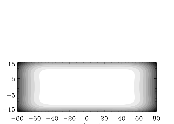
Figure 1: The potential energy experienced by an $\bar{\rm H}$ due to the spatially varying magnetic field. Every contour represents a change in energy of 10 mK $\times k_{B}$.

Figure 2: Evolution of the average energy of the $\bar{\rm H}$’s as a function of the detuning when the magnetic potential is that shown in Fig. 1. The linetypes are for when the laser is detuned $2\times$ the B-field free optimum value (solid line), $3\times$ detuned (dotted line), $4\times$ detuned (dashed line), and $5\times$ (dash-dot) line. The dash-dot-dot-dot line is for the optimum detuning when only the two end magnets are energized which leads to a trapping potential quadratic in $z-z_{mid}$.

Figure 3: Energy distribution of the $\bar{\rm H}$’s when the laser is detuned $4\times$ the B-field free optimum value and the trapping potential is that in Fig. 1. The different curves correspond to different time windows: 0-40 s is solid, 40-80 s is dotted, 80-120 s is dashed, 120-160 s is dash-dot, and 160-200 s is dash-dot-dot-dot.

Figure 4: Energy distribution of the $\bar{\rm H}$’s for the time window of 160-200 s when the laser is detuned $2\times$ the B-field free optimum value (solid line), $3\times$ detuned (dotted line), $4\times$ detuned (dashed line), and $5\times$ (dash-dot) line.

Figure 5: Same as Fig. 3 except that the initial energy distribution was a thermal distribution at 30 mK (current actual plots are for 50 mK until the data comes in). The inset shows the energy distribution in the final window (solid line) and a 20 mK thermal distribution (dotted line).

Figure 6: Same as Fig. 4 except that the initial energy distribution was a thermal distribution at 30 mK.

References

- (1) G. B. Andresen, et al (ALPHA Collaboration), Nature 468, 673 (2010).
- (2) G. B. Andresen, et al (ALPHA Collaboration), Nature Phys. 7, 558 (2011).
- (3) C. Amole, et al (ALPHA Collaboration), Nature 483, 439 (2012).
- (4) G. Gabrielse, et al (ATRAP Collaboration), Phys. Rev. Lett. 108, 113002 (2012).
- (5) M. E. Glinsky and T. M. O’Neil, Phys. Fluids B 3, 1279 (1991).
- (6) F. Robicheaux and J. D. Hanson, Phys. Rev. A69, 010701(R) (2004).
- (7) J.L. Hurt, P.T. Carpenter, C.L. Taylor, and F. Robicheaux, J. Phys. B 41, 165206 (2008).
- (8) F. Robicheaux, J. Phys. B 41, 192001 (2008).
- (9) T.W. Haensch and C. Zimmermann, Hyperfine Interact. 76, 47 (1993).
- (10) M.C. Fujiwara et al, AIP Conf. Proc. 1037, 208 (2008).
- (11) I. D. Setija, H. G. C. Werij, O. J. Luiten, M. W. Reynolds, T. W. Hijmans, and J. T. M. Walraven, Phys. Rev. Lett. 70, 2257 (1993).
- (12) V. Zehnle and J. C. Garreau, Phys. Rev. A63, 021403 (2001).
- (13) D. Kielpinski, Phys. Rev. A73, 063407 (2006).
- (14) S. Wu, R.C. Brown, W.D. Phillips, and J. V. Porto, Phys. Rev. Lett. 106, 213001 (2011).
- (15) K. Helmerson, A. Martin, and D.E. Prichard, J. Opt. Soc. Am. B 9, 1988 (1992).
- (16) H. J. Metcalf and P. van der Straten, ”Laser Cooling and Trapping”, Springer (1999).
- (17) K. S. E. Eikema, J. Walz, and T. W. Hansch, Phys. Rev. Lett. 83, 3828 (1999).
- (18) M. Scheid, D. Kolbe, F. Markert, T. W. Hansch, and J. Walz, Opt. Express 17, 11274 (2009).
- (19) T. Momose, private communication.
- (20) C. Amole, et al (ALPHA Collaboration), New J. Phys. 14, 015010 (2012).
- (21) E. Forest and R. D. Ruth, Physica D 43, 105 (1990).
- (22) H. Yoshida, Phys. Lett. A 150, 262 (1990).
- (23) J. Candy and W. Rozmus, J. Comput. Phys. 92, 230 (1991).