Real Second Order Freeness
and Haar Orthogonal Matrices
James A. Mingo(∗)Department of Mathematics and Statistics, Queen’s
University, Jeffery Hall, Kingston, Ontario, K7L 3N6,
Canada
mingo@mast.queensu.ca and Mihai Popa(∗)(‡)Department of Mathematics and Statistics, Queen’s
University, Jeffery Hall, Kingston, Ontario, K7L 3N6,
Canada, and
Institute of Mathematics “Simion Stoilow” of the Romanian Academy, P.O. Box 1-764, Bucharest, RO-70700, Romania
popa@mast.queensu.ca
Abstract.
We demonstrate the asymptotic real second order freeness of
Haar distributed orthogonal matrices and an independent
ensemble of random matrices. Our main result states that if
we have two independent ensembles of random matrices with a
real second order limit distribution and one of them is
invariant under conjugation by an orthogonal matrix, then
the two ensembles are asymptotically real second order
free. This captures the known examples of asymptotic real
second order freeness introduced by Redelmeier [r1, r2].
∗ Research supported by a Discovery Grant from
the Natural Sciences and Engineering Research Council of
Canada
Research supported by the Natural Science Foundation of China Grant No. 11150110456, and the Romanian National Authority for Scientific Research, CNCS UEFISCDI, Project Number PN-II-ID-PCE-2011-3-0119
1. Introduction
The large behaviour of random matrices has been actively
studied since Wigner’s celebrated semi-circle law was found
in 1955, [w]. Subsequently in 1967 Marchenko and Pastur
found the limit distribution for Wishart matrices
[mp1], now called the Marchenko-Pastur distribution.
The essential point of these discoveries is that for many
ensembles of random matrices the description of the
distribution of the eigenvalues gets much simpler in the
large limit. Much subsequent work has been devoted to
expanding and refining this work, see for example the recent
book of Anderson, Guionnet, and Zeitouni [agz].
Another direction of research in random matrices deals with
the interaction of independent ensembles of random
matrices. In this direction one studies the limit eigenvalue
distribution of sums and products of ensembles whose limit
distributions are already known. The direction was
discovered by Voiculescu in his work on free probability. In
[v1] and later in [v2], Voiculescu showed that
independent ensembles were asymptotically free if at least
one was unitarily invariant. Recall that if two random
variables are freely independent then there is a universal
rule for finding the mixed moments from the moments of the
individual random variables. One does this either
analytically by using the and transform, see
[vdn], or combinatorially using free cumulants, see
[ns].
In the last two decades the fluctuations of the eigenvalues
have been studied both in the physics and the mathematics
literate, see e.g. [az, bs, fmp, j, k, kkp]. In
[mn] it was shown that the fluctuations of Wishart
matrices could be analyzed using the non-crossing diagrams
introduced in [s], but by using an annulus instead of a
disc or line, see Figure
1, hence all the
combinatorial techniques developed by Nica and Speicher
[ns] could be brought to bear on the study of
fluctuations. Thus motivated, second order freeness was
introduced in [ms, mśs] and later higher order freeness
in [cmśs].
The point of second and higher order freeness is that it
enables one to do for fluctuation moment and higher order
trace-moments what Voiculesu’s first order freeness did for
moments. In particular if two random variables are second
order free and one knows the moments and the fluctuation
moments of each variable then there is a universal rule for
finding fluctuation moments of sums and products, see
[mst].
In [cmśs, mn, ms, mśs] the random matrices considered
were either Hermitian or unitary. This left the question of
how to deal with real symmetric and orthogonal matrices. On
the first order level the techniques of Voiculescu were
equally applicable to real and complex ensembles. However it
was shown in [r1, r2] that the universal rule found in
[ms] needed to be modified for the real case; in
particular the transpose of the various operators made an
appearance. This led to a new kind of second order freeness,
called real second order freeness in [r1, r2].
The non-crossing diagrams introduced in [mn] had to
augmented by diagrams in which the orientation of one of the
circles was reversed. The operators on the reversed side get
transposed. One can give a heuristic interpretation of this
using maps on surfaces, see [lz]. In the complex case
we only work with orientable surfaces and in the real case
we also have to also deal with non-orientable surfaces. So
we imagine that our surfaces are marked our operators and
the graphs tell us how they get multiplied, see Figure
5. Wherever we put an operator on
the front side of the surface, we put its transpose on the
back. The non-orientability of the surface means that we can
cross from font to back and see the transposed operators,
something that we cannot do in the complex case.
The main result of this paper, Theorem
54, asserts that if and
are independent ensembles of random matrices and
if at least one of them is invariant under conjugation by an
orthogonal matrix then the ensembles are asymptotically real
second order free. The proof of this theorem occupies nearly
the whole paper. This theorem is the orthogonal version of a
theorem in [mśs], where we assumed that one of the
ensembles is invariant under conjugation by an unitary
matrix. While the statements of the two theorems are similar
the proofs follow quite different paths. In [mśs] the
asymptotics of the cumulants of the unitary Weingarten
function, from [c], were heavily used. In this paper we
only need the multiplicitivity of the leading order of the
orthogonal Weingarten function, see [cs]. We work with
centred elements and this obviates the need to work with the
cumulants of the Weingarten function.
Illustrative examples
Let us conclude this introduction with some
examples. Suppose that are
deterministic matrices and is a Haar
distributed random orthogonal matrix and be a Haar distributed random unitary matrix. From
[mśs, Prop. 3.4] we have
So we already see a bit a difference between the orthogonal
and unitary cases; namely the appearance of transposes in
lower order terms. When we consider covariances we see more
differences. First in the unitary case we have
Now in the orthogonal case we have
Note the similarity to the unitary case except that each
term of leading order appears twice–once with no transposes
and once with transposes on and . Moreover when
the ’s are centred, i.e. , the only
remaining terms are and
. These terms correspond to
spoke diagrams which are discussed in the next section, see
Figure 2. By working with
centred elements the number of terms is significantly
reduced, it is in this way that we can skip the calculations
requiring the cumulants of the Weingarten function.
The Organization of the Paper
In section 2 we review the
definitions of non-crossing partitions. In section
3 we use the Weingarten function
of [cs] to compute the trace of a product of orthogonal
matrices and independent random matrices. This is how the
calculations in the examples above were done. In section
4 we prove two important lemmas on
a special kind of non-crossing partition called a spoke
diagram. These are the only diagrams that survive in the
large limit. In section
5 we recall the notions
of second order freeness from [r1, r2] and prove that
real second order freeness satisfies an associative law. In
section 6 we prove that Haar
distributed orthogonal matrices and an independent ensemble
are first order free. That this could be done was already
suggested by Voiculescu in [v1] some twenty years ago
and was later proved in [cs, Thm. 5.2]. In section
7 we show that the
fluctuation moments of Haar distributed orthogonal matrices
and an independent ensemble of random matrices satisfy the
universal rule required for second order freeness. In
section 8 we show that the third and
higher cumulants of traces of products of Haar distributed
orthogonal matrices and an independent ensemble of random
matrices satisfy the final condition for asymptotic real
second order freeness. This completes the proof of their
asymptotic real second order freeness. In section
9 we use this result to obtain all
our other results on asymptotic real second order freeness.
In section 10 we present some
concluding remarks and indications of future work.
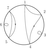
2. Non-crossing diagrams and pairings
Central to the combinatorial approach to freeness is the
idea of a non-crossing partition. A partition of is
non-crossing is one in which the blocks can be drawn in a
non-crossing way; see the left half of Figure
1. For second order
freeness we need non-crossing annular partitions. This means
we can draw the blocks on an annulus in a non-crossing way;
see the right half of Figure
1. In the case of second
order freeness additional information about the partitions
is needed, namely the order in which they visit the
points. For this reason we regard our partitions as
permutations by interpreting the blocks of the partition as
cycles in the cycle decomposition of the corresponding
permutation.
Notation 1.
For any integer , let . Let be the set of all partitions of
. For any partition of let denote
the number of blocks of , and . The set is a partially ordered set in
which means every block of is
contained in some block of . With this order
is partially ordered set and is in fact a
lattice. We denoted the join of two partitions and
by .
Given a permutation it can be difficult to decide if there
is a non-crossing way of drawing its cycles, however there
is an algebraic way to see if such a diagram exists. Let
and let be a
permutation of and denote by the subgroup of generated by and
. If the subgroup acts
transitively on then we have that is
non-crossing if and only if
(1)
Note that the condition that
act transitively is the same as requiring that there is at
least one cycle of that contains points in both cycles
of . When this happen we shall say that
connects the cycles of
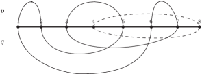
Figure 1. On the left
we have the non-crossing disc permutation . On the right we have the non-crossing annular
permutation .
We can extend this to the case of having any number
of cycles. Let and be permutations of
. Let be the number of orbits of . Then
(2)
with equality only if is non-crossing with respect to
, see e.g. [mn, Remark 2.11].
In the case of real second order freeness we require an
additional set of non-crossing diagrams, we call these
reversed non-crossing annular permutations. If we
let
then we say that a permutation is a
reversed non-crossing permutation of a -annulus if
Notice that this is the same condition as in Equation
(1) but is replaced with
. Graphically, this corresponds to using the same
orientation for labelling the points on each circle; see the
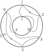
right hand side of Figure 2.
A special kind of a non-crossing annular permutation that we
shall make use of is that of a spoke diagram, see
Figure 2. Recall that a
pairing of is a partition in which each block
has two elements. We usually regard a pairing as a
permutation, by considering each block to be a cycle with
two elements. By a standard spoke diagram we mean
a non-crossing pairing of an -annulus in which all
pairs connect the two circles. Note that means that
and there is such that such that
every cycle of is of the form for
.
By a reversed spoke diagram we mean a reversed
non-crossing annular pairing in which all blocks connect the
two circles; see Figure 2. By a
spoke diagram we mean either a standard or reversed
spoke diagram. See Figure
2. Note that means that
and there is such that such that
every cycle of is of the form for
.
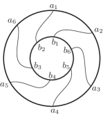
Figure 2. On the left we
have a non-crossing pairing of a -annulus in which
all blocks connect the two circles, i.e. a standard spoke
diagram. Note that the two circles have opposite
orientations. In the figure on the right we have a
reversed non-crossing pairing of a -annulus. i.e. a
reversed spoke diagram. Note that the two circles having
the same orientation.
We denote by the pairings of . If is a
pairing of and is a cycle of we shall
denote this by . We denote by
the set of all standard spoke
diagrams and by the set of all
reversed spoke diagrams.
Given a permutation , we shall frequently
consider the cycles of as a partition of . This
map forgets the order of
elements in a cycle and so is not a bijection. Conversely
given a partition we put the elements of
each block into increasing order and consider this a
permutation. Restricted to pairings this is a bijection.
3. The Trace of a Product
Given a permutation and
matrices we let be the
-entry of and
(3)
This expression can also be written as a product of traces
as follows. Write in cycle
form. If is a cycle of we
let . Then
Let be a Haar distributed random
orthogonal matrix and be
random matrices whose entries have moments of all
orders. Let be a permutation, and let
. In this section we wish to find a simple expression
for
We shall use the Weingarten function introduced by Collins
and Śniady [cs]. The Weingarten expresses the
expectation as a
sum over pairings of . The first question we need to
address is, for two pairings and , the relationship
between the cycles of and the blocks of . See
Figure 3. This is a standard fact;
for the reader’s convenience and to establish our notation
we give a proof.
Lemma 2.
Let be pairings and a cycle of . Let . Then is also a cycle of , and these
two cycles are distinct; is a block of and all are of this form;
.
Proof.
We have , thus . Hence . If and were to have a non-empty intersection then,
for some , would have a fixed point, but this
would in turn imply that either or had a fixed
point, which is impossible. Since and , must be a block of . Since
every point of is in some cycle of , all blocks
must be of this form. Since every block of is the
union of two cycles of , we have .
∎
Notation 3.
Let and . Let be the permutation of
which sends to for . Since each
cycle of is of the form , we shall also
regard as a pairing of . If , let denote the
permutation of given by .
Given a permutation on we shall regard
also a permutation of where for ,
we let . Let be the permutation
of with the one cycle , but
following the convention mentioned above we also have
for .
Figure 3. In this example , , and . Then
and .
Lemma 4.
Let be pairings then .
Proof.
Note that for we have
and . Thus the elements in an orbit of
always alternate in sign. Moreover . Hence the positive elements of a cycle of form a cycle of . Conversely let be a cycle of . Then is a cycle of . This establishes a bijection between the cycles of and the cycles of .
∎
The pairings of shall be denoted . For a pairing , and a -tuple
we write to mean that whenever we have . For
a matrix let , the
transpose of , and . For and , let
Lemma 5.
Let . The there is and
such that
Proof.
We saw that the cycle decomposition of may be
written where . It is arbitrary which of the pair
is called and which .
For each , choose a representative of each pair , say . For each we
construct a cycle as follows. Suppose . Let where
Note that . Then we let and .
We denote the entry of by
. Let be a cycle
of . Let and be as above i.e. and . Then
Thus
Note that , as . Thus
∎
Remark 6.
The pair constructed in Lemma
5 is not unique; however
since
the value of is independent of the choices made.
Notation 7.
Let be the inner product vector space with
orthonormal basis . For an integer ,
define
by
In [cs, §3], Collins and Śniady showed that
is an invertible linear transformation and denoted its
inverse , the orthogonal Weingarten
function. From the construction, is always a rational function of . Collins and
Śniady showed [cs, Thm. 3.13] that given if we expand in power series in then we
have
(4)
Remark 8.
It was shown in [cs] that the coefficient of can be written as a product of signed
Catalan numbers. Indeed, write and
factor into a product of cycles . Let
be the Catalan number
. Then the coefficient of is
where the cycle has elements.
The reason for introducing is its use in computing
matrix expectations. For pairings , is a pairing of . For a pairing
of and we let if whenever
is a pair of and 0 otherwise.
Let be a Haar distributed orthogonal matrix
and a non-zero integer. Then
Proof.
Let be the permutation with the one cycle
. If is odd then . So suppose that is even. First let us consider
where is the -tuple . Now . Thus
only when is constant on the blocks of . Hence
Thus . But . Hence .
∎
Notation 11.
Let be a permutation of but, as in
Notation 3, considered as
a permutation of by setting for
. Given and we consider the pairing of given by
of . By Lemma
5 there is a permutation
and
such that
Note that is a pairing of , is a
pairing of and so is a pairing of
. If we adopt the notation then . Recall from the proof of Lemma
5 that was obtained by writing as a product of cycles and
taking one cycle of each pair . After this
choice has been made
records the position of the minus signs.
Proposition 12.
Let be a Haar distributed random orthogonal
matrix and random
matrices which are independent from and whose entries
have moments of all orders. Let , and suppose .
Proof.
Now for notational convenience let and let , then
. Thus
(5)
where if . Also . Hence we
have
Let . Then . Thus as we have
So
∎
We shall need a special case of this result in section
9. Let us say that a permutation
is parity preserving if for all ,
and have the same parity.
Lemma 13.
Let be even positive integers and . Let . Suppose that
is such that . Then for all , is
parity preserving.
Proof.
We first show that is parity preserving. By direct computation we have
the following.
Note that since always reverses the parity of its
argument, all four possible outcomes are odd. Thus
takes odd numbers to odd numbers. Since is a
permutation it must then take even numbers to even
numbers. Indeed
Now is parity preserving, thus so is
. Finally is obtained by choosing
one representative of each pair of , and taking the absolute value
of each entry. This means that each cycle will consist of
integers of the same parity. Hence is parity
preserving.
∎
We wish to extend the conclusion of Proposition
12 to case where some of the
’s are not interleaved by orthogonal matrices.
Proposition 14.
Let be a Haar distributed random orthogonal
matrix and random
matrices which are independent from and whose entries
have moments of all orders. Let , , and suppose .
Proof.
The proof is the same as for Proposition
12 except that we append the
random variable to the right
hand side of each expression.
∎
We now wish to extend the conclusion of Proposition
12 in another way, namely to
the case of independent Haar distributed orthogonal
matrices. Suppose are independent Haar
distributed orthogonal matrices, with the
entry of denoted . We shall need
a expression for extending that given in Theorem
9.
Notation 15.
Given an -tuple of integers in
we let be the partition of such that
where and are in the same block of
and when and are in
different blocks of .
Let be a partition of and be a pairing such that each pair of lies in
some block of . We shall denote this by . If we write the blocks of as , then the pairs of that lie in form a
pairing of which we shall denote by or just
when convenient.
If we have a partition and pairings with then we let
Remark 16.
Note that since is not multiplicative,
and are different. However by
Remark 8 we see that when then as the leading terms in both
expressions are the same.
Lemma 17.
Suppose are independent Haar
distributed orthogonal matrices. Let the
entry of be denoted . Given an
-tuple in then
Proof.
We can write as a product of expectations,
one for each block of . For each block of
we get a factor where is the restriction of to
the block . Taking the product of these terms we get
.
∎
Proposition 18.
Let be independent Haar distributed orthogonal matrices and
random matrices which are independent from and whose entries have moments of all orders. Let
, and suppose . For each -tuple in we have
Proof.
The only point where the proof differs from the proof of
Proposition 12 is in Equation
5, which we replace
by
The remainder of the proof is unchanged.
∎
4. A Lemma on Spoke Diagrams
At several points later on we shall wish to know that a
given permutation represents a spoke diagram (see Figure
2). Lemma
20 identifies standard spoke
diagrams and Lemma 21
identifies reversed spoke diagrams.
Lemma 19.
Suppose is a permutation,
a pairing, and an assignment of
signs, are such that is a pairing. Let be a pair of .
i)
If then , , and
.
ii)
If then , , and .
Proof.
(i)
Let us suppose that . Since and we have
Since is a pairing, is also a
pairing — recall that . Also
Thus , because is a pairing. Since both
we have that . Moreover and so . Unwinding this equation we have
Since , as a permutation, doesn’t change
the sign of its argument, we have . Thus , and we are left with
is a cycle of ,
, and
as
required.
(ii) Let us suppose that . Since and we have
Since is also a pairing, is a
pairing. Also
Thus is a pair of
. Thus
. Moreover
. Unwinding the equation we have
Since , as a permutation, doesn’t change
the sign of its argument, we have . Thus , and we are left with
is a cycle of ,
, and
as claimed.
∎
Lemma 20.
Let be the permutation with the two cycles , let , and let be a pairing such
that
i)
, i.e. at least one of cycle of
connects the two cycles of ;
ii)
for some we have ; and
iii)
is a pairing.
Then , and are standard spoke
diagrams, and there is , which we make take to be
if we assume that , such
that
a)
every cycle of is of the form for , and
b)
every cycle of is of the form
for ,
c)
and for all
,
d)
for all .
Proof.
Let , i.e. is a cycle of , and
suppose . By using induction on
Lemma 19 we know that for
all , ,
, and
. Recall
that in the proof of Lemma
19 (i) we showed
that . This implied
that and that
. By our induction
argument we have that for all .
By assumption, has at least one pair that
connects the cycles of ; and so by what we have just
observed, all cycles of connect the two cycles of
. This implies , and all cycles of are of
the form , where ,
assuming . Moreover, both and
are spoke diagrams, i.e. non-crossing annular
pairings of an -annulus with all pairs connecting the
two circles; see Figure 2.
∎
Lemma 21.
Let be the permutation with the two cycles , let , and let be a pairing such
that
i)
, i.e. at least one of cycle of
connects the two cycles of ;
ii)
for some we have ; and
iii)
is a pairing.
Then , and are reversed spoke
diagrams, and there is , which we make take to be
if we assume that , such
that
a)
every cycle of is of the form for , and
b)
every cycle of is of the form
for ,
c)
and for all
,
d)
for all .
Proof.
Let , i.e. is a cycle of , and
suppose . By using induction on
Lemma 19 we know that for
all , ,
, and
. Recall that
in the proof of Lemma 19
(ii) we showed that . This implied that
and that
. By our induction argument we
have that for all .
By assumption, has at least one pair that
connects the cycles of ; and so by what we have just
observed, all cycles of connect the two cycles of
. This implies , and all cycles of are of
the form , where ,
assuming . Moreover, both and
are spoke diagrams, i.e. non-crossing annular
pairings of an -annulus with all pairs connecting the
two circles; see Figure 2.
∎
Corollary 22.
Let be a permutation, a
pairing, and an assignment of
signs. Suppose that is a pairing then each block
of contains at most two cycles of .
Proof.
We saw in Lemma 19 that
when connects a pair of cycles of these two
cycles form a spoke diagram. So a block of
can contain at most two cycles of .
∎
5. Real Second Order Freeness
Let us recall the definition of real second order freeness
from Redelmeier [r2, §1]. We begin with the concept of a
real second order non-commutative probability space.
Definition 23.
Let be an algebra over and with an
anti-automorphism of order 2 denoted by . Suppose that is a tracial
state and is a
bi-trace, i.e. is bilinear and tracial in each
entry. Moreover we assume that , and for all . Then is a real second order
non-commutative probability space.
Notation 24.
Let unital subalgebras be given.
i)
We say that a tuple of elements from
is cyclically alternating if, for each , there is
such that and,
if , we have for all . We count indices in a cyclic way modulo ,
i.e., for the equation above means .
ii)
We say that a tuple of elements from
is centred if we have
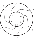
Definition 25.
Let be a real second order
non-commutative probability space and suppose that we have
unital subalgebras that are
invariant under . We say that are real free of second order if (see figure 4)
i)
the subalgebras are free with respect
to ;
ii)
for every and such that and are centred and cyclically alternating, we
have
a)
, if or if and and are from different subalgebras;
b)
for we have, taking all indices
modulo
(6)
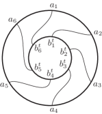
Figure 4. The terms on the right
hand side of equation
(6) are sums over all
spoke diagrams. In the diagram on the left the circles
have the opposite orientation; we put the ’s on on
circle and the ’s on the other. This gives the first
term on the right hand side of
(6). In the circle on
the right the two circles have the same orientation and we
put ‘’s on the inside circle. This gives the second
term on the right hand side of
(6).
Notation 26.
Let be a
polynomial in the non-commuting variables and be matrices. By we mean the
matrix obtained by replacing by and by
in . Similarly if is a
real second order non-commutative probability space then by
we mean the random variable in
obtained by replacing by and by .
Remark 27.
Expanding on the notation in equation
(3) we define, for a permutation
and , as below.
where
the product is over all cycles of and for each
cycle we get the factor
. This makes a
-linear functional.
With this notation we can write equation
(6) in a simpler way:
where, recall, denotes the set of standard spoke
diagrams and denotes the set of standard spoke
diagrams.
We shall need to use the associativity of real second order
freeness. Let us recall how this works in the first order
case [vdn]. Suppose that we have unital subalgebras
which are free with
respect to . Moreover that for each
we have unital subalgebras which are free with respect to . Then
by [vdn, Prop. 2.5.5 (iii)] the subalgebras
are free with
respect to . We shall prove the real second order
version of this. In [mśs, Remark 2.7] the second order
version of [vdn] was left as an exercise for the
reader, now we shall provide a solution. We begin with a
lemma.
Lemma 28.
Let be unital subalgebras
which are free with respect to . Suppose that are such that
for all and ;
and ;
and .
Then for , and for
Proof.
Let us begin by showing that
First suppose that . Then both and are 0 by
freeness. Thus both sides of the equation above are 0. Next
suppose that and write . Then because . Thus
Now we conclude by induction. If we get the formula we
claimed. If then
by the freeness of the ’s. The case when is
exactly the same.
∎
Proposition 29.
Let be -invariant
unital subalgebras of which are real second order free
with respect to . For each
suppose we have -invariant unital subalgebras which are real free of
second order with respect to . Then the
subalgebras are
real free of second order with respect to .
Proof.
The proof of first order freeness is as in [vdn, Prop. 2.5.5
(iii)]. So let us prove part (ii)
of Definition 25. Let
be such that
for all and ; and
and ; and
and .
We must show that for
(7)
and is 0 for ; the case is immediate.
Note that adjacent ’s are, by assumption, from
different ’s but might be from the same
. So we group the ’s according to which
contains them. Let be positive integers
such that and ,
for and . Then we let . Then .
We do exactly the same for the ’s. Namely we let be positive integers such that and for and
. We let
. Then .
Note that by first order freeness
since the ’s are first order free by
[vdn, Prop. 2.5.5 (iii)]. Likewise .
If then we have
(7) by the assumed second
order freeness of . If , then by the assumed second order freeness of
we have , thus the left hand side of
(7) is 0.
Let us consider the right hand side of
(7). If then the
right hand side is 0. So let us suppose that . Let us
first consider the term involving . For and we must have for all
. This means gives a bijection between
the ’s which contain the ’s and the ’s
which contain the ’s. So in particular , which
is impossible. Likewise if then we have
a bijection between the ’s containing the ’s and
the ’s containing the ’s. So again we would
have .
Now let us suppose that . By the assumed real
second order freeness of we have
and 0 when . Thus for this , assuming
for all , we have
where is the spoke diagram
obtained by matching up with
.
If we let run over on the right hand side
of (8), the corresponding
’s will not exhaust all ’s on the right hand
side of (7), but the ones that
are missed are such that , by the first order freeness of the
’s. Similarly for the ’s in on the
right hand side of (8). We thus
have
Suppose for each we have random matrices . We say that the ensemble has a
real second order limit distribution if there is a
real second order non-commutative probability space and such that
for all polynomials in the
non-commuting variables we have
i)
;
ii)
iii)
for all
Remark 31.
The third condition is only needed to ensure the convergence
of fluctuations of mixed moments. In fact boundedness would
be enough. For many ensembles of matrices the
cumulant vanishes on the order of , for example the
ensembles discussed in [r1, r2]. For deterministic
matrices the higher cumulants of traces are 0. Moreover a
close reading of our proof shows that if one starts with an
ensemble with between and
for , the mixed cumulants of ’s and
’s for would have the same order as
.
Remark 32.
Suppose we have for each , random matrices , a non-commutative probability space
, and such that for
every polynomial in the non-commuting variables we have
then we say that the matrices
have the limit joint -distribution given by
.
Definition 33.
Let and be two ensembles of random matrices such that
has
a real second order limit distribution given by in the real second order
non-commutative probability space . If the two unital subalgebras and are real free of second
order then we say that the two ensembles and are
asymptotically real free of second order.
6. First Order Freeness of Haar Orthogonal
and Independent Matrices
To show that a family of random matrices and an independent family of
orthogonal matrices are asymptotically real free
of second order, we must first demonstrate that they are
asymptotically free of first order, or asymptotically free
in the sense of Voiculescu [vdn, §2.5].
For this we must show that given polynomials in and such that
and random matrices
with , then
provided that the entries of the ’s are independent
from those of the ’s and the have a real second order limit distribution. For
this it suffices to prove that
for any sequence of non-zero integers and
as above.
Notation 34.
Let be a permutation and be a
partition such that each cycle of lies in some block
of . We denote this relation by . Let
be random matrices and write,
as in equation (3),
Let the blocks of be and let
be the product of cycles of that lie in
. If is a cycle of , let
. If
, as a product of cycles, let
. Next let
(9)
Finally for and , let
To make this clear let us give an example. Let , and . Then
We shall also need to work with the normalized trace . We let .
If and , in the sense above,
then we let
(10)
Then by Möbius inversion we have
(11)
Remark 35.
In what follows, for an ensemble of matrices , will suppress the dependency of
on and just denote it by . Moreover the
-entry of will be denoted . This
should not cause any confusion as at each stage of the
discussion we shall only be multiplying matrices of the same
size. Likewise for an ensemble of random orthogonal
orthogonal matrices , we shall drop the
dependence on from the notation.
Theorem 36.
Let for each , be a
ensemble of centred random matrices that have a
real second order limit distribution, a Haar distributed
random orthogonal matrix, and
be non-zero integers. Then
Proof.
In order to be able to use the result of Proposition
12, with , we have to reduce it to the case of each
being either or . We can achieve this by
inserting an identity matrix, , between any two adjacent
’s or adjacent ’s. For example
would become . So with this change we
must show that, whenever we have and random matrices with a limit joint -distribution such that for
each , either is centred, i.e. ,
or and , then
Let us recall the construction of . We write the permutation , which is the product of two
pairings, as a product of cycles. We showed that the cycles
always occur in pairs of the form , where . From each pair we choose one, and
then from this we obtained a cycle of by deleting any minus signs. The
minus signs that are deleted are recorded in . So
let us consider the singletons of . If is a singleton of
, then will have the two singletons
and thus will be a cycle of and hence will be a cycle of . The cycles of are either cycles
of , consisting of pairs of positive numbers, or cycles
of , consisting of pairs of negative
numbers. Thus if is a singleton of
then we must have
, and hence is a
centred matrix.
Now consider the expansion
We have
We must next find a upper bound for the order of
Since has a real second order limit
distribution we have that
where is the number of blocks of that contain a
single cycle of . If has a singleton then
, too, will have a singleton and then will
be centred so will have a factor , hence
.
Thus and so , thus
Thus
and hence
∎
Corollary 37.
Let be random
matrices whose entries have moments of all orders, a
Haar distributed random orthogonal matrix,
independent from , and
. Suppose that for
each we have that either or and
(using ), and . Then
in fact
(12)
where the sum is over all ’s such that is a
pairing and
Proof.
The first claim is just the second last equation of the
proof of Theorem 36. Recall
that when we expand into cumulants
and let be the number of blocks of that contain a
single cycle of we have with equality only when and ,
i.e. and is a pairing. This
establishes the second claim.
For the moment let us fix and let
be the permutation which fixes
and whose restriction to is . Likewise let
and . Then Then we expand as above
Suppose is such that
and . Then
where is the number of blocks of that contain only
one cycle of . Since, by assumption,
, the last cycle of cannot
be in a block of on its own (otherwise );
thus . As in the proof of Theorem
36,
and as the cycle cannot be on its own we have
. So . Thus and so
Since this holds for every we have
Since this in turn holds for every and we have
∎
7. Fluctuation Moments of Haar Orthogonal
and Independent Random Matrices
Our next step is to show that the limit distribution of Haar
distributed orthogonal matrices and an independent ensemble of random
matrices with a real second order limit distribution
satisfies part (ii) (b) of Definition
25. Fix positive integers
and and let be the permutation with the two
cycles .
Theorem 38.
Let and be a ensemble of centred matrices
that have a real second order limit distributions given by
and , respectively,
in a real second order non-commutative probability space
, and a Haar distributed
random orthogonal matrix, and non-zero integers. Suppose that the
entries of are independent from those of . Then
exists and equals 0 when , and when ,
equals
(13)
where the indices of the ’s and ’s are taken modulo
.
Proof.
We begin
by noting that by Theorem 9,
must be even, otherwise the limit of the covariances
is 0. In order to apply Proposition
12 to the expression
we have to reduce it to the case where all ’s and ’s
are either 1 or . So let us consider the term
of expression
(13). In order for this to be
non-zero we must have . So when we
perform the reduction used in the proof of Theorem
36 we replace ,
supposing , with and
with the factor
gets replaced by . Likewise
with the factor . Thus without loss of
generality we can assume that . In this case we must show that
exists and equals 0 when and when
equals
(14)
where the in the index of the second in
is the
permutation with cycle decomposition .
We shall show that the first term
(17) converges to
and the second (17) and third term
(17) converge to 0.
We first consider expression (17),
and show that this has the limit we have claimed. Let us
find the order of ; to do this we have to rewrite this
expectation in terms of cumulants so that we can use our
assumptions about the ’s and ’s having a real second
order limit distribution. If we consider a
partition of then by equation
(11) we have
(18)
Suppose and . If
has a singleton , then is also a singleton of
. As in the proof of Theorem
36, this implies that
(or if ) is centred, and thus,
. Thus we only have to consider ’s with no
singletons. Hence . Suppose is a
block of which contains two or more cycles of
; the corresponding factor in Equation
(18) is a second or higher
cumulant of traces, which converge by our assumption that
the ’s and ’s have a real second order limit
distribution. Hence these factors will be of order
. Each block of which contains only one
cycle of will be of order . Hence
where is the number of blocks of which
contain only one cycle of . As
we have and the order can only be
achieved when , which implies that , as partitions, and no cycle of is a
singleton, because no block of is a singleton. If
and has no
singletons; must be a pairing. Combining these
conclusions we have
unless and is a pairing, in which case
(19)
Using our usual bound on the order of , namely
we thus have
unless and is a pairing, in which case
Thus
(20)
where the second sum runs over all such that and is a pairing. To find the
limit as we use Lemmas
20 and
21.
First suppose that there is such that
. Then by Lemma
20 we have , every
cycle of connects the two cycles of , and
for all . Then for
some we have . Again by Lemma
20 we have for all
,
,
.
Thus and
(21)
which converges to
as .
Next suppose that there is such that
. Then by Lemma
21 we have , every
cycle of connects the two cycles of , and
for all . Then for
some we have . As in Lemma
21, let . Then , for . Hence by Lemma
21 we have for all
To show that (17) and
(17) vanish as we have to consider the order of
with
. As before we write this as a sum of
cumulants
Let be the number of blocks of that contain only
one cycle of . If has a singleton then the
corresponding cumulant will be 0 because the ’s and ’s
are centred; so we only consider ’s which have no
singletons and thus . If we let be
the number of blocks of that contain exactly one cycle
of , then
and . Recall that
where . Now let
us use Notation 34 to write this
as
If has a singleton then will have a
singleton . As in the proof of Theorem
36 this singleton must be a
centred (or if ). So if has a
singleton we must have
. Thus we may assume that has no singletons, so in
particular . . As before let be
the number of blocks of that contain exactly one cycle
of . Then
Now and, as usual,
Thus
Since and we must have , as equality would force as
partitions. Thus . Hence
Summing over all ’s we have
∎
Remark 39.
The proof of Theorem 38 actually
proves a stronger statement than was claimed. Let is an ensemble of centred random
matrices where for we let for we let for . Suppose that for any monomials , we have
where the indices of the ’s and ’s are interpreted modulo .
Corollary 40.
Let be a Haar distributed random orthogonal
matrix. Then for integers and
Proof.
Let and
. Let
be the permutation with the two cycles . Then by Proposition
12
and if let be the partition with blocks the cycles of
By the multiplicativity of the coefficient of the term of
leading order of we thus have
As in the proof of Theorem 36,
if has a singleton then , which is impossible given our
construction of . Thus has no
singletons. Hence . Thus
, with equality
only if and is a pairing.
Let . Either or
. As in the proof of Theorem
38 all cycles of connect the
two cycles of and hence . Also in the
case in which , we have
. There are exactly
such ’s. In the case , we have
. There are exactly
such ’s. All together there are such
’s. By Remark 8 the coefficient
of in is 1. This gives
the claimed result.
∎
8. Vanishing of Higher Cumulants of Traces
Let be a family of random
matrices, containing the identity matrix, with a real second
order limit distribution. By this we mean that as
(23)
Let be a Haar distributed random orthogonal
matrix whose entries are independent from those of . In this section we shall show that whenever be random variables where each is one
of the following types:
(24)
The the third and higher cumulants of the ’s will
converge to 0 as . This, combined with
Theorems 36 and
38 will show that we have
asymptotic real second order freeness of the and
.
For the rest of this section we shall assume that the satisfy condition (23) and our
goal is to prove the theorem below.
Proof of Theorem
41 using Theorem
42: We begin by
recalling that the cumulant will be
0 whenever an is constant and . Recall also
that by our assumption of a second order limit distribution
is a convergent function of and thus
bounded. Thus if then
so does .
Suppose for some . Let . Let . Then
and .
Then and so
So we may suppose that any ’s of the form are centred.
Next suppose that , with each and whenever
we have . For each ,
we shall write as a linear combination of a constant
random variable and terms of the form , or
where for
each either or and
; where . We then
replace in by this linear
combination and get a sum of cumulants in which all the
’s are of the form (26).
To show that each can be written as such a linear
combination we replace for each , with
. We then expand this
sum. If we have a factor , we will get
cancellation of cyclically adjacent ’s wherever . This might bring two centred ’s next to
each other. As the product will not necessarily be such the
expectation of the trace is 0, we repeat the centring
process and continue. Since the number of factors decreases
whenever there is a cancellation, the process terminates
with either: an of the form
(26,i); an as in
(26.ii); or a constant
(if all the ’s get cancelled). ∎
Remark 43.
To illustrate the previous theorem let us consider the
example
There are six ’s and we let
with . This produces terms, some
of which are 0 because some of the entries of the cumulant
are constant. For example we shall get terms such as
If we started with the example
then we would also get terms like
where there no ’s.
Our task now is to prove Theorem
42. We shall recall the
moment cumulant relation
(27)
So to prove something about the cumulants we shall prove something first about and use this to prove
Theorem 42. We let
be the partitions of with blocks of
size either 1 or 2.
By Corollary
37 we have that is is of type
(26.ii) and
if is of type
(26.i). If and
are both of type
(26.ii) then by Theorem
38, . If they are both of type
(26.i), then by assumption
(23) we have . If is of type
(26.i) and is of
type (26.ii), then
, as
. Then by Corollary
37, . So in all cases and
are of order at most .
Where is all the partitions in
except those in and , the
partition with only one block. If then has blocks of size 1 or
2 and at least one block of size between 3 and . Since
the cumulants from the blocks of order and, by our
induction hypothesis, all others are of order ,
the product is of order
. Hence
forces us to conclude that . ∎
Notation 45.
From now on we shall assume that we have positive integers
. We let . There is
such that for we
have . We let be the permutation
with cycles
If then is the identity
permutation. We shall assume the random variables are
such that for
where for each either
or and ;
and for
and .
Let . If is odd and
positive then . So we shall assume
that is even, and possibly 0. Let be
the set of partitions of whose restriction to is
a pairing and all of whose other blocks are singletons. In
the case we have and the only partition in
is the one with blocks of size 1. We
assume that with for
.
Now let and be in . Then is a permutation of whose restriction to
is a pairing and all of whose other cycles are
singletons. Now consider . Its restriction to
consists of singletons. Its
restriction to is as in Notation
11, i.e. the cycles occur in
pairs . We obtained a permutation, , of
as follows. For each pair we choose one
representative, replacing any negative entries by their
absolute values. Now we wish to extend this construction to
the case where . The cycles in
also occur in pairs
(with ) and so we just choose for each of these
cycles. Also for let .
Let follow the notation used in Equation
(9). If is a partition
on and any permutation of we write
to be the product
, where the
blocks of are and . We likewise let be the product of cumulants along the blocks of
, see equation
(10). Recall that we then have
the moment-cumulant relation
(29)
By our assumption (23) on the
existence of a real second order limit distribution of the
’s we have
where is the number of blocks of that contain only
one cycle of . Suppose . Then any block of
that contains a single cycle of must
contain a cycle of , as
for . Thus . Also
recall, from the fourth paragraph of the proof of Theorem
36, that if is a
singleton of then , and
hence . So for any block of that contains
only one cycle of , must contain at least two
elements. Thus . We can only have when
every block of contains one cycle of
and that cycle has two elements,
i.e. is a pairing. This proves the first
claim.
If is a pairing then we have just seen
that to have we must have . Thus if we only consider ’s for which
we have
Finally we add back the remaining terms to obtain that
∎
Notation 47.
Suppose we have and and
as in Notation 45. Let
be the set of partitions such that is a pairing,
the condition being vacuously satisfied when . For let
Also if (i.e. ) we get the
same conclusion. When and is a
pairing, then and
because .
∎
Proof of Theorem
44:
To prove the theorem we show that
(30)
and then apply Corollary 48. We saw in
the proof of Theorem 42
that if is of type
(26.i) and is of
type (26.ii) then
, so on the left hand
side of (30) we only have to consider
’s for which each block is either contained in or
in . Thus
because cumulants corresponding to blocks of size three or
larger are and cumulants corresponding to blocks of
size two are and cumulants corresponding to blocks
of size one are 0.
Let us next show that
(31)
If we multiply these last two equations we get equation
(30) as
To prove (31) we use
(12) and
(18). They say that a first
and second cumulant of ’s if type
(26.ii) can be written, up
to terms of order , as sums over pairings
in unions of intervals of for which is a
pairing. Moreover by Corollary
22 if is a
pairing and is also a pairing then at most two
cycles of can be contained in any block of .
Let be a pairing such that is a
pairing. The partition determines a
partition of the cycles of .
By Corollary 22, . Thus we can write
Now is a product of first and
second cumulants. For each first cumulant, , we
apply equation (12) to write
with running over pairings of the corresponding cycle
of such that is a
pairing.
For each second cumulant we apply equation
(18) to write
with running over pairings that connect the corresponding union
of two cycles of such that
is a pairing. Taking the product of these
equations gives us (32). ∎
9. Main Results on Asymptotic
Real Second Order Freeness
In this section we will present some consequences of
Theorems 36,
38 and
41.
Theorem 49.
The ensemble of Haar distributed orthogonal random matrices
has a real second order limit distribution.
Proof.
Corollaries 10 and
40 show that an
ensemble of Haar orthogonal matrices has convergent moments
and convergent fluctuation moments
. A particular example of
Theorem 41 is the case when we
have for some
non-zero integers . Together these results
then show that an ensemble of Haar orthogonal random
matrices has a real second order limit distribution.
∎
Theorem 50.
Suppose is an ensemble of random matrices with a
real second order limit distribution and is an ensemble
of Haar distributed orthogonal random matrices. If the
entries of are independent from those of ,
then and are asymptotically real second
order free.
Proof.
This is a consequence of Theorems
36,
38 and
41.
∎
Theorem 51.
Let be independent Haar distributed
orthogonal random matrices. Then are
asymptotically real second order free.
Proof.
A single has a real second order limit distribution by
Theorem 49. By Theorem
50, and are asymptotically
real second order free. Again by Theorem
50 and are
asymptotically real second order free. By Proposition
29, , , and are
asymptotically real second order free. Then we can proceed
by induction.
∎
Proposition 52.
Suppose and are two
independent families of random matrices, each
having a real second order limit distribution, and suppose
that is a Haar orthogonal matrix
independent from . Then and are
asymptotically real second order free.
Proof.
We do not know that has a real
second order limit distribution so we cannot directly apply
Theorems 36,
38 and
41. We shall argue that because of
the special nature of the words we are considering, i.e. , the proofs can be modified so that
we only need the independence of and
and the fact that the exponents of the ’s alternate in
sign.
Consider the expression
appearing in the statement of Proposition
12. If we write
as a product along the cycles os
, then the existence of a real second order limit
distribution was used to conclude that
This was all we needed to prove Theorems
36,
38 and
41. We shall show that we still
have these three properties even though we do not assume
that has a real second order
limit distribution.
So let be even positive integers and
. Let
be the permutation in with the cycle decomposition
given above. Let be polynomials
in and be polynomials in
. By Proposition 12
we have
where each is a polynomial in either or in
. In fact we may suppose that
are polynomials in and are
polynomials in . Then we have
(33)
by the independence of the and the
. This means that as far as the asymptotic
behaviour of is concerned we may assume that does have a real second order limit
distribution. Now having cleared this hurdle we have by the
proof of Theorem 36 that
and are first order
free. Likewise, the proof of Theorem
41 can be applied to conclude that
all third and higher cumulants of traces of products of
’s and ’s are of order as . We shall conclude the proof by showing
that Theorem 38 and equation
(33) will give us condition
(ii) of
Definition 25.
So let us consider centred random matrices and where and are polynomials in
and and are polynomials in . Let the second order
limit distribution of and be given by and
respectively.
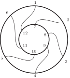
Since , we have both
and
only when is even; see Figure
5. Thus
(34)
For odd we write . Then
This shows that condition (ii) of
Definition 25 is
satisfied.
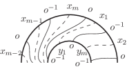
Figure 5. When the only spoke diagrams that make a contribution
are those where we connect an to an . This
means we can only connect an to a if the indices
have the same parity. This is what we see in equation
(34).
∎
Definition 53.
A random matrix is said to be invariant under conjugation by
an orthogonal matrix if the joint distribution of the
entries is invariant under conjugation by an orthogonal
matrix. So if we let be a random matrix, be a
orthogonal matrix and then we mean that for
every we have
Many standard examples of random matrices are invariant
under conjugation by a unitary or orthogonal matrix. In
particular, real Wishart matrices, the Gaussian orthogonal
ensemble, Ginibre matrices, and orthogonal matrices are all
invariant under conjugation by an orthogonal matrix. In
[r1, r2], Redelmeier these were shown to have real second
order limit distributions and so satisfy the hypothesis of
our theorem below.
Theorem 54.
Suppose that and are two
independent families of random matrices, each with real
second order limit distribution. Suppose also that the
family is invariant under conjugation by an
orthogonal matrix. Then and
are asymptotically real second order free.
Proof.
Since the joint distribution of the entries of and
are the same we may replace by
and then apply
Proposition 52.
∎
10. Concluding Remark
Let us consider and two
independent ensembles of random matrices, each with a real
second order limit distribution and suppose that the
ensemble is invariant under a conjugation by
a unitary matrix. In [mśs] it is shown that and are asymptotically complex
second order free (see [mśs], Corollary 3.16). Since
orthogonal matrices are also unitary, Theorem
54 implies that and
are asymptotically both real and
complex second order free. In particular, the second term on
the right-hand side of equation
(6) must vanish. In
consequence, for we have that
The connection between ensembles of random matrices which
are invariant under a conjugation with a unitary and real
second order freeness goes deeper than this and is
investigated in the subsequent paper [mp2] in which we show that unitarily invariant ensembles are asymptotically free from their transposes.
References
[agz] G. Anderson, A. Guionnet, and
O. Zeitouni, An introduction to random matrices,
Cambridge University Press, 2010.
[az] G. Anderson and O. Zeitouni, A CLT
for a band matrix model, Probab. Theory Related
Fields134 (2006), 283-338.
[bs] Z. D. Bai and J. W. Silverstein, CLT
for linear spectral statistics of large-dimensional sample
covariance matrices. Ann. Probab.32
(2004), 553-605.
[c] B. Collins: Moments and
cumulants of polynomial random variables on unitary
groups, the Itzykson-Zuber integral, and free
probability. Int. Math. Res. Not.,
(17) (2003), 953-982.
[cmśs] B. Collins, J. A. Mingo,
P. Śniady, and R. Speicher, Second Order
Freeness and Fluctuations of Random Matrices:
III. Higher Order Freeness and Free Cumulants,
Documenta Math., 12 (2007), 1-70.
[cs] B. Collins and P. Śniady,
Integration with Respect to the Haar Measure on Unitary,
Orthogonal, and Symplectic Group,
Comm. Math. Phy., 264 (2006), 773-795.
[fmp] J. B. French, P. A. Mello, and
A. Pandey, Statistical properties of many-particle
spectra. II. Two-point correlations and
fluctuations. Ann. Physics113 (1978),
277-293.
[j] K. Johansson, On fluctuations of
eigenvalues of random Hermitian matrices, Duke
Math. J., 91 (1998), 151-204.
[k] C. King. Two-dimensional Potts models
and annular partitions, J. Statist. Phy., 96 (1999), 1071–1089.
[kkp] A. Khorunzhy, B. Khoruzhenko, and
L. Pastur, On the corrections to the Green functions
of random matrices with independent
entries. J. Phys. A28 (1995), L31-L35.
[lz] S. K. Lando and A. K. Zvonkin,
Graphs on surfaces and their applications,
Springer-Verlag, 2004.
[ls] V. P. Leonov and A. N. Shiryaev, On a method of
semi-invariants, Theory of Probability and its
Applications, 4 (1959), 319–329.
[mp1] V. A. Marčenko and
L. A. Pastur, Distribution of eigenvalues in certain sets
of random matrices, (Russian) Mat. Sb. (N.S.)72 (114) (1967), 507 536.
[mn] J. A. Mingo and A. Nica, Annular
noncrossing permutations and partitions, and second-order
asymptotics for random matrices,
Int. Math. Res. Not., 28 (2004),
1413-1460.
[mp2] J. A. Mingo, M. Popa, On the
Relation between the Complex and Real Second order Free
Independence, preprint.
[ms] J. A. Mingo and R. Speicher:
Second Order Freeness and Fluctuations of
Random Matrices: I. Gaussian and Wishart matrices and
Cyclic Fock spaces. J. Funct. Anal.,
235, (2006), 226-270.
[mśs] J. A. Mingo, P. Śniady, and
R. Speicher, Second order freeness and fluctuations of
random matrices: II. Unitary random matrices.
Adv. in Math.209 (2007), 212-240.
[mst] J. A. Mingo, R. Speicher, and
E. Tan, Second Order Cumulants of Products,
Trans. Amer. Math. Soc., 361, (2009),
4751-4781.
[ns] A. Nica and R. Speicher,
Lectures on the Combinatorics of Free
Probability, Cambridge Univ. Press, 2006.
[r1] C. E. I. Redelmeier, Genus
expansion for real Wishart matrices,
J. Theoret. Probab.24 (2011),
1044-1062.
[r2] C. E. I. Redelmeier, Real
second-order freeness and the asymptotic real second-order
freeness of several real matrix ensembles,
I.M.R.N. (to appear).
[s] R. Speicher: Multiplicative
functions on the lattice of noncrossing partitions and
free convolution. Math. Ann.,
298 (1994), 611-628.
[v1] D.-V. Voiculescu, Limit laws for
random matrices and free products, Invent. Math.104 (1991), 201-220.
[v2] D.-V. Voiculescu, A strengthened
asymptotic freeness result for random matrices with
applications to free entropy,
Internat. Math. Res. Notices, 1998, no. 1, 41-63.
[vdn] D. V. Voiculescu, K. Dykema, and
A. Nica, Free Random variables, Amer. Math. Soc.,
1992.
[w] E. P. Wigner, Characteristic vectors of
bordered matrices with infinite dimensions,
Ann. of Math.62 (1955), 548 564.