The AG-invariant for $(m+2)$-angulations

Abstract.

In this paper, we study gentle algebras that come from $(m+2)$-angulations of unpunctured Riemann surfaces with boundary and marked points. We focus on calculating a derived invariant introduced by Avella-Alaminos and Geiss, generalizing previous work done when $m=1$. In particular, we provide a method for calculating this invariant based on the the configuration of the arcs in the $(m+2)$-angulation, the marked points, and the boundary components.

1. Introduction

The derived equivalence classes of $m$-cluster-tilted algebras of type $\mathbb{A}$ were determined in [15] using the cycles with full relations in the bound quiver $(Q,I)$ as an invariant. Recently, in [10], the Hochschild cohomology and an invariant of Avella-Alaminos and Geiss [4], the AG-invariant, were used to describe all connected algebras derived equivalent to a connected component of an $m$-cluster-tilted algebra of type $\mathbb{A}$. Given an algebra $\Lambda$, both [10, 15] make use of a normal form $N_{r,s}$ associated to the bound quiver $(Q,I)$ of $\Lambda$. In particular, [10] calculates the AG-invariant of $\Lambda$ using the normal form quiver $N_{r,s}$. This method generalizes the method for calculating the AG-invariant for the iterated tilted algebras of type $\mathbb{A}$ given in [12]. We will make use of the description of $m$-cluster-tilted algebra as arising from the $(m+2)$-angulation of an $(n+1)m+2$-gon $(P,M,T)$.

To state the main theorem we need to define certain sets. Call $M$ the set of marked points, one for each vertex of the polygon $P$. The set $T$ is the collection of diagonals in the $(m+2)$-angulation. We identify are particular subset $M_{T}$ if $M$ consisting of those marked points incident to at least one diagonal in $T$. Denote by $\mathfrak{B}$ the set of boundary segments $\mathfrak{b}$ which are demarcated by the elements in $M_{T}$. Finally, set

$$(a,b)^{*}=f(x,y)=\begin{cases}1&(x,y)=(a,b),\\ 0&\text{ otherwise}.\end{cases}$$

Theorem.

Let $\Lambda$ be a connected algebra associated to the $(m+2)$-angulation $(P,M,T)$. The AG-invariant of $\Lambda$ is the function $(a,b)^{*}+t(0,m+2)^{*}$ where

$$a=\#M_{T},\quad\text{and}\quad b=\sum_{\mathfrak{B}}(m-w(\mathfrak{b}_{i}))$$

with $w(\mathfrak{b}_{i})=\#(\mathfrak{b}_{i}\cap M\setminus M_{T})$ and $t$ is the number of internal $(m+2)$-gons in $(P,M,T)$.

When $m=1$, this calculation recovers Theorem 4.6 from [12]. Additionally, in [12] a class of algebras called surface algebras is introduced via a process called admissible cutting of the surface. When the surface is a disc (that is, when we consider a triangulation of a polygon) this construction produces the iterated tilted algebras of type $\mathbb{A}$ with global dimension 2. We will show how to realize these algebras as $m$-cluster-tilted algebras of type $\mathbb{A}$. This realization agrees with Corollary 6.6 in [10].

After considering the disc the next step is to consider those surfaces with multiple boundary components. When considering triangulations, the immediate benefit is that cluster-tilted algebras of affine type $\widetilde{\mathbb{A}}$ arise as triangulations of the annulus. In [12], the calculation of the AG-invariant is done for any surface with any number of boundary components. Similarly, we extend the main theorem to those surfaces with more than one boundary component. This work also shows how to deal with $(m+2)$-angulations that are are not connected.

To calculate the AG-invariant for arbitrary $(m+2)$-angulations $(P,M,T)$, we introduce the concept of boundary bridges in section 5. We then define a new $(m+2)$-angulation $(\widetilde{P},\widetilde{M},\widetilde{T})$ by removing these boundary bridges. This operation does not disturb the arcs in $T$, so $(Q_{\widetilde{T}},I_{\widetilde{T}})=(Q_{T},I_{T})$. Using this new surface we can calculate the AG-invariant as before.

Theorem.

Let $(P,M,T)$ be any $(m+2)$-angulation and $\Lambda$ the corresponding algebra. The AG-invariant of $\Lambda$ is given by

$$t(0,m+2)^{*}+\sum_{i}(a_{i},b_{i})^{*}$$

where $t$ is number of internal $(m+2)$-gons in $(P,M,T)$, $i$ indexes the boundary components of $\widetilde{P}$, and

$$a_{i}=\#\widetilde{M}_{T}^{i},\quad\text{and}\quad b_{i}=\sum_{\mathfrak{b}_{j}\in\widetilde{\mathfrak{B}}_{i}}(m-w(\mathfrak{b}_{j})).$$

In this theorem $\widetilde{M}_{T}^{i}$ and $\mathfrak{B}_{i}$ are defined as before but restricted to the $i$th boundary component. Note that if there are no boundary bridges in $(P,M,T)$, then we set $(\widetilde{P},\widetilde{M},\widetilde{T})=(P,M,T)$.

2. Preliminaries

2.1. Gentle algebras

Let $k$ be an algebraically closed field. Recall from [3] that a finite-dimensional algebra $\Lambda$ is gentle if it admits a presentation $\Lambda=kQ/I$ satisfying the following conditions:

• At each point of $Q$ there starts at most two arrows and stops at most two arrows.

• The ideal $I$ is generated by paths of length 2.

• For each arrow $\beta$ there is at most one arrow $\alpha$ and at most one arrow $\gamma$ such that $\alpha\beta\in I$ and $\beta\gamma\in I$.

• For each arrow $\beta$ there is at most one arrow $\alpha$ and at most one arrow $\gamma$ such that $\alpha\beta\not\in I$ and $\beta\gamma\not\in I$.

An algebra $\Lambda=kQ/I$ where $I$ is generated by paths and $(Q,I)$ satisfies the two conditions (G1) and (G4) is called a string algebra (see [11]), thus every gentle algebra is a string algebra.

2.2. The AG-invariant

We recall from [4] the definition of the derived invariant of Avella-Alaminos and Geiss. From this point on called the AG-invariant. Let $\Lambda$ be a gentle $k$-algebra with bound quiver $(Q,I)$, $Q=(Q_{0},Q_{1},s,t)$ where $s,t\colon Q_{1}\to Q_{0}$ are the source and target functions on the arrows.

Definition 1.

A permitted path of $\Lambda$ is a path $H=\alpha_{1}\alpha_{2}\cdots\alpha_{n}$ in $Q$ which is not in $I$. We say a permitted path is a non-trivial permitted thread of $\Lambda$ if for all arrows $\beta\in Q_{1}$, neither $\beta H$ nor $H\beta$ is a permitted path. These are the ‘maximal’ permitted paths of $\Lambda$. Dual to this, we define the forbidden paths of $\Lambda$ to be a sequence $F=\alpha_{1}\alpha_{2}\cdots\alpha_{n}$ in $Q$ such that $\alpha_{i}\neq\alpha_{j}$ unless $i=j$, and $\alpha_{i}\alpha_{i+1}\in I$, for $i=1,\dots,n-1$. A forbidden path $F$ is a non-trivial forbidden thread if for all $\beta\in Q_{1}$, neither $\beta F$ or $F\beta$ is a forbidden path. We also require trivial permitted and trivial forbidden threads. Let $x\in Q_{0}$ such that there is at most one arrow starting at $x$ and at most one arrow ending at $x$. Then the constant path $e_{x}$ is a trivial permitted thread if when there are arrows $\beta,\gamma\in Q_{1}$ such that $s(\gamma)=x=t(\beta)$, then $\beta\gamma\not\in I$. Similarly, $e_{x}$ is a trivial forbidden thread if when there are arrows $\beta,\gamma\in Q_{1}$ such that $s(\gamma)=x=t(\beta)$, then $\beta\gamma\in I$.

Let $\mathcal{H}$ denote the set of all permitted threads and $\mathcal{F}$ denote the set of all forbidden threads.

Notice that each arrow in $Q_{1}$ is both a permitted and a forbidden path. Moreover, the constant path at each sink and at each source will simultaneously satisfy the definition for a permitted and a forbidden thread because there are no paths going through $x$.

We fix a choice of functions $\sigma,\varepsilon\colon Q_{1}\to\{-1,1\}$ characterized by the following conditions.

1. If $\alpha_{1}\neq\alpha_{2}$ are arrows with $s(\alpha_{1})=s(\alpha_{2})$, then $\sigma(\alpha_{1})=-\sigma(\alpha_{2})$.

2. If $\alpha_{1}\neq\alpha_{2}$ are arrows with $t(\alpha_{1})=t(\alpha_{2})$, then $\varepsilon(\alpha_{1})=-\varepsilon(\alpha_{2})$.

3. If $\alpha,\beta$ are arrows with $s(\beta)=t(\alpha)$ and $\alpha\beta\not\in I$, then $\sigma(\beta)=-\varepsilon(\alpha)$.

Note that the functions need not be unique. Given a pair $\sigma$ and $\varepsilon$, we can define another pair $\sigma^{\prime}:=-1\sigma$ and $\varepsilon^{\prime}:=-1\varepsilon$.

These functions naturally extend to paths in $Q$. Let $\Pi=\alpha_{1}\alpha_{2}\cdots\alpha_{n-1}\alpha_{n}$ be a path. Then $\sigma(\Pi)=\sigma(\alpha_{1})$ and $\varepsilon(\Pi)=\varepsilon(\alpha_{n})$. We can also extend these functions to trivial threads. Let $x,y$ be vertices in $Q_{0}$, $h_{x}$ the trivial permitted thread at $x$, and $p_{y}$ the trivial forbidden thread at $y$. Then we set

$$\sigma(h_{x})=-\varepsilon(h_{x}) =-\sigma(\alpha), s(\alpha)=x,\text{ or}$$ if

$$\sigma(h_{x})=-\varepsilon(h_{x}) =-\varepsilon(\beta), t(\beta)=x$$ if

and

$$\sigma(p_{y})=\varepsilon(p_{y}) =-\sigma(\gamma), s(\gamma)=y,\text{ or}$$ if

$$\sigma(p_{y})=\varepsilon(p_{y}) =-\varepsilon(\delta), t(\delta)=y,$$ if

where $\alpha,\beta,\gamma,\delta\in Q_{1}$. Recall that these arrows are unique if they exist.

Definition 2.

The AG-invariant $\operatorname{AG}(\Lambda)$ is defined to be a function depending on the ordered pairs generated by the following algorithm.

1. 1. Begin with a permitted thread of $\Lambda$, call it $H_{0}$.

   2. To $H_{i}$ we associate $F_{i}$, the forbidden thread which ends at $t(H_{i})$ and such that $\varepsilon(H_{i})=-\varepsilon(F_{i})$. Define $\varphi(H_{i}):=F_{i}$.

   3. To $F_{i}$ we associate $H_{i+1}$, the permitted thread which starts at $s(F_{i})$ and such that $\sigma(F_{i})=-\sigma(H_{i+1})$. Define $\psi(F_{i}):=H_{i+1}$.

   4. Stop when $H_{n}=H_{0}$ for some natural number $n$. Define $m=\sum_{i=1}^{n}\ell(F_{i})$, where $\ell(C)$ is the length (number of arrows) of a path $C$. In this way we obtain the pair $(n,m)$.

2. Repeat (1) until all permitted threads of $A$ have occurred.

3. For each oriented cycle in which each pair of consecutive arrows form a relation, we associate the ordered pair $(0,n)$, where $n$ is the length of the cycle.

We define $\operatorname{AG}(\Lambda)\colon\mathbb{N}^{2}\to\mathbb{N}$ where $\operatorname{AG}(\Lambda)(n,m)$ is the number of times the ordered pair $(n,m)$ is formed by the above algorithm.

Example 3.

Let $(Q,I)$ be the following quiver:

where $I=\langle\alpha_{3}\alpha_{5},\alpha_{4}\alpha_{2}\rangle$. Then the permitted threads are

$$\mathcal{H}=\{\alpha_{2}\alpha_{1}\alpha_{3}\alpha_{4},\alpha_{5},e_{1},e_{3},e_{5}\}$$

and the forbidden threads are

$$\mathcal{F}=\{\alpha_{4}\alpha_{2},\alpha_{3}\alpha_{5},\alpha_{1},e_{2},e_{5}\}.$$

Notice that $e_{5}$ is both a permitted and forbidden trivial thread. When necessary, we will use the notation $h_{x}$ and $p_{x}$ to distinguish when we consider $e_{x}$ a permitted or forbidden thread respectively.

We can define the functions $\sigma$ and $\varepsilon$ such that on the threads of $(Q,I)$ we have:

$$\mathcal{H}$$

                 

                 

Then the calculation of the AG-invariant is given in the following tables:

$$H_{i}$$

0

1

2

3

4

                 

0

1

In this case we have

$$\operatorname{AG}(\Lambda)(n,m)=(1,0)^{*}+(4,5)^{*}=\begin{cases}1\text{; if }(n,m)=(1,0)\text{ or }(4,5),\\ 0\text{; otherwise}.\end{cases}$$

The algorithm defining $\operatorname{AG}(\Lambda)$ can be thought of as dictating a walk in the quiver $Q$, where we move forward on permitted threads and backward on forbidden threads, see [4].

Remark 4.

Note that the steps (1b) and (1c) of this algorithm give two different bijections $\varphi$ and $\psi$ between the set of permitted threads $\mathcal{H}$ and the set of forbidden threads which do not start and end in the same vertex. We will often refer to the permitted (respectively forbidden) thread “corresponding” to a given forbidden (respectively permitted) thread. This correspondence is referring to the bijection $\varphi$ (respectively $\psi$).

2.3. $m$-cluster-tilted algebras

Cluster categories were introduced in [8]. Quickly after, the notion of cluster-tilted algebras were introduced and studied in [1, 2, 6, 7] to name only a few. This construction was then generalized to $m$-cluster categories and $m$-cluster-titled algebras in [16, 14, 13] among others. Roughly, the $m$-cluster category is defined as the orbit category $\mathcal{D}^{b}(\operatorname{mod}kQ)/\langle\tau^{-1}[m]\rangle$ where $Q$ is an acyclic quiver. The $m$-cluster-tilted algebras are then defined as the endomorphism algebras of tilting objects in this category. For a complete description of this development we recommend [13, 16]. We focus on the combinatorial description of $m$-cluster categories and the corresponding $m$-cluster-tilted algebras given via $(m+2)$-angulations which has been studied in [5, 9, 15], we will generally adapt the definitions found in [15].

Let $P$ be a disc with boundary and $M$ be a finite set contained in $\partial P$. Note that $(P,M)$ is equivalent to a polygon with $\#M$ edges. It is common to simply take a polygon, but we prefer the generality of the language of a surface with marked points.

Definition 5.

An $m$-allowable diagonal in $(P,M)$ is a chord joining two non-adjacent points in $M$ such that $(P,M)$ is divided into two smaller polygons $P_{1}$ and $P_{2}$ which can themselves be divided into $(m+2)$-gons by non-crossing chords.

Definition 6.

The collection $(P,M,T)$ is called an $(m+2)$-angulation of $(P,M)$ if $T$ is a maximal collection of $m$-allowable diagonals. We denote a $(m+2)$-gon in $(P,M,T)$ by $\triangle$.

In [15], it is a simple lemma that $(P,M)$ can be divided into an $(m+2)$-angulation if and only if $\#M\equiv 2\operatorname{mod}m$.

Definition 7.

To a $(m+2)$-angulation $(P,M,T)$ we associate a quiver with relations $(Q_{T},I_{T})$. The vertices of $Q_{T}$ are in bijection with the elements of $T$. For any two vertices $x$ and $y$ in $Q_{T}$ we have an arrow $x\to y$ if and only if:

1. the corresponding $m$-allowable diagonals $\tau_{x}$ and $\tau_{y}$ share a vertex in $(P,M)$,

2. $\tau_{x}$ and $\tau_{y}$ are edges of the same $(m+2)$-gon $\triangle$ in the $(P,M,T)$,

3. $\tau_{y}$ follows $\tau_{x}$ in the counter-clockwise direction (as you walk around the boundary of $\triangle$).

Example 8.

The quiver associated to the $(m+2)$-angulation given in Figure 1 is

$$1\xrightarrow{\ \ \alpha_{1}\ \ }2\xrightarrow{\ \ \alpha_{2}\ \ }3\xleftarrow{\ \ \alpha_{3}\ \ }4\xleftarrow{\ \ \alpha_{4}\ \ }5\xrightarrow{\ \ \alpha_{5}\ \ }6\xrightarrow{\ \ \alpha_{6}\ \ }7$$

with $I_{T}=\langle\alpha_{1}\alpha_{2},\alpha_{5}\alpha_{6}\rangle$.

In much of the literature, people choose either the counter-clockwise orientation or the clockwise orientation. The choice does not affect the final results of the theory but should be carefully noted when doing calculations, choosing to use the clockwise orientation will produce $Q_{T}^{\mathrm{op}}$. Some of the lemmas in the following section will depend on this choice of direction but can easily be restated in the clockwise direction.

3. Calculating the AG-invariant

Definition 9.

Let $\Lambda$ be the $m$-cluster-tilted algebra associated to the $(m+2)$-angulation $(P,M,T)$. Let

$$M_{T}:=\{p\in M:p\text{ is incident to }T\},$$

and

$$\mathfrak{B}=\{\mathfrak{b}_{1},\dots,\mathfrak{b}_{r}\}$$

be the pieces of the boundary component such that the endpoints of $\mathfrak{b}_{i}$ are in $M_{T}$ and each $\mathfrak{b}_{i}$ does not contain any other points of $M_{T}$. Further, let $w(\mathfrak{b}_{i})$ be the number of marked points on $\mathfrak{b}_{i}$ not contained in $M_{T}$. That is

$$w(\mathfrak{b}_{i})=\#((M\cap\mathfrak{b}_{i})\setminus M_{T}).$$

Example 10.

In Figure 1 the set $M_{T}$ is given by the white marked points.

Figure 1. The white points indicate elements of $M_{T}$. The boundary segments have weights $w(\mathfrak{b}_{1})=w(\mathfrak{b}_{2})=w(\mathfrak{b}_{5})=w(\mathfrak{b}_{6})=2$, $w(\mathfrak{b}_{3})=w(\mathfrak{b}_{4})=1$, and $w(\mathfrak{b}_{7})=w(\mathfrak{b}_{8})=0$.

Lemma 11.

Let $\Lambda$ be the algebra associated to the $(m+2)$-angulation $(P,M,T)$. The permitted threads of $\Lambda$ are in bijection with $M_{T}$

Proof.

This follows from the definition of $Q_{T}$. By construction, the arrows of $Q_{T}$ are given by the angles of the $(m+2)$-gons in $(P,M,T)$, further arrows $\alpha$ and $\beta$ are composable if and only if the angles defining $\alpha$ and $\beta$ are incident to each other at the same marked point. It follows that to any permitted thread we can associate a marked point in $M_{T}$. Conversely, given a marked point in $p\in M_{T}$, we can associate a sequence of arrows $H$ defined by the angles incident to $p$. This sequence must define a permitted thread, since any other arrows that we may consider to compose with $H$ must come from angles not incident to $p$. Hence the composition is zero by the definition of $I_{T}$. Notice that the trivial forbidden threads are given by marked points incident to a unique edge in $T$. ∎

Example 12.

Applying Lemma 11 to Figure 1 and using the labels on the corresponding quiver given in Example 8 we get the following list of permitted threads written in counter-clockwise order based on the corresponding marked point:

$$\alpha_{4}\alpha_{3},e_{1},\alpha_{1},\alpha_{2},e_{4},\alpha_{5},\alpha_{6},e_{7}.$$

Lemma 13.

Let $\Lambda$ be the algebra associated to the connected $(m+2)$-angulation $(P,M,T)$. The forbidden threads of $\Lambda$ are in bijection with $\mathfrak{B}$. Further, if $F\in\mathcal{F}$ is associated to $\mathfrak{b}_{i}\in\mathfrak{B}$, then $\ell(F)=m-w(\mathfrak{b}_{i})$.

Proof.

This proof is similar to the proof of Lemma 11. By the definition of $I_{T}$, the composition $\alpha\beta\in I_{T}$ if and only if $\alpha$ and $\beta$ are defined by neighboring angles of the same $(m+2)$-gon. Hence, the forbidden threads can be identified with the $(m+2)$-gons of $(P,M,T)$. Additionally, by assumption the $(m+2)$-angulation is connected, hence each non-internal $(m+2)$-gon contains exactly one segment from $\mathfrak{B}$, giving us the identification with elements of $\mathfrak{B}$. We do not include the interior $(m+2)$-gons because these, by definition, give rise to an oriented cycle of relations, hence there is no terminal arrow to define the thread.

Similarly, it is clear from the definition of $I_{T}$ that, given an $(m+2)$-gon $\triangle$ bounded by some $\mathfrak{b}$, the composition of the arrows defined in $\triangle$ defines a forbidden thread.

Note that this correspondence also holds for trivial forbidden threads, these threads correspond to $(m+2)$-gons which contain exactly two points from $M_{T}$. Such a $(m+2)$-gon contains a single edge of $T$, say $\tau_{i}$, which corresponds to a source, a sink, or the intermediate vertex of a relation in $I_{T}$. In each of these cases $e_{i}$ is a trivial forbidden thread.

Let $F$ be a forbidden thread, $\triangle$ the corresponding $(m+2)$-gon, and $\mathfrak{b}$ the corresponding edge from $\mathfrak{B}$. From the first paragraph, we immediately see that $\ell(F)$ is the number of angles in $\triangle$ constructed from edges in $T$. We wish to count these angles. There are $(m+2)$ total angles in $\triangle$ coming in three types: $\ell(F)$ many angles completely constructed by $T$, $w(\mathfrak{b})$ many completely constructed by $\mathfrak{b}$, and the two angles where $T$ and $\mathfrak{b}$ meet. Hence, we have $m+2=\ell(F)+w(\mathfrak{b})+2$ and we immediately see $\ell(F)=m-w(\mathfrak{b})$, as desired. ∎

Recall from Remark 4, the steps (1b) and (1c) of the AG algorithm give two different bijections $\varphi$ and $\psi$ between the set of permitted threads $\mathcal{H}$ and the set of forbidden threads which do not start and end in the same vertex. Throughout the proofs of the following lemmas we will use $p\in M_{T}$ and $\mathfrak{b}\in\mathfrak{B}$ to both represent the elements of each respective set but also the corresponding permitted or forbidden thread in $(Q_{T},I_{T})$.

Lemma 14.

Let $p\in M_{T}$ and let $p$ also denote the corresponding permitted thread, then the forbidden thread $\varphi(p)$ is given by the edge $\mathfrak{b}\in\mathfrak{B}$ incident to and following $p$ in the counter-clockwise direction.

Proof.

The sequence of edges incident to $p$ can end in two ways: (1) bounding an $(m+2)$-gon $\triangle$ incident to exactly two points of $M_{T}$ or (2) bounding $\triangle$ which is incident to more than two points of of $M_{T}$. In both cases, $\triangle$ contains a boundary segment from $\mathfrak{B}$, let $\mathfrak{b}$ be this segment. In the first case, the boundary segment $\mathfrak{b}$ corresponds to a trivial forbidden thread, we have one of the following figures:

      or            or      

corresponding to a sink, source or neither in $Q_{T}$. In the first figure there are two forbidden threads $\mathfrak{b}$ and $\mathfrak{b}^{\prime}$ ending at $t(p)$. By the definition of $\varepsilon$ we must have $\varepsilon(\mathfrak{b}^{\prime})=\varepsilon(p)$ because $\mathfrak{b}$ corresponds to the final arrow of $p$. Similarly, $\varepsilon(\mathfrak{b})=-\varepsilon(p)$, hence $\varphi(p)=\mathfrak{b}$. In the last two cases the only possible forbidden thread ending at $t(p)$ is $\mathfrak{b}$. It is a simple check that $\mathfrak{b}$ must satisfy the compatibility condition on $\varepsilon$ used in step 1(b) defining the AG-invariant. It follows that $\varphi(p)=\mathfrak{b}$.

If the ending $(m+2)$-gon $\triangle$ is of type (2), that is, if $\triangle$ contains more that two points of $M_{T}$, then there is a unique choice for the forbidden thread $\varphi(p)$. We have the following figure

      or      

where we $\widetilde{\tau}$ the other required edges of $\triangle$. We allow that $\widetilde{\tau}$ does not exist, so $w(\mathfrak{b})=m-1$. If $p$ is a trivial thread, then the only forbidden thread ending at $\tau_{x}$ is $\mathfrak{b}$ and it follows immediately that $\varepsilon(p)=-\varepsilon(\mathfrak{b})$ as required. On the other hand if $p$ is not trivial, then the final arrow $\alpha$ of the thread $p$ is also a forbidden thread (of length 1). Let $\beta$ denote the final arrow of $\mathfrak{b}$, which is formed by the angle between $\tau_{y}$ and $\tau_{x}$. From the definition of $\varepsilon$, we must have $\varepsilon(p)=\varepsilon(\alpha)=-\varepsilon(\beta)=-\varepsilon(\beta)$, as desired. Hence $\varphi(p)=\mathfrak{b}$. ∎

Lemma 15.

Let $\mathfrak{b}\in\mathfrak{B}$ and let $\mathfrak{b}$ also denote the corresponding forbidden thread, then the permitted thread $\psi(\mathfrak{b})$ is the marked point $p\in M_{T}$ incident to and following $\mathfrak{b}$ in the counter-clockwise direction.

Proof.

Let $p$ be as in the statement, further let $\tau$ be the edge incident to $p$ and bounding the $(m+2)$-gon containing $\mathfrak{b}$.

As in the previous lemma, we consider two cases. First assume that $w(\mathfrak{b})=m$, so that $\mathfrak{b}$ is a trivial forbidden thread, call the corresponding vertex corresponds to $\tau$. This has two sub-cases. If $\tau$ is not the source of any arrows, then $p$ is the trivial permitted thread at $\tau$ and the definition of $\sigma$ immediately implies that $\sigma(\mathfrak{b})=-\sigma(p)$, hence $\psi(\mathfrak{b})=p$. The second sub-case, if $x$ is the source of an arrow, this arrow must be unique and formed by an angle incident to $p$. Call this arrow $\alpha$, we must have $\sigma(p)=\sigma(\alpha)=-\sigma(\mathfrak{b})$.

Now assume that $w(\mathfrak{b})<m$, so $\mathfrak{b}$ is a non-trivial forbidden thread. Let $\beta$ denote the initial arrow of this thread, note that $s(\beta)=\tau$. In this case, $p$ may represent either a trivial or a non-trivial permitted thread. In both cases, we have $\sigma(\mathfrak{b})=\sigma(\beta)=-\sigma(p)$, hence $\psi(\mathfrak{b})=p$. ∎

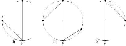
Figure 2. Possible configurations for $\tau$ in Lemma 15.

Theorem 16.

Let $\Lambda$ be the algebra associated to the connected $(m+2)$-angulation $(P,M,T)$. The AG-invariant of $\Lambda$ is $(a,b)^{*}+t(0,m+2)^{*}$ where $t$ is number of internal $(m+2)$-gons in $(P,M,T)$ and

$$a=\#M_{T},\quad\text{and}\quad b=\sum_{\mathfrak{B}}(m-w(\mathfrak{b}_{i})).$$

Proof.

This follows immediately from Lemma 11, 13, 14, and 15 and the definition of the AG algorithm. ∎

4. Surface algebras as $m$-cluster-tilted

For brevity we omit the definition of surface algebras given in [12], hence, we will not discuss the concept of admissible cuts, instead, we define surface algebras as algebras arising from particular partial triangulations of surfaces. Further, we will focus on the case when the surface is a disc. The resulting algebra is iterated tilted of type $\mathbb{A}_{n}$ with global dimension at most 2. The definition we give could easily be extended to other type, but it will not be needed.

Definition 17.

Let $(P,M)$ be a disc with marked points in the boundary. Fix a partial triangulation $T$ such that the non-triangular components are squares containing exactly one edge in the boundary. As for $(m+2)$-angulations, we define the bound quiver $(Q_{T},I_{T})$ where $(Q_{T})_{0}$ is indexed by the edges in $T$ and there is an arrow $\alpha\colon i\to j$ if $\tau_{i}$ and $\tau_{j}$ form an angle in a triangle (or square) in $T$ and $j$ follows $i$ in the counter-clockwise direction. As before, we say the arrow $\alpha$ lives in the triangle (resp. square) that $\tau_{i}$ and $\tau_{j}$ bound. We can then define the ideal $I_{T}$ by setting $\alpha\beta\in I_{T}$ if $\alpha$ and $\beta$ live in the same square.

Example 18.

The quiver associated to the partial triangulation given in Figure 3 is

$$1\xleftarrow{\ \ \alpha_{1}\ \ }2\xrightarrow{\ \ \alpha_{2}\ \ }3\xrightarrow{\ \ \alpha_{3}\ \ }4$$

with $I_{T}=\langle\alpha_{2}\alpha_{3}\rangle$.

Figure 3. A partial triangulation of the disc.

Given an iterated tilted algebra $\Lambda$ of type $\mathbb{A}$ defined via a partial triangulation, we will show that $\Lambda$ is $m$-cluster-tilted for any $m>1$ by realizing it as an $(m+2)$-angulation of the disc. Further, the calculation of the AG-invariant independent of the choice of $m$.

Let $(P,M,T)$ be the partial triangulation of $\Lambda$ and define the sets $M_{T}$ and $\mathfrak{B}$ as in section 3. For $m>1$, we construct a $(m+2)$-angulation from $(P,M,T)$ as follows. To each edge $\mathfrak{b}\in\mathfrak{B}$ we add the following number of marked points

(1) $$\begin{cases}m-2&\text{if }\mathfrak{b}\text{ bounds a square},\\ m-1&\text{otherwise}.\\ \end{cases}$$

let $M^{\prime}$ be the new marked points, we define an $(m+2)$-angulation $(P,M\cup M^{\prime},T)$ where $(P,M,T)$ is the original partial triangulation. Because we are not creating any new edges or angles, the quiver of $(P,M\cup M^{\prime},T)$ is exactly the quiver $Q_{T}$ associated to $(P,M,T)$. Notice that the total number of points for each component polygon of $T$ will be $4+m-2=m+2$ or $3+m-1=m+2$, hence this process does indeed produce an $(m+2)$-angulation. Further, by the construction of $(Q_{T},I_{T})$, it immediately follows from the definition given in [15] that $\Lambda$ is $m$-cluster-tilted of type $\mathbb{A}_{n}$.

We note that recent work in [13] has shown how to construct $m$-cluster-tilted algebras from iterated tilted algebras with global dimension at most $m+1$ via relation extensions, extending work that was done for $m=1$ in [2]. The realization we have constructed above will only create $m$-cluster-tilted algebras with global dimension at most 2. It should also be remarked the that above construction verifies a special case of Corollary 6.6(b) in [10]. We formalize the above discussion in the following theorem.

Theorem 19.

The iterated tilted algebras of type $\mathbb{A}$ with global dimension at most 2 are $m$-cluster-tilted algebras for $m>1$.

Example 20.

In Example 18 we associated the following quiver to the partial triangulation given in Figure 3

$$1\xleftarrow{\ \ \alpha_{1}\ \ }2\xrightarrow{\ \ \alpha_{2}\ \ }3\xrightarrow{\ \ \alpha_{3}\ \ }4$$

with $I_{T}=\langle\alpha_{2}\alpha_{3}\rangle$. This quiver also corresponds to the $3+2$-angulation given in Figure 4 which is constructed using equation (1).

Figure 4. The $m=3$ version of Figure 3. The new marked points determined by equation (1) are white.

5. Other surfaces

We begin with an example to demonstrate that the above work can not directly generalize to other surfaces. In the previous sections we have restricted our work to $P$ a disc, we now consider the annulus. When $m=1$, triangulations of the annulus correspond to cluster-tilted algebras of affine Dynkin type $\widetilde{\mathbb{A}}$, hence this is a natural next step after type $\mathbb{A}$. Consider the following $4$-angulation of the annulus:

We hope that this would correspond to 2-cluster tilted algebra of type $\widetilde{\mathbb{A}}$. If we use same rule as given in Defintion 7, then the corresponding quiver with relations ($Q_{T},I_{T})$ is

$$1\xrightarrow{\ \ \alpha\ \ }2\xrightarrow{\ \ \beta\ \ }3$$

with $I_{T}=\langle\alpha\beta\rangle$. This is an iterated tilted algebra of type $\mathbb{A}_{3}$. Further, we can realize this quiver coming from the following $(2+2)$-angulation of the disc

Applying Theorem 16, tells us that the AG-invariant of $(Q_{T},I_{T})$ is $(4,2)^{*}$. However, in the spirit of extending Theorem 4.6 from [12], in the annulus we should apply the main theorem to both boundary components to produce $(2,2)^{*}+(2,4)^{*}$, clearly the incorrect function.

Let $(P,M,T)$ be an $(m+2)$-angulation of an arbitrary surface $P$ with $M_{T}$ and $\mathfrak{B}$ the sets given in Definition 9. The primary issue with the above example is that the $4$-gon bounded by $\tau_{1}$ and $\tau_{3}$ (but not $\tau_{2}$) contains more than one boundary segment from $\mathfrak{B}$. This $4$-gon encodes information about a sink and a source in the corresponding quiver which are are forbidden threads. In Lemmas 11 and 13 we needed a clear bijection between the boundary components $\mathfrak{B}$ and forbidden threads, this bijection and subsequently the lemmas clearly fails in this case. Even though there are exactly two boundary components and two threads, it is not clear which boundary component should correspond to which thread. It is not hard to see that, for $(m+2)$-angulations of surfaces with an arbitrary number of boundary components, these lemmas will extend to those $(m+2)$-angulations such that each $(m+2)$-gon contains at most one element from $\mathfrak{B}$. In fact, it is also seen that all of Section 3 will extend to these $(m+2)$-angulations. To make this concrete, we introduce the following definitions.

Definition 21.

Let $P$ be a surface with a non-empty boundary with any number of boundary components, $M$ a set of points in the boundary with at least one point in each component, and $T$ a collection of arcs contained in the interior of $P$ with endpoints in $M$. We say that $(P,M,T)$ is a $(m+2)$-angulation if it subdivides the interior of $P$ into $(m+2)$-gons. As in Section 3, we set

$$M_{T}:=\{p\in M:p\text{ is incident to }T\},$$

and

$$\mathfrak{B}=\{\mathfrak{b}_{1},\dots,\mathfrak{b}_{r}\}.$$

the pieces of the boundary such that the endpoints of $\mathfrak{b}_{i}$ are in $M_{T}$ and each $\mathfrak{b}_{i}$ does not contain any other points of $M_{T}$. To distinguish elements in a particular boundary component, $M_{T}^{i}$ is the set of marked points in the $i$th boundary component. Similarly, let $\mathfrak{B}_{i}$ be the elements of $\mathfrak{B}$ from the $i$th boundary component. The weight of a boundary segment, $w(\mathfrak{b})$, is defined as before (see Definition 9).

Definition 22.

Let $(P,M,T)$ be an $(m+2)$-angulation of a surface $P$ (which may have more than one boundary component). We say $(P,M,T)$ is a non-degenerate $(m+2)$-angulation if each $(m+2)$-gon in $(P,M,T)$ contains at most one element of $\mathfrak{B}$. All other $(m+2)$-angulations are called degenerate.

Note that the non-degnerate $(m+2)$-angulations inherently give rise to connected quivers. The definition of degenerate includes the $(m+2)$-angulations which are not connected.

With these definitions, Theorem 16 can immediately be extended as follows.

Theorem 23.

If $(P,M,T)$ is a non-degenerate $(m+2)$-angulation and $\Lambda$ the corresponding algebra, then the AG-invariant of $\Lambda$ is given by

$$t(0,m+2)^{*}+\sum_{i>0}(a_{i},b_{i})^{*}$$

where $t$ is number of internal $(m+2)$-gons in $(P,M,T)$, $i$ indexes the boundary components, and

$$a_{i}=\#M_{T}^{i},\quad\text{and}\quad b_{i}=\sum_{\mathfrak{b}_{j}\in\mathfrak{B}_{i}}(m-w(\mathfrak{b}_{j})).$$

∎

In the remainder of this section we will calculate the AG-invariant for degenerate $(m+2)$-angulations. We will do this by a process we call bridging boundary components. In this process we will introduce new boundary segments connecting distinct boundary components of $P$. This will decrease the number of boundary components but will be defined so that the set $\mathfrak{B}$ is extended in such a way that the bijection of Lemma 13 is true. In general, we are modifying the surface so that the resulting $(m+2)$-angulation is no longer degenerate.

Definition 24.

Let $\triangle$ be an $(m+2)$-gon which is bounded by $\{\mathfrak{b}_{1},\dots,\mathfrak{b}_{s}\}\subset\mathfrak{B}$ with $s>1$ and $\{\mathfrak{t}_{1},\dots,\mathfrak{t}_{r}\}$ the boundary segments of $\triangle$ composed of arcs from $T$ with $\mathfrak{t}_{i}$ incident to $\mathfrak{b}_{i-1}$ and $\mathfrak{b}_{i+1}$ (indices are considered modulo $r$). In the example opening this section, $\mathfrak{t}_{1}=\tau_{1}$ and $\mathfrak{t}_{2}=\tau_{3}$. We define the boundary bridge in $\triangle$ as follows.

1. For each segment $\mathfrak{t}_{i}$, let $\delta_{i}^{\prime}$ and $\delta_{i}^{\prime\prime}$ be two curves on $\mathfrak{b}_{i-1}$ and $\mathfrak{b}_{i+1}$ respectively starting at the endpoints of $\mathfrak{t}_{i}$ and denote by $v_{i}^{\prime}$ and $v_{i}^{\prime\prime}$ their respective endpoints. Moreover, we choose $\delta_{i}^{\prime}$, $\delta_{i}^{\prime\prime}$ short enough such that $v_{i}^{\prime}$ and $v_{i}^{\prime\prime}$ are not in $M$ and no point of $M$ (other than the endpoints of $\mathfrak{t}$) lie on the curves $\delta_{i}^{\prime}$, $\delta_{i}^{\prime\prime}$.

2. Let $\mathfrak{t}_{i}^{\prime}$ denote the arc (up to homotopy) in the interior of $P$ connecting $v_{i}^{\prime}$ and $v_{i}^{\prime\prime}$. This results in a new polygon $\triangle_{i}$ bounded by $\mathfrak{t}_{i}$, $\delta_{i}^{\prime}$, $\delta_{i}^{\prime\prime}$ and $\mathfrak{t}_{i}^{\prime}$.

3. Add the appropriate number of marked points to $\mathfrak{t}_{i}^{\prime}$ so that $\triangle_{i}^{\prime}$ is a $(m+2)$-gon. (Recall that we are assuming that $m>1$, so there is zero or more points that need to be added, we never need to remove points.)

4. We refer to the complement of the $\triangle_{i}^{\prime}$s as the boundary bridge in $\triangle$. Note that this includes the pieces of $\mathfrak{b}_{i}$ not in $\delta_{i}^{\prime}$ and $\delta_{i}^{\prime\prime}$ but does not include the arcs $\mathfrak{t}^{\prime}$.

Remark 25.

Notice that this construction does not affect the set $T$ in any way. In particular, if $\tau_{j}$ and $\tau_{k}$ are incident before creating the boundary bridges, then they are still incident after the bridges are constructed.

Example 26.

Consider the $(4+2)$-angulation of the (genus 0) surface with 4 boundary components in Figure 5. It is not difficult to see that the corresponding algebra this can also be realized from a non-degenerate triangulation of a disc. In this figure, this fact is suggested by by the fact that the boundary bridges connect all of the original boundary components. If we cut out the boundary bridges, there will be a single boundary component. The corresponding triangulation is then created by reducing the number or marked points until each $(m+2)$-gon becomes a triangle. Notice that when we cut out the bridges, two of the original marked points are removed, so this operation while preserving $T$, does not preserve $M$ as a subset of the new marked point set.

Figure 5. The $(4+2)$-angulation is degenerate, with two 6-gons containing boundary bridges. The white marked points are those added while constructing the bridges and the dark red-grey area is the interior of the bridges.

Definition 27.

Let $(P,M,T)$ be a degenerate $(m+2)$-angultion. Define $(\widetilde{P},\widetilde{M},\widetilde{T})$ to be the $(m+2)$-angulation constructed by removing all boundary bridges from $(P,M,T)$. For compactness of notation we use the following convention that $(\widetilde{P},\widetilde{M},\widetilde{T})=(P,M,T)$ when the $(m+2)$-angulation is non-degenerate, in this case there are no boundary bridges and hence nothing to remove.

Notice that if $T$ is connected, then $\widetilde{P}$ will be a connected surface. On the other hand, if $T$ is not connected, then removing the boundary bridges will result in a surface which is not connected. In either case, the removal of the boundary bridges has a significant impact on the number of boundary components and the set $\mathfrak{B}$. Let $\widetilde{\mathfrak{B}}$ denote the set of boundary segments with endpoints in $\widetilde{M}_{T}$, as in Definition 21. The set $\widetilde{\mathfrak{B}}$ consists of the segments in $\mathfrak{B}$ plus the segments $\delta_{i}^{\prime}\mathfrak{t}_{i}^{\prime}\delta_{i}^{\prime\prime}$ minus the the $\mathfrak{b}_{i}$ involved in constructing the boundary bridges. By construction of the bridges, each $\triangle_{i}^{\prime}$ will contain exactly one element of $\widetilde{\mathfrak{B}}$; further, by definition the $(m+2)$-gons of $(P,M,T)$ that do not contain boundary bridges are bounded by at most one element from $\mathfrak{B}$ which is not affected in the construction of $\widetilde{P}$, so are bounded by at most one element from $\widetilde{\mathfrak{B}}$. As a result we have the following lemma.

Lemma 28.

The $(m+2)$-angulation $(\widetilde{P},\widetilde{M},\widetilde{T})$ is non-degenerate.

Lemma 29.

The quivers with relations $(Q_{T},I_{T})$ and $(Q_{\widetilde{T}},I_{\widetilde{T}})$ are equal.

Proof.

This follows immediately from Remark 25. The construction of the boundary bridges does not change the set $T$, so there is a clear bijection between $T$ and $\widetilde{T}$. It follows that the set of vertices in $Q_{T}$ and $Q_{\widetilde{T}}$ are the same. Similarly, the incidence of arcs in $T$ is not impacted by the construction of the bridges, so the set of arrows and the set of relations is also the same. ∎

Theorem 30.

Let $(P,M,T)$ be any $(m+2)$-angulation and $\Lambda$ the corresponding algebra. The AG-invariant of $\Lambda$ is given by

$$t(0,m+2)^{*}+\sum_{i}(a_{i},b_{i})^{*}$$

where $t$ is number of internal $(m+2)$-gons in $(P,M,T)$, $i$ indexes the boundary components of $\widetilde{P}$, and

$$a_{i}=\#\widetilde{M}_{T}^{i},\quad\text{and}\quad b_{i}=\sum_{\mathfrak{b}_{j}\in\widetilde{\mathfrak{B}}_{i}}(m-w(\mathfrak{b}_{j})).$$

Proof.

If $(P,M,T)$ is non-degenerate, then this immediately reduces to Theorem 23. On the other hand, when $(P,M,T)$ is degenerate, then from Lemma 29 we see that $\Lambda$ also comes from $(\widetilde{P},\widetilde{M},\widetilde{T})$, which is non-degenerate. We can then apply Theorem 23 to $(\widetilde{P},\widetilde{M},\widetilde{T})$ to get the desired formula. ∎

References

- [1] Ibrahim Assem, Thomas Brüstle, Gabrielle Charbonneau-Jodoin and Pierre-Guy Plamondon “Gentle algebras arising from surface triangulations.” In Algebra Number Theory 4.2, 2010, pp. 201–229 DOI: 10.2140/ant.2010.4.201
- [2] Ibrahim Assem, Thomas Brüstle and Ralf Schiffler “Cluster-tilted algebras as trivial extensions.” In Bull. Lond. Math. Soc. 40.1, 2008, pp. 151–162
- [3] Ibrahim Assem and Andrzej Skowroński “Iterated tilted algebras of type .” In Math. Z. 195.2, 1987, pp. 269–290
- [4] Diana Avella-Alaminos and Christof Geiss “Combinatorial derived invariants for gentle algebras.” In J. Pure Appl. Algebra 212.1, 2008, pp. 228–243 DOI: 10.1016/j.jpaa.2007.05.014
- [5] Karin Baur and Robert J. Marsh “A geometric description of -cluster categories” In Transactions of the American Mathematical Society 360.11, 2008, pp. 5789–5803 DOI: 10.1090/S0002-9947-08-04441-3
- [6] Grzegorz Bobinski and Aslak Bakke Buan “The algebras derived equivalent to gentle cluster tilted algebras.”, 2010 arXiv:1009.1032 [math.RT]
- [7] A. Buan, R. Marsh and I. Reiten “Cluster-tilted algebras” In Transactions of the American Mathematical Society 359.1, 2007, pp. 323–332
- [8] Aslak Bakke Buan et al. “Tilting theory and cluster combinatorics.” In Adv. Math. 204.2, 2006, pp. 572–618
- [9] Aslak Bakke Buan and Hugh Thomas “Coloured quiver mutation for higher cluster categories” In Advances in Mathematics 222.3, 2009, pp. 971–995 DOI: 10.1016/j.aim.2009.05.017
- [10] Juan Carlos Bustamante and Viviana Gubitosi “Hochschild cohomology and the derived class of -cluster tilted algebras of type ”, 2012 arXiv:1201.4182 [math.RT]
- [11] M. Butler and C. M. Ringel “Auslander-Reiten sequences with few middle terms and applications to string algebras” In Communications in Algebra 15.1-2, 1987, pp. 145–179
- [12] Lucas David-Roesler and Ralf Schiffler “Algebras from surfaces without punctures.” In J.Algebra 350.1, 2012, pp. 218–244 DOI: 10.1016/j.jalgebra.2011.10.034
- [13] Elsa Fernández, Isabel Pratti and Sonia Trepode “On -cluster tilted algebras and trivial extensions”, 2012 arXiv:1208.4004 [math.RA]
- [14] Bernhard Keller “On triangulated orbit categories” In Documenta Mathematica 10, 2005, pp. 551–581
- [15] Graham J. Murphy “Derived equivalence classification of -cluster tilted algebras of type ”, 2008 arXiv:0807.3840 [math.RT]
- [16] Hugh Thomas “Defining an -cluster category” In Journal of Algebra 318.1, 2007, pp. 37–46 DOI: 10.1016/j.jalgebra.2007.09.012