Bias-Variance and Breadth-Depth Tradeoffs in Respondent-Driven Sampling

Abstract

Respondent-driven sampling (RDS) is a link-tracing network sampling strategy for collecting data from hard-to-reach populations, such as injection drug users or individuals at high risk of being infected with HIV. The mechanism is to find initial participants (seeds), and give each of them a fixed number of coupons allowing them to recruit people they know from the population of interest, with a mutual financial incentive. The new participants are given coupons again and the process repeats. Currently, the standard RDS estimator used in practice is known as the Volz-Heckathorn (VH) estimator. It relies on strong assumptions about the underlying social network and the RDS process. Via simulation, we study the relative performance of the plain mean and VH estimator when assumptions of the latter are not satisfied, under different network types (including homophily and rich-get-richer networks), participant referral patterns, and varying number of coupons. The analysis demonstrates that the plain mean outperforms the VH estimator in many but not all of the simulated settings, including homophily networks. Also, we highlight the implications of multiple recruitment and varying referral patterns on the depth of RDS process. We develop interactive visualizations of the findings and RDS process to further build insight into the various factors contributing to the performance of current RDS estimation techniques.

Keywords: Respondent-driven sampling; link-tracing; Volz-Heckathorn estimator; network visualization; homophily

1 Introduction

It is often vital in current public health research to obtain accurate estimates of prevalences and other population averages in hard-to-reach populations (Lansky et al., 2007; Frost et al., 2006). Such a population is difficult to sample from using traditional sampling techniques such as simple random sampling or stratified sampling. A few examples of populations that may be hard-to-reach in some societies are: individuals at high risk of HIV (Abramovitz et al., 2009), injection drug users (Frost et al., 2006), and men who have sex with men (He et al., 2008). The target estimand could be, e.g., the proportion of diabetics among the HIV infected individuals, or the mean income of injection drug users in a certain area.

Respondent-Driven Sampling (RDS) is a technique for surveying hard-to-reach populations (Magnani et al., 2005), employing a link-tracing network sampling strategy to collect data from respondents belonging to the target population (Heckathorn, 1997). A chain is formed when study participants recruit their acquaintances within the target population, by giving each participant a certain number of coupons (with a financial incentive for both recruiter and recruitee) that can be used to recruit the next “wave” of respondents.

The process begins with the selection of a certain number of seeds (taken to be a convenience sample), and continues until either the process dies out, the study reaches the desired sample size, or the budget of the study is exhausted. Use of this method is rapidly increasing worldwide, with over 123 RDS-based studies performed in the 2003-07 time frame (Malekinejad et al., 2008). However, RDS poses serious data analysis challenges, especially because in most social networks there is homophily (the tendency of people who are similar to form ties). In RDS, the data come from chains meandering through an underlying social network, and thus may be correlated in a very complex way, entangled with the network structure.

It is crucial to distinguish between RDS as a sampling scheme, and the estimators currently used along with RDS. Currently, the standard estimator used with RDS is the Volz-Heckathorn (VH) estimator, which was derived under a long list of strong assumptions, with the goal of obtaining an asymptotic unbiased estimator (Heckathorn, 2002; Salganik and Heckathorn, 2004; Volz and Heckathorn, 2008). The asymptotic unbiasedness has been shown to be sensitive to assumption violations (Gile and Handcock, 2010); here though our focus is on the bias and variance of RDS estimators for a fixed sample size, over a wide variety of network topologies, recruitment preferences, and numbers of coupons.

Our work focuses on evaluating the relative performance of the conventional mean and the VH estimator under RDS settings, when the assumptions of the latter do not hold. We aim to provide intuition into how RDS behaves on different types of networks with different recruitment preferences, and to build broader understanding of the interplay between network structure, sampling processes, and estimation.

Since there are so many assumptions to consider, possible network structures and recruitment preferences, and random networks and RDS runs needed, summarizing the myriad of simulation results is complicated. To help make sense of this, we introduce several new visualization methods. Other studies also compare the performance of the plain mean and VH (Goel and Salganik, 2010; Gile and Handcock, 2010). Our work builds on and differs from these in many ways, detailed later. In brief, our simulation setup allows flexibility in studying different recruitment structures by introducing a social space to use when generating networks and samples, creating dependence between the network structure and the surveyed quantity. We also study the effects of varying numbers of coupons and uncertain degrees.

We especially emphasize violations of uniform recruitment, exact degrees being known, and dependence between network structure and the quantity of interest; these have not been treated in depth in the literature previously. The results can be viewed as an exploration of bias-variance tradeoffs (e.g., the VH estimator often reduces bias but at a heavy cost in terms of variance) and breadth-depth tradeoffs (obtaining more contacts per participant by increasing the number of coupons, vs. obtaining longer chains through the network).

The simulated RDS processes match several empirically observed characteristics of actual RDS-based studies (Malekinejad et al., 2008). As a further tool for understanding RDS under various settings, we have developed and made available online two interactive visualizations. One contains summarized findings from all performed simulations, and the other shows RDS process dynamics on networks of different types as a function of the surveyed quantity. Section 6 presents the relevant links.

The remainder of this work is organized as follows. In Section 2, we describe the background of the problem in more detail, and review other recent studies. In Section 3, we summarize the findings and technical details of the simulation study, followed by detailed description of the study results. We group the findings according to the following features: homophily, rich-get-richer network topologies, number of coupons, sample size as a fraction of the total population, seed selection mechanism of the RDS process, and exact or stochastic degree reporting. Section 4 presents some overall findings, and Section 5 delves further into the interpretations and visualizations of our findings. Finally, Section 6 discusses some overall conclusions and limitations of the work.

2 Background

2.1 The VH estimator

The main idea behind the VH estimator (Volz and Heckathorn, 2008) is to treat RDS as a random walk on an undirected network. It is well known from Markov chain theory that the stationary (equilibrium) probability of a node is then proportional to its degree. However, with multiple recruitment (i.e., multiple coupons per participant), the process is more like a branching process than a random walk. The VH estimator also assumes that the process converges quickly to stationarity (in practice it is very unlikely that a substantial “burn-in” time would be feasible, aside from the unsavory sound of “burn-in” here). The VH estimator uses inverse probability weighting, as in a Hansen-Hurwitz estimator:

$$\hat{\theta}_{VH}=\left(\sum_{i\in I}D_{i}^{-1}\right)^{-1}\cdot\sum_{i\in I}D_{i}^{-1}X_{i},$$ (1)

where $I$ is the index set of all nodes in the sample, $D_{i}$ and $X_{i}$ are self-reported degree and quantity of interest of node $i$, respectively. This estimator was developed assuming single recruitment but is often used without amendment in multiple recruitment settings (with unclear justification). This estimator is based on the following assumptions:

1. Respondents recruit uniformly from their contacts in the population of interest.
2. The self-reported degrees $D_{i}$ are equal to the true degrees.
3. There is single recruitment (one coupon per participant).
4. The chain may self-intersect (i.e., sampling is with replacement).
5. Stationarity is quickly achieved (to wash away the initial bias from seed selection).

There are also several crucial assumptions about the underlying social network of acquaintances within the hidden population of interest. The network needs to be connected (so that everyone has the possibility of getting into the sample; for example, note that a “hermit” of degree 0 could never be recruited, unless chosen as a seed). Moreover, network ties need to be reciprocal (as the social network is viewed as an undirected graph). In real implementations of RDS, however, the above assumptions are rarely satisfied:

1. It is very unlikely that all acquaintances of a respondent will get the same treatment when he or she thinks about who to refer, e.g., recruiting a close friend may be more likely. Indeed, it may not even be easy to define precisely the set of possible people that a participant may recruit, since it’s difficult to give a precise definition of “acquaintance”.
2. Respondents’ degrees are unlikely to be known accurately, even if the degrees are precisely defined. In practice, the personal network sizes must be estimated; this is often done by asking the respondent how many people with specific names that he or she knows within the population of interest, and then scaling up (Zheng et al., 2006; McCormick et al., 2010).
3. Typically, multiple recruitment is in place, often with 3 or more coupons.
4. Most studies do not allow the same person to be recruited more than once. Even if self-intersection is allowed, participants may feel it is a waste of time to be resurveyed.

2.2 Previous studies

The performance of the VH estimator in various settings is also evaluated in other studies (Goel and Salganik, 2010; Gile and Handcock, 2010). We briefly review these and other related studies, in comparison with this work.

The paper (Goel and Salganik, 2010) evaluates the relative performance on simulated RDS processes in some specific networks. The authors show that even though the plain mean estimator generally exhibits more bias than the VH estimator, it performs better in terms of variance. Moreover, the variance of the VH estimator is often dramatically underestimated with the current technique (Salganik, 2006), with resulting confidence intervals whose coverage rates are far below the nominal 95% rates. These results are for a specific set of interesting networks, under VH-favorable conditions. In contrast, we study the performance of the VH estimator for a large ensemble of random networks of different types, under conditions where the VH assumptions hold to varying degrees. Our results confirm the large variance of the VH estimator, and show how the bias-variance tradeoff varies across settings.

The paper (Gile and Handcock, 2010) evaluates the VH estimator as a point estimator, assuming a binary response. The authors consider homophily, different seed selection and participant referral patterns as a function of underlying surveyed binary response, and discuss their effects on the bias of the VH estimator. They also examine the bias effect of RDS samples constituting a large fraction of total population (larger than 50%). We focus on sample fractions less than 50% since these seem more likely in practice (Malekinejad et al., 2008). We also use a very different network generation method, designed so that we can investigate more classes of quantity dependent network topologies and conduct a sensitivity analysis for every network topology class. Additionally, we consider the effect of uncertain degrees, and perform breadth-depth analysis by simulating RDS with varying numbers of coupons per person. This enables new insights across a wide range of regimes.

In addition to the studies discussed above, there has been other work in this area (Lu et al., 2011; Tomas and Gile, 2010). The former considers simulating RDS processes on a known network, but under VH-adverse conditions for RDS samples. The authors observe that the VH estimator is biased if recruitment preferences are determined by a covariate that is correlated with the surveyed quantity. We confirm this observation in our work, providing new ways to understand this phenomenon. The latter gives simulations similar to some of those discussed above, but also includes several predecessors to the VH estimator. Here, we focus on the plain mean and the current VH estimator, but go into much greater detail into the reasons behind the differences in performance, and study MSE rather than just bias.

3 Findings and simulation setup

3.1 Summary of findings

Homophily. For homophily networks (where people who are similar in the quantity of interest are more likely to be connected), the plain mean uniformly outperforms the VH estimator, both in terms of bias and variance, under all combinations of all the other features. This finding is a strong indication that dependence of referral structure and/or network topology on the quantity surveyed may severely undermine the performance of the VH estimator, making the plain mean a more appropriate estimator to use. We discuss the details of these findings in Section 3.3, and discuss the possible reasons for the observed performance loss of the VH estimator in Section 5.

Rich-get-richer. For rich-get-richer networks (where people with a higher value of the quantity of interest tend to have more connections), the VH estimator outperforms the plain mean under all settings, except under inverse preferential referral (a typically unrealistic setting where respondents try to recruit people far from them in the social space). The plain mean has better variance properties under a uniform RDS recruitment pattern, but this is less consistently observable for smaller sampling fractions. Thus, for rich-get-richer networks, unless inverse preferential recruitment holds, the VH estimator may be better than the plain mean. Detailed analysis and some intuitions are given in Section 3.4.

Number of coupons. We find that the number of coupons does not, in general, have a strong effect on the performance of the VH or plain mean estimator. We also study the effect of the number of coupons on the number of waves; see Section 3.5.

Sampling fraction. With sample size fixed at 300, close to the average sample size in (Malekinejad et al., 2008), we consider sampling fractions of 33% and 10%. Our findings suggest that with the considered absolute sample size, sampling fraction has little effect on observed relative performance of the plain mean and the VH estimators. We discuss the issues of absolute and relative sample size further in Section 3.6.

Seed selection. As a general result, we observe that given other factors, the influence of seed selection on the relative performance of the VH and plain mean estimator is small. This is surprising, as proportional to degree seed selection should improve the performance of the VH estimator as it puts the process into the state when network nodes are sampled proportionally to degree. We conclude that seed selection is not a major factor determining the performance of the VH estimator, relative to other VH estimator assumption violations as defined by our study. The effects of seed selection are described further in Section 3.7.

Exact and stochastic degree reporting. Our simulations show that under a Poisson assumption, randomness in degree reporting as defined in our study does not substantially influence the performance of the VH estimator, given the other features. However, overdispersed degree reporting could harm the VH estimator, while the plain mean estimator is not subject to degree information. Further investigation is necessary to fully evaluate the effects of error in degree reporting on the performance of the VH estimator. We describe some results for randomness in degree reporting in Section 3.8.

3.2 Details of simulation setup

The mechanism of the simulations is as follows. For every network topology and sensitivity constant, we generate 500 networks. For each network and every RDS process feature value combination, we perform 100 length 300 RDS simulations, recording the quantity of interest on each node. The quantities of interest are simulated as an i.i.d. sample from a Normal distribution with mean 175 and variance 100. For each such RDS simulation, an estimate of the population mean is calculated using the plain vanilla mean and VH estimators, and we use these result to study the bias and variance of the estimators.

Simulations are performed in various settings, summarized in Table 1. The features are: network topology, network size, RDS number of coupons, referral function, respondent degree reporting and RDS seed selection.

Table 1: Simulation features and their possible values.

Feature	Values
Topology	homophily, inverse homophily, rich-get-richer
Network size	$\{1000,3000\}$
Number of coupons	$\{2,3,\ldots,6\}$
Referral function	preferential, inverse preferential, uniform
Degree reporting	exact, stochastic
Seed selection	uniform, proportional to degree

In all our simulations, we aim to generate networks with topology dependent on the quantity measured, for two reasons. First, the VH estimator implicitly assumes that the degree is independent of the quantity measured, so it is appropriate to check the performance when this is violated. Second, such scenarios are plausible in real life. For instance, people may tend to make friends with similar people (leading to homophily networks), or opposites may attract (leading to inverse homophily networks), or people may try to become friends with people with a high value of the quantity of interest (leading to rich-get-richer networks).

Before describing the particular functions used for the network generation, we define some notation: let $d$ be Euclidean distance and for node $i$ with quantity measured $x_{i}$, let $\chi$ be the set of all measurements in a given network, $\mathop{\textrm{rank}}_{\chi}(x_{i})=\left|\{x_{j}\in\chi:\mbox{ }x_{j}\leq x_{i}\}\right|$, and $l_{ij}=1$ indicate the presence of an edge between vertices $i$ and $j$. In our simulations, $\chi$ has size $\left|\chi\right|$ which is 1000 or 3000. We then create edges in a conditionally independent manner (given the $x_{i}$’s), with the following probabilities:

Homophily: $$\mbox{\hskip 8.5359pt}P(l_{ij}=1)=\textnormal{invlogit}\left(-a\cdot d(x_{i},x_{j})\right);\textrm{ let }a\in(0.2,1)$$

Rich-get-richer: $$\mbox{\hskip 8.5359pt}P(l_{ij}=1)=\frac{b}{|\chi|}\max\left(\mathop{\textrm{rank}}_{\chi}(x_{i}),\mathop{\textrm{rank}}_{\chi}(x_{j})\right);\textrm{ let }b\in(0.1,0.5)$$

Inv. homophily: $$\mbox{\hskip 8.5359pt}P(l_{ij}=1)=-20+\textnormal{invlogit}\left(c\cdot d(x_{i},x_{j})\right);\textrm{ let }c\in(0.8,1.2)$$

The ranges for the sensitivity parameters $a$, $b$ and $c$ are chosen so as to form networks that are connected, but not extremely dense. In our simulations, we set each sensitivity parameter to ten equidistant values from their respective ranges to study how the results change with varying network topology within its class.

A key assumption of the VH estimator is that each respondent chooses uniformly among his or her acquaintances. We explore this using three respondent referral functions: preferential (participants tend to refer people close to them in the social space), inverse preferential (participants tend to refer people distant from them), and uniform (recruitment is uniform at random). We use the quantity measured to position individuals in the social space, and Euclidean distance as our metric. Let $X_{i}$ be the quantity recorded in the RDS sample on step $i$ and $N_{i}$ be the set of neighbors of node $i$, with all functions defined as zero for $x_{k}$ already in our sample, and for $k\notin N_{i}$. The particular functions used are:

Preferential: $$\mbox{\hskip 2.84544pt}P(X_{i+1}=x_{k}|X_{i}=x_{i})=d(x_{i},x_{k})^{-c}\left/\sum_{j\in N_{i}}d(x_{i},x_{j})^{-c}\right.;\textrm{ let }c=1.5$$

Inverse pref.: $$\mbox{\hskip 2.84544pt}P(X_{i+1}=x_{k}|X_{i}=x_{i})=a^{d(x_{i},x_{k})}\left/\sum_{j\in N_{i}}a^{d(x_{i},x_{j})}\right.;\textrm{ let }a=e$$

Uniform: $$\mbox{\hskip 2.84544pt}P(X_{i+1}=x_{k}|X_{i}=x_{i})=1/|N_{i}|.$$

Another assumption behind the VH estimator is that participants of the study accurately report how many people they know within the population of interest. This is unlikely to hold in reality, so we allow for uncertain degree reporting, by supposing that the degree of node $i$ is recorded as a draw from a Poisson($r_{i}$) distribution, where $r_{i}$ is the true degree. Finally, we simulate the seed selection as either uniform across the network, or proportional to degree. The latter rule seems more plausible in practice.

We perform simulations for networks of sizes 1000 and 3000, and vary the number of coupons from 2 to 6. The way we simulate recruitment is as follows. There is a 30% probability that a respondent does not recruit anyone; if he or she does recruit, the number of recruitments is uniform over legal values, and whom to recruit is generated based on the referral functions.

There are several pitfalls that must be handled carefully. It is possible that the chain stops before reaching length 300. In this case, new seeds are selected and RDS is performed until the sample size reaches 300. This scenario is rare in our simulations due to the 8 seeds and good network connectivity. Another issue is that a node with degree 0 could be a seed. Such a seed cannot recruit anyone, but we give it degree 1 in estimation to avoid dividing by 0.

3.3 Homophily networks

Figure 1 gives a visualization of the relative performance of the plain vanilla mean and the VH estimator as point estimators for RDS processes with varying numbers of coupons, uniform seed selection and preferential participant referral mechanism, simulated on networks with homophily with sensitivity constant at ten different values. Note that network connectivity decreases as the sensitivity constant increases.

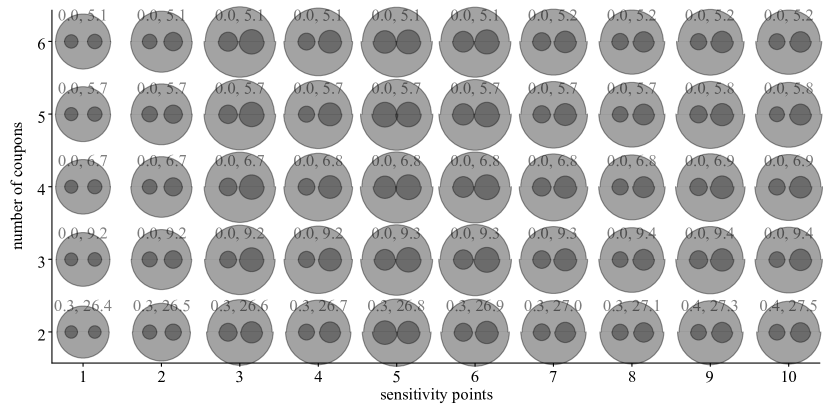
Figure 1: Relative performance of plain vanilla mean and VH estimators as point estimators for homophily topology, network of size 1000, uniform seed selection and preferential new respondent referral, with RDS processes of 2 to 6 coupons, and network topology sensitivity parameter at 10 different values. Every component of the plot consists of upper and lower sets of 3 half circles. Large half circles correspond to absolute difference in average MSE, left small half circles correspond to absolute difference in squared bias, and right small half circles correspond to absolute difference in variance. All differences are between the VH and plain mean estimator. Grey background color means positive sign, and white means negative sign. In this plot, there are no instances of a white background. Upper sets of half circles correspond to exact degree reporting, and lower sets correspond to random degree reporting. The pairs of numbers separated by commas mean the average number of times the RDS process had to restart, and the average number of waves needed to collect the sample with particular network topology and number of coupons, given other process features.

Strikingly, the plain mean outperforms the VH estimator across the board in both bias and variance. Some reasons for this can be gleaned from Figure 6. Better-connected nodes are in the center of the distribution of the underlying quantity, so the RDS process visits there often. The VH estimator suffers performance loss due to occasional low degrees of nodes in the center of the distribution, while the plain mean does not even use degree information!

Here 500 networks have been simulated for every sensitivity constant index, for computational reasons. This is small relative to the very large number of possible networks of size 1000 with specified topology. Therefore, figures such as Figure 1 should be construed as giving general trends in relative estimator performance.

3.4 Rich-get-richer networks

Figure 2 shows the relative performance of the plain mean and VH estimator for rich-get-richer networks of size 1000, and RDS processes with proportional to degree seed selection, and uniform participant referral. Note that the VH estimator outperforms the mean estimator across the board in MSE. The reason can be seen in Figure 6. Nodes with high degrees correspond to the tail of the distribution of the quantity of interest. Proportional to degree seed selection causes the process to visit the right tail more frequently, and the VH estimator does a better job discounting the corresponding observations because it weights them by inverse degree. The resulting bias reduction is sufficient to compensate for a worse variance.

Figure 2: Relative performance of plain vanilla mean and VH estimators as point estimators for rich-get-richer topology, network of size 1000, proportional to degree seed selection, uniform new respondent referral, with RDS processes of 2 to 6 coupons, and network topology sensitivity parameter at 10 different values. Graphical elements and numbers are as described in Figure 1.

Figure 2 demonstrates that the VH estimator has lower bias across the board, and the plain mean has better variance, especially in the case of stochastic degree reporting. However, for this case, bias reduction of the VH estimator is significant enough to give it an edge against the plain mean estimator. Here, random degree reporting helps the plain mean estimator gain ground against the VH estimator, since this smoothes out the low weights given by the VH estimator to the tail measurements.

The only setting when the VH estimator underperforms the plain mean for rich-get-richer networks is inverse preferential referral. In that setting, participants are referring people who are far away in the distribution, and thus the left tail of the distribution is visited more often (see Figure 6). Then the plain mean outperforms the VH estimator, as the VH estimator induces negative bias by up-weighting the left tail observations. The online resources described in Section 5 provide interactive visualizations of this phenomenon.

3.5 Number of coupons

We find that the number of coupons does not, in general, have a strong effect on the performance of the VH or plain mean estimator. Also, under the standard recruitment scheme, the RDS process does not need to be restarted to reach the necessary sample size, except in the 2-coupon case. The number of seeds has been set to agree with a survey of RDS studies (Malekinejad et al., 2008). To collect 300 observations, 2-coupon RDS processes yield unrealistically large numbers of waves. For 3-coupon RDS processes, 9 waves are obtained on average, which concurs with the average reported in (Malekinejad et al., 2008). RDS processes with 4, 5 and 6 coupons on average yield numbers of waves of 7, 6 and 5, respectively.

3.6 Sampling fraction

Our study considers two possible values for the sampling fraction. The sample size is 300, and network sizes are either 1000 or 3000, so the sampling fractions are 33% and 10%.

Figure 3: Relative performance of plain vanilla mean and VH estimators as point estimators for rich-get-richer topology, network of size 3000, proportional to degree seed selection, uniform new respondent referral, with RDS processes of 2 to 6 coupons, and network topology sensitivity parameter at 10 different values. Graphical elements and numbers are as described in Figure 1. The VH estimator dominates the plain mean in all setups here.

Generally, with the considered absolute sample size, sampling fraction has no effect on the patterns of estimator relative performance for every combination of simulation features. However, Figure 3 demonstrates that the VH estimator also has better variance than the plain mean in some instances, while Figure 2 corresponds to smaller network size and does not exhibit this observation. These findings suggest that for the sample sizes currently collected via RDS, sampling fraction is not a deciding factor for the choice of the estimation technique. This is encouraging, as in practice the sampling fraction is typically unknown.

3.7 Seed selection

In our simulations, we consider two seed selection mechanisms. The first is selecting the seeds at random from the set of network nodes, and the second is selecting the seeds with probability proportional to degree. Ideally, proportional to degree seed selection should favour the VH estimator, because it puts the process in ergodicity mode right away.

The idea behind exploring seed selection feature is to see how much of an improvement proportional to degree seed selection provides to the VH estimator in the settings when other assumptions it is based on are violated. We do not observe any cases when it does help the VH estimator outperform the plain mean. That is, at any combination of other simulation features, the picture of relative performance of the VH and plain mean estimators is the same regardless of seed selection mechanism.

Overall, we find that the possible improvement of the proportional to degree seed selection is overshadowed by other factors. We have even found some indication (under inverse homophily topology) that proportional to degree seed selection is detrimental for the VH estimator. Our online visualization resources can be used to explore this further (see Section 5).

3.8 Exact and stochastic degree reporting

In our simulations, reported values are drawn from a Poisson distribution with mean equal to true degree. With random degree reporting as defined in our study, there is little effect on the relative performance of the estimators. Under homophily, stochastic degree reporting further diminishes the performance of the VH estimator against the plain mean estimator for both sampling fractions considered (see Figures 1 and 4), and it has almost no effect for inverse homophily and rich-get-richer topologies. Still, it is possible that the current techniques of degree estimation may carry overdispersed error (Zheng et al., 2006; McCormick et al., 2010); the effect of uncertain degree reporting in real RDS studies remains largely unknown.

Figure 4: Relative performance of plain vanilla mean and VH estimators as point estimators for homophily topology, network of size 3000, proportional to degree seed selection, preferential new respondent referral, with RDS processes of 2 to 6 coupons, and network topology sensitivity parameter at 10 different values. Graphical elements and numbers are as described in Figure 1. Stochastic degree reporting harms the performance of the VH estimator in this case.

4 Overall performance comparison

The simulation results analyses presented so far have been carried out using sensitivity plots such as Figure 1. It is also useful to consider relative performance averaged over the network topologies sensitivity constants. We present the relevant findings in terms of summary tables containing average MSE for the plain mean and VH estimator for all simulation feature value combinations, constructed by network size and number of coupons.

Table 2: Average MSE for plain mean (numbers to the left from semicolons) and VH estimator (numbers to the right from semicolons; numbers to the right from commas correspond to random degree reporting) for different simulation configurations for networks of size 3000 and 3-coupon RDS. Cases when the VH estimator outperforms the plain mean are displayed in italic. There is a large discrepancy for rich-get-richer network topology and inverse preferential referral. Under homophily, the VH estimator is dominated by the plain mean under all settings.

	referral function
Network, seed	unif	pref	inv pref
homo, unif s	14.46; 46.51, 48.57	28.73; 71.48, 73.54	3.08; 25.84, 29.28
homo, pr to deg s	8.83; 21.52, 22.03	16.84; 30.22, 30.52	2.13; 15.98, 18.4
inv homo, unif s	1.05; 0.32, 0.32	0.99; 0.28, 0.28	2.4; 3.32, 3.32
inv h, pr to deg s	1.07; 0.33, 0.33	1.01; 0.3, 0.3	2.45; 3.84, 3.84
r-g-r, unif seed	4.08; 0.24, 0.25	13.11; 8.62, 8.61	2.35; 43.75, 43.91
r-g-r, pr to deg s	4.24; 0.24, 0.24	18.44; 12.11, 12.1	2.35; 43.6, 43.77

Table 2 summarizes the relative performance of the plain mean and VH estimator for networks of size 3000, and 3-coupon RDS. Under homophily, the VH estimator is dominated by the mean in all settings. For rich-get-richer networks with inverse preferential referral, the plain mean does much better than VH. Under all other scenarios, VH outperforms the plain mean. In these simulations, random degree reporting has little effect on the performance of the VH estimator except for a small detrimental effect in homophily networks.

Table 3: Average MSE for plain mean (numbers to the left from semicolons) and VH estimator (numbers to the right from semicolons; numbers to the right from commas correspond to random degree reporting) for different simulation configurations for networks of size 1000 and 6-coupon RDS. Cases when the VH estimator outperforms the plain mean are displayed in italic. Overall, there is little change in relative performance of the two considered estimators from what is observed in Table 2.

	referral function
Network, seed	unif	pref	inv pref
homo, unif s	12.88; 40.08, 43.52	18.55; 49.08, 52.55	6.11; 29.02, 33.12
homo, pr to deg s	8.71; 20.77, 21.98	12.79; 25.33, 26.3	4.12; 16.55, 18.99
inv homo, unif s	2.72; 1.53, 1.51	2.5; 1.33, 1.31	4.34; 8.75, 8.76
inv h, pr to deg s	2.98; 1.63, 1.61	2.77; 1.4, 1.38	4.58; 9.87, 9.9
r-g-r, unif seed	3.2; 0.31, 0.33	9.6; 5.01, 4.99	4.24; 24.29, 24.53
r-g-r, pr to deg s	3.29; 0.3, 0.31	13.59; 7.31, 7.28	4.28; 23.83, 24.07

Table 3 contains summary of relative performance of the VH and plain mean estimator for networks of size 1000 and 6-coupon RDS. Similarly to 3-coupon RDS, the VH estimator underperforms on homophily networks under all scenarios.

5 Interpretation and visualization

Our simulation methods allow us easily to explore the bias-variance trade-off for the VH and plain mean estimator for a particular network topology sensitivity constant, and a given combination of other RDS features. For example, Figure 5 shows the squared bias, variance and MSE histograms of the plain mean and VH estimators for simulated RDS processes on networks with size 3000, network topology sensitivity constant 5, proportional to degree seed selection and uniform participant referral.

Figure 5: Estimated densities of squared biases, variances and MSE of plain vanilla mean and VH estimators for RDS, homophily network of size 3000, topology sensitivity constant 5, 3 coupon structure, proportional to degree seed selection, uniform referral and exact degree reporting. Straight lines represent density means. The mean outperforms the VH estimator in all aspects, with a much lower variance, and similar squared bias.

Such figures help give insight into what performance components of an estimator suffer a larger loss relative to another on a given network topology and RDS features. Figure 6 displays the relationship between quantity of interest and degrees of bearing vertices for different network topologies.

Figure 6: Histogram of RDS quantity of interest and scatterplot of normalized degrees, for inverse homophily (left), homophily (center) and rich-get-richer (right) networks.

To develop relevant intuition, let us consider an example of how Figure 6 is used. A notable finding from Table 3 is that the VH estimator outperforms the mean when the network is explored with uniform or preferential referral function, on inverse homophily and rich-get-richer topologies. With uniform and preferential referral functions, nodes with high degrees get visited more often, so more tail measurements get into the RDS sample (see Figure 6). The VH estimator weights observations by inverse degree, thus discounting the tail measurements. The plain mean, on the other hand, gives equal weights to all observations in the sample. This makes the plain mean estimator have large bias and larger variance than the VH estimator.

The VH estimator shines if the underlying network topology is such that vertices bearing tail measurements have high degrees. This is because it gives high weights to measurements from the middle of distribution, thus having both low bias and variance. This is well illustrated with Figure 7, which shows inverse homophily. Under preferential and uniform referral functions, high degree vertices are visited more often and thus tail measurements get into the RDS sample more frequently (see Figure 6). This hinders the performance of the plain mean and gives an edge to the VH estimator.

Analogously, for homophily networks, the plain mean outperforms VH (see Figure 5). In this setting, the mean wins by weighting all measurements equally as the RDS process stays near the center of distribution most of the time, while the VH estimator down-weights them.

Figure 7: Estimated densities of squared biases, variances and MSE of plain vanilla mean and VH estimators for RDS, inverse homophily network of size 3000, topology sensitivity constant 5, 3 coupon structure, proportional to degree seed selection, uniform referral and exact degree reporting. Straight lines represent density means. The VH estimator outperforms the plain mean in all aspects, with a lower variance and squared bias.

Weighting observations by inverse degree puts the VH estimator in its most unfavorable situation when operating under inverse preferential referral function. When this function governs the RDS process, respondents try to refer next participants far from them in the distribution of the quantity of interest. The most vivid example is rich-get-richer networks with inverse preferential referral, when the mean outperforms the VH estimator by more than tenfold in terms of MSE (for example, see the bottom right of Table 2). This happens because the left tail is frequently visited due to inverse preferential referral function (see Figure 6), and the VH estimator overweights these observations because they have low degrees. This induces large negative bias, thus putting the VH estimator far behind.

We have made available online two supplementary visualizations: an interactive visualization of the plain mean and VH estimator tradeoffs for all settings described in this paper, with additional results presented for smaller scale simulations, and an interactive visualization of RDS processes with varying network topologies, as a function of the quantity surveyed; see http://incontemplation.com/go/rdsdynamic1 and http://incontemplation.com/go/rdsdynamic2.

6 Discussion

In this work, we have explored several key aspects of RDS for various network topologies dependent on the quantity surveyed. This makes it possible to compare estimation performance of various simulation features. We attempt to quantify the extent to which degree information is needed for adequate estimation, and identify the driving features that make one estimator underperform and another dominate in various settings.

A limitation of our work is that it focuses on a univariate quantity of interest, with a small number of particular methods of generating network topology dependent on the quantity of interest. It would be interesting to develop alternative methods with different network topologies but similar associations of degree and quantity of interest.

Our findings suggest that using inverse-to-estimated-degree weightings for RDS estimation is questionable under many circumstances. In other simulations we have also explored compromise estimators, with the VH weights raised to a fractional power. These estimators smoothly interpolate between the plain mean and the VH estimator, but there is much scope for developing and selecting between various compromise estimators. The results show that special care should be given to the role of homophily in RDS, and the interplay between the network structure, recruitment preference patterns, and the quantity of interest.

7 Acknowledgements

We thank Edoardo Airoldi, Victor DeGruttola, Richard Garfein, and Susan Little for helpful comments. Joseph Blitzstein acknowledges NIH P01 AI074621 for partial support, and Sergiy Nesterko acknowledges the Natural Sciences and Engineering Research Council of Canada via Postgraduate Scholarship 90350447 for partial support.

References

- Abramovitz et al. [2009] D. Abramovitz, E. M Volz, S. A Strathdee, T. L Patterson, A. Vera, and S. D.W Frost. Using respondent driven sampling in a hidden population at risk of HIV infection: Who do HIV-positive recruiters recruit? Sexually transmitted diseases, 36(12):750, 2009.
- Frost et al. [2006] S. D.W Frost, K. C Brouwer, M. A Firestone Cruz, R. Ramos, M. E Ramos, R. M Lozada, C. Magis-Rodriguez, and S. A Strathdee. Respondent-driven sampling of injection drug users in two US–Mexico border cities: recruitment dynamics and impact on estimates of HIV and syphilis prevalence. Journal of Urban Health, 83:83–97, 2006.
- Gile and Handcock [2010] Krista J. Gile and Mark S. Handcock. Respondent-driven sampling: An assessment of current methodology. Sociological Methodology, 40, 2010.
- Goel and Salganik [2010] Sharad Goel and Matthew J. Salganik. Assessing respondent-driven sampling. PNAS, 107 (15):6743––6747, 2010.
- He et al. [2008] Qun He, Ye Wang, Yan Li, Yurun Zhang, Peng Lin, Fang Yang, Xiaobing Fu, Jie Li, H. Fisher Raymond, Li Ling, and Willi McFarland. Accessing men who have sex with men through Long-Chain referral recruitment, Guangzhou, China. AIDS and Behavior, 12(S1):93–96, April 2008. doi: 10.1007/s10461-008-9388-y.
- Heckathorn [1997] Douglas D. Heckathorn. Respondent-driven sampling: A new approach to the study of hidden populations. Social Problems, 44:174–199, 1997.
- Heckathorn [2002] Douglas D. Heckathorn. Respondent-driven sampling ii: Deriving valid population estimates from chain-referral samples of hidden populations. Social Problems, 49:11–34, 2002.
- Lansky et al. [2007] A. Lansky, A. S Abdul-Quader, M. Cribbin, T. Hall, T. J Finlayson, R. S Garfein, L. S Lin, and P. S Sullivan. Developing an HIV behavioral surveillance system for injecting drug users: the national HIV behavioral surveillance system. Public Health Reports, 122(Suppl 1):48, 2007.
- Lu et al. [2011] X. Lu, L. Bengtsson, T. Britton, M. Camitz, B. J Kim, A. Thorson, and F. Liljeros. The sensitivity of respondent-driven sampling method. Journal of the Royal Statistical Society A, 2011.
- Magnani et al. [2005] R. Magnani, K. Sabin, T. Saidel, and D. Heckathorn. Review of sampling hard-to-reach and hidden populations for HIV surveillance. AIDS, 19:S67, 2005.
- Malekinejad et al. [2008] Mohsen Malekinejad, Lisa Grazina Johnston, Carl Kendall, Ligia Regina Franco Sansigolo Kerr, Marina Raven Rifkin, and George W. Rutherford. Using Respondent-Driven sampling methodology for HIV biological and behavioral surveillance in international settings: A systematic review. AIDS and Behavior, 12(S1):105–130, June 2008. doi: 10.1007/s10461-008-9421-1.
- McCormick et al. [2010] T. H McCormick, M. J Salganik, and T. Zheng. How many people do you know?: Efficiently estimating personal network size. Journal of the American Statistical Association, 105(489):59–70, 2010.
- Salganik [2006] M. J Salganik. Variance estimation, design effects, and sample size calculations for respondent-driven sampling. Journal of Urban Health, 83:98–112, 2006.
- Salganik and Heckathorn [2004] Matthew J. Salganik and Douglas D. Heckathorn. Sampling and estimation in hidden populations using respondent-driven sampling. Sociological Methodology, 34:193–240, 2004.
- Tomas and Gile [2010] A. Amber Tomas and Krista J. Gile. The effect of differential recruitment, non-response and non-recruitment on estimators for Respondent-Driven sampling. arXiv:1012.4122, 2010.
- Volz and Heckathorn [2008] Erik Volz and Douglas D. Heckathorn. Probability based estimation theory for respondent driven sampling. Journal of Official Statistics, 24 (1):79–97, 2008.
- Zheng et al. [2006] T. Zheng, M. J Salganik, and A. Gelman. How many people do you know in prison? Journal of the American Statistical Association, 101(474):409–423, 2006.