UPR-1243-T

MPP-2012-126

Anomaly Cancellation And
Abelian Gauge Symmetries In F-theory

Mirjam Cvetič^1,2, Thomas W. Grimm³ and Denis Klevers¹

$\,{}^{1}$ Department of Physics and Astronomy,

University of Pennsylvania, Philadelphia, PA 19104-6396, USA

$\,{}^{2}$ Center for Applied Mathematics and Theoretical Physics,

University of Maribor, Maribor, Slovenia

$\,{}^{3}$ Max-Planck-Institut für Physik,

Föhringer Ring 6, 80805 Munich, Germany

cvetic at cvetic.hep.upenn.edu, grimm at mpp.mpg.de, klevers at sas.upenn.edu

ABSTRACT

We study 4D F-theory compactifications on singular Calabi-Yau fourfolds with fluxes. The resulting $\mathcal{N}=1$ effective theories can admit non-Abelian and $U(1)$ gauge groups as well as charged chiral matter. In these setups we analyze anomaly cancellation and the generalized Green-Schwarz mechanism. This requires the study of 3D $\mathcal{N}=2$ theories obtained by a circle compactification and their M-theory duals. Reducing M-theory on resolved Calabi-Yau fourfolds corresponds to considering the effective theory on the 3D Coulomb branch in which certain massive states are integrated out. Both 4D gaugings and 3D one-loop corrections of these massive states induce Chern-Simons terms. All 4D anomalies are captured by the one-loop terms. The ones corresponding to the mixed gauge-gravitational anomalies depend on the Kaluza-Klein vector and are induced by integrating out Kaluza-Klein modes of the $U(1)$ charged matter. In M-theory all Chern-Simons terms classically arise from $G_{4}$-flux. We find that F-theory fluxes implement automatically the 4D Green-Schwarz mechanism if non-trivial geometric relations for the resolved Calabi-Yau fourfold are satisfied. We confirm these relations in various explicit examples and elucidate the general construction of $U(1)$ symmetries in F-theory. We also compare anomaly cancellation in F-theory with its analog in Type IIB orientifold setups.

October, 2012

1 Introduction and Summary

Local symmetries are the guiding principle for formulating field theories as well as the theory of gravity. While manifest in the classical theory these symmetries can, however, be broken at the quantum level and lead to inconsistencies by the violation of essential current conservation laws on the quantum level. Such inconsistencies manifest themselves already at one-loop level and are known as anomalies [1]. In particular, four-dimensional quantum field theories can admit anomalies which signal the breaking of the gauge symmetry transformations acting on chiral fermions. The cancellation of these anomalies is thus crucial to determine consistent theories and imposes constraints on the spectrum and couplings of the theory. Anomalous transformations of the chiral fermions either cancel among each other or require the implementation of a generalized Green-Schwarz mechanism [2, 3]. In the latter case the one-loop anomalies are canceled by a tree-level diagram involving a $U(1)$ gauged axion-like scalar. In this work we study the manifestation of the anomaly cancellation mechanisms in four-dimensional F-theory compactifications.

To extract four-dimensional observed physics from string theory one is aiming to find a compactification scenario that describes a very broad class of consistent string vacua and naturally incorporates the ingredients of the Standard Model of particle physics and its extensions. One promising scheme is to consider F-theory compactifications with space-time filling seven-branes supporting non-Abelian gauge groups. F-theory geometrizes the complexified coupling constant of Type IIB string theory as the complex structure modulus of an additional two-torus. Much of the in general non-perturbative physics of seven-branes is encoded in the singular geometry of a torus-fibered compact manifold. Requiring $\mathcal{N}=1$ supersymmetry in the four-dimensional effective theory enforces this space to be an elliptically fibered Calabi-Yau fourfold $X_{4}$. The complex three-dimensional base $B_{3}$ of $X_{4}$ is the physical compactification space of Type IIB string theory. The singularities of this fourfold along co-dimension one loci in the base signal the presence of non-Abelian gauge groups, while additional sections of the elliptic fibration signal extra $U(1)$ gauge group factors [4, 5].

A non-trivial four-dimensional chiral spectrum is only induced if the seven-branes also support gauge fluxes on their internal world volume. The interplay of geometry, fluxes and the low-energy effective action of the four-dimensional gauge theory is crucial in the study of anomaly cancellation. However, the fact that F-theory does not posses a low-energy effective action in twelve dimensions prevents one from deriving the four-dimensional low-energy effective theory directly. To nevertheless study F-theory effective physics one has to use the M-theory dual description in one dimension lower. In fact, M-theory on the same Calabi-Yau fourfold $X_{4}$ is dual to F-theory on $X_{4}\times S^{1}$. The new modulus, the radius of $S^{1}$, is in this identification related to the inverse volume of the torus fiber in M-theory. In this duality, the familiar F-theory limit of a shrinking volume of the torus-fiber maps to the decompactification limit of the $S^{1}$ in which one grows a large extra dimension and recovers four dimensional F-theory physics. All F-theory objects can then be followed through this three-dimensional duality and can be studied directly in the dual M-theory. In this work we will mainly be interested in questions about the low energy physics of F-theory, most prominently anomalies, and it will be one of our results to reformulate and answer these questions in M-theory.

At low energies the theory of interest is an effective three-dimensional (3D) $\mathcal{N}=2$ gauge theory with a number of chiral multiplets coupled to supergravity. An important property of the 3D $\mathcal{N}=2$ gauge theories is that they admit, in contrast to a $\mathcal{N}=1$ gauge theory in four dimensions (4D), a Coulomb branch where the non-Abelian gauge group $G$ breaks to its maximal torus, $G\rightarrow U(1)^{r}$, with massless 3D gauge fields $A^{\Lambda}$, $\Lambda=1,\ldots,r=\text{rank}(G)$. In this work we will mainly analyze the theory on this 3D Coulomb branch and understand corrections to the effective action both from the F-theory perspective and from the M-theory perspective.

There is one essential difference between the two descriptions of the 3D theory, that is crucial for this discussion. By reducing F-theory from 4D to 3D we can describe the 3D $\mathcal{N}=2$ gauge theory also away from the Coulomb branch. The Coulomb branch is understood purely field theoretically by giving a vacuum expectation value (vev) to the scalars $\zeta^{\Lambda}$ along the Cartan generators of $G$ in the 3D vector multiples coming from the direction of the 4D vector along the $S^{1}$. Fields become massive due to this vev and at low energies have to be integrated out quantum mechanically correcting the effective theory on the Coulomb branch. In contrast, although M-theory as a fundamental theory should also describe the full 3D $\mathcal{N}=2$ gauge theory, it is only explicitly known how to describe the 3D Coulomb branch. The description is given by M-theory on the smooth $\hat{X}_{4}$ fourfold with all singularities in $X_{4}$ resolved inducing shrinkable rational curves, i.e. two-spheres $\mathbb{P}^{1}$, in the geometry. Geometrically, the resolution process corresponds to giving a vev in the field theory perspective with $\zeta^{\Lambda}$ being related to the volume of these shrinkable $\mathbb{P}^{1}$’s. Furthermore, at large volume of $\hat{X}_{4}$ it is consistent to consider the long wavelength approximation of eleven-dimensional supergravity and dimensionally reduce it on $\hat{X}_{4}$ to 3D. In this description certain microscopic M-theory degrees of freedom corresponding to certain wrapped M2-branes are massive. However, these states have already been integrated out consistently in the eleven-dimensional supergravity, which follows from the validity and consistency of the supergravity approximation at low energies. The corrections to the 3D low-energy theory on the Coulomb branch are thus visible as classical effects in the dimensional reduction on $\hat{X}_{4}$. Morally speaking, the information about the massless microscopic states on $X_{4}$ has been traded for the new shrinkable $\mathbb{P}^{1}$’s on $\hat{X}_{4}$, that have not been present on $X_{4}$. These corrections are the same as those that arise quantum mechanically in F-theory and it will be one key observation of this paper to map these corrections in the M-/F-theory duality in 3D.

The geometrically massive modes that have to be integrated out on the 3D Coulomb branch and are relevant for our discussion of anomalies are from an F- and M-theory point of view

• massive 3D W-bosons in F-theory from the breaking $G\rightarrow U(1)^{r}$, or massive M2-branes on shrinking $\mathbb{P}^{1}$’s in $\hat{X}_{4}\rightarrow X_{4}$ over co-dimension one in $B_{3}$ in M-theory.

• charged 3D fermions massive on the 3D Coulomb branch in F-theory, or massive M2-branes on $\mathbb{P}^{1}$’s fibered over co-dimension two in $B_{3}$, i.e. curves from intersections of seven-branes in F-theory later denoted as matter curves, in M-theory.

• massive Kaluza-Klein states of 4D charged fermions in the reduction of F-theory from 4D to 3D, or M2-branes wrapping a shrinking $\mathbb{P}^{1}$ over a matter curve once and multiply the elliptic fiber of $\hat{X}_{4}$.

The 3D couplings that are corrected by integrating out these massive states and that will be of most use for our discussion of 4D anomalies in F-theory are the 3D Chern-Simons (CS) terms for the Abelian vector fields $A^{\Lambda}$ on the 3D Coulomb branch,

$$S^{(3)}_{CS}=-\frac{1}{2}\int\Theta_{\Lambda\Gamma}A^{\Lambda}\wedge F^{\Gamma}\,.$$ (1)

Again, the crucial point is that from the F-theory perspective these CS-terms are purely quantum mechanically and generated only at one-loop of massive fermions charged under the vectors $A^{\Lambda}$. In contrast on the M-theory side they are generated classically by $G_{4}$-flux on $\hat{X}_{4}$. Thus, the CS-terms still carry the signature of the states that have been integrated out in F-theory but are efficiently calculated in M-theory. More precisely we will use in this work as a tool to derive the chiral index $\chi(\mathbf{R})$ of 4D charged matter in a representation $\mathbf{R}$ the observation of [6] that certain $G_{4}$-fluxes induce particular classical M-theory CS-terms which are induced in F-theory by one-loop diagrams of the 3D massive charged fermions from the 4D chiral matter multiplets reduced on $S^{1}$. The identification of classical M- and one-loop F-theory CS-terms $\Theta_{\Lambda\Sigma}^{M}$ respectively $\Theta_{\Lambda\Sigma}^{F}$ we will employ takes the form

$$\frac{1}{2}\Theta_{\Lambda\Sigma}^{M}=\frac{1}{4}\int_{\hat{X}_{4}}G_{4}\wedge\omega_{\Lambda}\wedge\omega_{\Sigma}\equiv-\frac{1}{2}\sum_{\mathbf{R}}\chi(\mathbf{R})\sum_{q\in\mathbf{R}}q_{\Lambda}q_{\Sigma}\ \text{sign}(q\cdot\zeta)=-\Theta^{F}_{\Lambda\Sigma}\,,$$ (2)

where $\omega_{\Lambda}$, $\omega_{\Sigma}$ denote $(1,1)$-forms on $\hat{X}_{4}$ generated by resolving the singularities in $X_{4}$ and the sum is taken over all 4D matter representations $\mathbf{R}$ with Dynkin labels $q$. The sign-function is applied to the scalar product of the charges and the Coulomb branch parameters, $q\cdot\zeta=q_{\Lambda}\,\zeta^{\Lambda}$. In general, M-theory $G_{4}$-flux on the fully resolved Calabi-Yau $\hat{X}_{4}$ that is consistent with the F-theory limit is the description of seven-brane gauge flux in F-theory. Thus, as is known that gauge fluxes on seven-branes induce chirality of 4D matter in Type IIB $G_{4}$-flux induces chirality in F-theory. The relation of such fluxes to the 4D matter spectrum has been recently studied intensively [7, 8, 9, 10, 11, 12, 13, 6, 14, 15].

Besides using the CS-terms in 3D as tools for determining 4D chirality we will discover the intricate relations between different 3D CS-terms that are implied by 4D anomaly cancellation. Let us summarize our findings where we distinguish F-theory compactifications without Abelian gauge symmetries and those with Abelian gauge factors. In the first case it is required that the non-Abelian gauge anomaly vanishes which puts one constraint on the spectrum for each gauge group factor $G_{(I)}$ in $G$ whereas in the second case anomaly cancellation is more involved due to mixed anomalies. The cancellation of these anomalies may require a Green-Schwarz (GS) mechanism in F-theory. Then fluxes on space-time filling seven-brane have to both induce a non-trivial chiral spectrum and corresponding gaugings of the axions for a working GS-mechanism. Anomaly cancellation is then tightly linked with tadpole cancellation that imposes constraints on the brane configuration and allowed fluxes. For setups at weak string coupling this link has been discussed and reviewed, for example, in [16, 17, 18, 19, 20, 21].

In contrast to the weakly coupled Type IIB theory, where brane fluxes are constrained by tadpole conditions, for $G_{4}$ fluxes lifting from M-theory to F-theory it is expected that all anomalies are canceled and the Green-Schwarz mechanism is implemented automatically. This can be anticipated since in M-theory no additional consistency conditions on $G_{4}$, apart from the for anomaly cancellation irrelevant M2-brane tadpole matching, have to be imposed. In particular the seven-brane tadpole is canceled geometrically in F-theory by considering a compact Calabi-Yau fourfold $X_{4}$ and 5-brane tadpoles are canceled by considering closed fluxes $dG_{4}=0$ signalling the absence of a net M5-brane charge. Therefore, by consistency of the underlying M-theory compactification also the low-energy effective action should be consistent.

From anomaly cancellation in combination with F-/M-theory duality in 3D we discover the following constraints for and links to 3D CS-terms:

• Without $U(1)$-factors in 4D, the CS-terms for the vectors $A^{\Lambda}$ encoding chiralities have to obey non-trivial relations such that the cubic non-Abelian anomalies are canceled.

• With $U(1)$-factors in 4D, the CS-terms for the 4D chiral indices have to be related to the CS-terms determining the gaugings of the 4D axions so that all mixed anomalies are canceled.

• We show the cancellation of 4D mixed Abelian-gravitational anomalies in 3D using F-/M-theory duality. We discover that the 4D mixed Abelian-gravitational anomaly is the coefficient $\Theta^{\text{loop}}_{0m}$ of the 3D Chern-Simons term $A^{0}\wedge F^{m}$ for the Kaluza-Klein vector $A^{0}$ and the corresponding 3D $U(1)$ vector field $A^{m}$,

  $$\Theta^{\text{loop}}_{0m}=-\frac{1}{12}\sum_{\underline{q}}n(\underline{q})q_{m}\,,$$ (3)

  where the sum is taken over all $U(1)$-charges $\underline{q}$ under the 4D $U(1)$-vectors $A^{m}$ and $n(\underline{q})$ is the number of fermions with a given charge $\underline{q}$. We obtain this result since $\Theta_{0m}$ is one-loop induced in F-theory with the full Kaluza-Klein tower of 4D charged fermions in the loop. F-/M-theory duality implies that this expression is related to the classical flux-integral of $G_{4}$ in M-theory, which is precisely the tree-level contribution to the anomaly from the GS-mechanism,

  $$\Theta^{\text{loop}}_{0m}\equiv-\frac{1}{2}\Theta_{0m}=\frac{1}{4}K^{\alpha}\Theta_{\alpha m}\,.$$ (4)

  Here $K^{\alpha}$ is a vector determining a direction in the space of 4D axions and $\Theta_{m\alpha}$ is the $G_{4}$-flux induced gauging of the $\alpha$th axion under $A^{m}$.

In addition, we discuss in general terms the construction of $U(1)$ symmetries in F-theory on fourfolds by considering a non-trivial Mordell-Weil group of rational sections of $\hat{X}_{4}$. This construction has been applied successfully on elliptically fibered threefolds in [5, 22, 23, 24] to study non-simply laced gauge groups and $U(1)$’s as well as Abelian anomalies in six-dimensional F-theory. The discussion we provide in this note is a first step to being able to construct also four-dimensional F-theory compactifications with more than one $U(1)$ and a matter sector with more general $U(1)$-charges extending the analysis of [25].

Furthermore, for consistent $G_{4}$-fluxes in the F-theory limit, we discover geometric relations that need to be satisfied in any resolved elliptically fibered fourfold $\hat{X}_{4}$,

$$\frac{1}{3}\sum_{S_{\mathbf{R}}}\sum_{c\,\subset S_{\mathbf{R}}}(S_{\mathbf{R}}\cdot[G_{4}])(c\cdot D_{\Lambda})(c\cdot D_{\Sigma})(c\cdot D_{\Gamma}) = \frac{1}{2}[G_{4}]\cdot D_{(\Gamma}\cdot\pi_{*}(D_{\Lambda}\cdot D_{\Sigma)})\ ,$$ (5)

$$\frac{1}{3}\sum_{S_{\mathbf{R}}}\sum_{c\,\subset S_{\mathbf{R}}}(S_{\mathbf{R}}\cdot[G_{4}])(c\cdot D_{\Lambda}) = [G_{4}]\cdot[c_{1}(B_{3})]\cdot D_{\Lambda}\,.$$ (6)

Here $G_{4}$ is the $G_{4}$-flux in M-theory and $S_{\mathbf{R}}$ is a four-cycle denoted the matter surfaces obtained by fibering the shrinking $\mathbb{P}^{1}$’s in $\hat{X}_{4}$ that are the weights of a representation $\mathbf{R}$ of $G$ over matter curves. The divisors $D_{\Lambda}$, $D_{\Sigma}$ and $D_{\Gamma}$ are the exceptional divisors obtained by fibering the shrinkable curves $\mathbb{P}^{1}$ over co-dimension one loci in the base $B_{3}$, i.e. the seven-brane divisors in $B_{3}$. The curves $c$ are any shrinkable holomorphic curve in the fiber $S_{\mathbf{R}}$. The map $\pi_{*}$ is induced by the projection to the base $\pi\,:\,\hat{X}_{4}\rightarrow B_{3}$ of the elliptic fibration of $\hat{X}_{4}$ and $c_{1}(B_{3})$ denotes its first Chern-class. These geometric relations are indeed valid for concrete resolutions as we show for several examples with non-Abelian gauge groups.

We note that the geometric relations (5) and the corresponding statements about anomaly cancellation should even apply in a broader context than considered in this paper. In particular one expects that (5) is valid for more general $G_{4}$-flux that is not necessarily given by a sum of products of $(1,1)$-forms, i.e. $G_{4}$-flux that is not vertical. A phenomenologically interesting example of these fluxes is the F-theory analog of hypercharge flux $F_{Y}$ considered in [26, 27, 28] in the context of anomalies. In order to understand anomaly cancellation also in these cases, it is crucial to note that the right hand side of (5) is in general only non-trivial for vertical $G_{4}$-flux and vanishes otherwise. Constraints on the spectrum then arise from the vanishing of the left-hand side of this equality. A better understanding of the global geometry of $\hat{X}_{4}$ and the matter surfaces $S_{\mathbf{R}}$ might reveal that these constrains are also automatic fulfilled for concrete resolved Calabi-Yau fourfolds with no further restriction on the $G_{4}$-flux. It would be interesting to investigate this further.

Finally, we compare our analysis of anomaly cancellation in F-theory to anomaly cancellation in Type IIB Calabi-Yau orientifold compactifications with O7-planes and intersecting D7-branes [17, 18, 19, 20]. We show that in general the Type IIB anomaly cancellation reduces to the F-theory anomaly cancellation when projecting to the sector of geometrically massless $U(1)$’s in Type IIB. This demonstrates on the levels of anomalies that the geometrically massless $U(1)$’s correspond directly to the $U(1)$’s engineered in F-theory, whereas the geometrically massive $U(1)$’s in Type IIB are captured by the residual discriminant of the elliptic fibration in F-theory, cf. [29] for a more general discussion of geometrically massive $U(1)$’s.

The paper is organized as follows. In section 2 we recall some basic facts about anomaly cancellation in 4D and introduce the Green-Schwarz mechanism. In order to determine the Green-Schwarz counter terms in F-theory we discuss the geometric structure of resolved Calabi-Yau fourfolds used in the duality of M-theory to F-theory in section 3. It will be crucial to allow for $U(1)$ gauge group factors and their geometric F-theory manifestation in our analysis. In section 4 we turn to the analysis of one-loop Chern-Simons terms in the 3D effective theory. We recall how they encode the 4D chiral index for the matter spectrum and show that they can also capture 4D mixed Abelian/gravitational anomalies. Anomaly cancellation in F-theory is discussed in section 5 were we also derive the geometric conditions (5). We contrast the F-theory analysis with the description of anomaly cancellation in weakly coupled Type IIB setups with D7-branes and O7-planes in section 6. Explicit examples of resolved Calabi-Yau fourfolds are introduced in section 7. Our work has two appendices supplementing additional information about 4D anomalies and $SU(5)$ representations.

2 Four-Dimensional Anomaly Cancellation

In this section we present the basic techniques for characterizing anomalies of gauge symmetries and their cancellation via the generalized Green-Schwarz mechanism in a four dimensions. More details can be found in appendix A and the reviews [1].

We will consider a 4D $\mathcal{N}=1$ supersymmetric effective theory with a vector multiplet transforming in the adjoint of a general non-Abelian gauge group,

$$G=G_{(1)}\times\cdots\times G_{(n_{G})}\times U(1)_{1}\times\cdots\times U(1)_{n_{U(1)}}\,.$$ (7)

Here the group factors $G_{(I)}$ denote $n_{G}$ arbitrary simple Lie-groups and we allow for a number $n_{U(1)}$ of $U(1)_{m}$-factors. In the following we will use indices

$$I,J=1,\ldots,n_{G}\ ,\qquad\quad m,n=1,\ldots,n_{U(1)}\ ,$$ (8)

to label non-Abelian and Abelian group factors. We consider matter in chiral multiplets that transform in representations denoted

$$\mathbf{R}=(\mathbf{r}^{1},\ldots,\mathbf{r}^{n_{G}})_{\underline{q}}\,$$ (9)

of $G$. Here $\mathbf{r}^{I}$ denote the representations of the non-Abelian factors of $G_{(I)}$ and $\underline{q}=(q_{1},\ldots,q_{n_{U(1)}})$ denotes the corresponding $U(1)$-charges arranged as a column vector. Furthermore, since we are considering a theory with $\mathcal{N}=1$ supersymmetry we have one gravity multiplet containing a single gravitino.

In general an anomaly of a symmetry denotes the effect that a symmetry of the classical theory is not promoted to a symmetry of the quantum theory. An anomaly of a local symmetry, i.e. a gauge symmetry, spoils the consistency of the quantum theory due to the quantum mechanical violation of current conservation laws. Thus in a consistent quantum theory anomalies of gauge symmetries have to be absent. The breakdown of a gauge symmetry is encoded in a gauge invariant and regulator independent way in the anomaly polynomial. In four dimensions this polynomial is a cubic polynomial in the gauge field strength of the gauge group $G$ and the 4D Riemann tensor. Thus, it is a formal six-form denoted by $I_{6}$. The polynomial $I_{6}$ is the sum of the anomaly polynomials for all fields contributing to the anomaly. These are massless Weyl-fermions, gravitinos and self-dual tensors and their corresponding anomaly polynomials have been worked out in every space-time dimension in the seminal work of [30]. The theory is anomaly free if the full anomaly polynomial vanishes identically, i.e. if all coefficients of the various monomials in the field strength and the Riemann tensor are zero. As we will discuss next, the full anomaly polynomial consistent of $I_{6}$ from the quantum anomalies in the matter sector and another contribution from a tree-level effect, the Green- Schwarz mechanism.

In four dimensions, the possible anomalies are gauge and mixed anomalies only, since pure gravitational anomalies are absent by symmetry. For the fields in the standard $\mathcal{N}=1$ supergravity theory described above the anomaly polynomial reads

$$I_{6}=\sum_{\mathbf{R}}n(\mathbf{R})I_{1/2}(\mathbf{R})\,,$$ (10)

where $I_{1/2}(\mathbf{R})$ denotes the anomaly polynomial (157) of a left-chiral Weyl fermion that occurs with multiplicity $n(\mathbf{R})$ in the 4D spectrum.

In general, the anomaly polynomial (10) of the matter sector does not need to vanish identically if it is a sum of factorizable contributions. In this case, the residual anomalies can be canceled by a certain tree-level mechanism known as the Green-Schwarz mechanism [2]. We consider the higher derivative effective action, referred to as the Green-Schwarz counter terms,

$$S^{(4)}_{\rm GS}=-\frac{1}{8}\int\frac{2}{\lambda_{I}}b_{I}^{\alpha}\rho_{\alpha}\ \text{tr}_{\textbf{f}}\,(F^{I}\wedge F^{I})+2b_{mn}^{\alpha}\rho_{\alpha}\ F^{m}\wedge F^{n}-\frac{1}{2}a^{\alpha}\rho_{\alpha}\ \text{tr}(R\wedge R)\ .$$ (11)

Here $F^{I}$ and $F^{m}$ denote the field strengths in the adjoint of $G_{(I)}$ respectively of the $m$-th $U(1)$ and $\text{tr}_{\mathbf{f}}$ denote the traces in the corresponding fundamental representations. Furthermore, we have used $\lambda_{I}=2c_{G_{(I)}}/V(\mathbf{adj})=\frac{2}{\langle\alpha_{0},\alpha_{0}\rangle}$ with $c_{G_{(I)}}$ the dual Coxeter number of $G_{(I)}$ and $V(\mathbf{adj})$ defined in (162), whereas $\langle\alpha_{0},\alpha_{0}\rangle$ denotes the length squared of the root of maximal length $\alpha_{0}$. The real scalar fields $\rho_{\alpha}$ are axions that are gauged by the Abelian vectors $A^{m}$ of $G$ as

$$\mathcal{D}\rho_{\alpha}=d\rho_{\alpha}+\Theta_{\alpha m}\,A^{m}\,.$$ (12)

The combinations of axions $\rho_{\alpha}$ in the various terms in (11) are determined by parameters $b^{\alpha}_{I}$, $b^{\alpha}_{mn}$ and $a^{\alpha}$, which can be determined by the underlying microscopic theory together with the matrix $\Theta_{\alpha m}$ in (12). We will explicitly determine these parameters for F-theory compactifications in section 3.3. The gauging (12) induces an anomalous variation of the action (11) that lifts to a contribution to the anomaly polynomial. In factorizable situations this can cancel a non-vanishing $I_{6}$ in (10) from the matter sector of the theory.

Before we continue by writing down the anomaly conditions we pause for a brief discussion of additional terms in the effective action that can have an anomalous variation. As discussed in [31] there can be generalized Chern-Simons terms in four dimensions of the form $E_{mnk}A^{m}\wedge A^{n}\wedge F^{k}$ for the $U(1)$’s respectively non-Abelian terms $E_{mI}A^{m}\wedge\omega_{3}^{I}$ with $\omega_{3}^{I}$ denoting the Chern-Simons form of $\text{tr}(F^{I}\wedge F^{I})$. As discussed also in [31] these terms depend on the chosen regularization scheme and it is possible to work in a scheme where all these terms are absent. Equivalently these terms parametrize the ambiguities, namely the exact forms, in the descend equations that is used to relate the unambiguous, i.e. scheme-independent anomaly polynomial $I_{6}$, with the anomalous and scheme dependent counter terms in the quantum effective action. Thus the generalized Chern-Simons terms are irrelevant for anomaly cancellation and will be neglected in the rest of our discussion.

Adding up the two contributions to the total anomaly polynomial from the matter sector, $I_{6}$ in (10), and from the Green-Schwarz mechanism, $I_{6}^{\text{G}S}$ in (161), and requiring the sum to vanish, the conditions for cancellation read, as reviewed in more detail in appendix A,

$$\text{tr}_{\mathbf{f}}(F^{I})^{3} :\qquad \sum_{\mathbf{\mathbf{r}^{I}}}n(\mathbf{r}^{I})V(\mathbf{r}^{I})=0\,,$$ (13)

$$F^{m}F^{n}F^{k} :\qquad \frac{1}{6}\sum_{\underline{q}}n(\underline{q})q_{(m}q_{n}q_{k)}=\frac{1}{4}b_{(mn}^{\alpha}\,\Theta^{\phantom{\mathcal{A}}}_{k)\alpha}$$ (14)

$$F^{m}\text{tr}_{\mathbf{f}}(F^{I})^{2} :\qquad \frac{1}{2}\sum_{r^{I}}\sum_{\underline{q}}n(\mathbf{r}^{I}_{\underline{q}})U(\mathbf{r}^{I})q_{m}=\frac{1}{4\lambda_{I}}b_{I}^{\alpha}\,\Theta_{\alpha m}$$ (15)

$$F^{m}\text{tr}R^{2} :\qquad \frac{1}{48}\sum_{\underline{q}}n(\underline{q})q_{m}=-\frac{1}{16}a^{\alpha}\Theta_{m\alpha}\,,$$ (16)

where in the second line we have symmetrized in the indices $m,n,k$. Here, we have to sum over each representation $\mathbf{r}^{I}$ of the simple group $G_{(I)}$ and over all possible $U(1)$-charges $\underline{q}$ with which the representation $\mathbf{r}^{I}$ occurs in the 4D spectrum. In addition, we introduced $n(\mathbf{r}^{I}_{\underline{q}})$ denoting the number of chiral multiplets in the representation $\mathbf{r}^{I}_{\underline{q}}$ and the number of chiral multiplets $n(\underline{q})$ with charges $\underline{q}$. The latter can be written as

$$n(\underline{q})=\sum_{\mathbf{r}_{\underline{q}^{\prime}}}n(\mathbf{r}^{I}_{\underline{q}^{\prime}})\text{dim}(\mathbf{r}^{I})\delta_{\underline{q}\,\underline{q}^{\prime}}\,,$$ (17)

where $\delta_{\underline{q}\,\underline{q}^{\prime}}=1$ if $\underline{q}=\underline{q}^{\prime}$ and zero otherwise. Furthermore, we made use of the group theory relations

$$\text{tr}_{\mathbf{r}^{I}}F^{3}=V(\mathbf{r}^{I})\text{tr}_{\mathbf{f}}F^{3}\,,\qquad\text{tr}_{\mathbf{r}^{I}}F^{2}=U(\mathbf{r}^{I})\text{tr}_{\mathbf{f}}F^{2}\,.$$ (18)

The conditions in the order in which they appear in (13)–(16) are the purely non-Abelian anomaly, that has to cancel by itself, the purely Abelian anomaly and the two mixed anomalies, the Abelian-non-Abelian and Abelian-gravitational anomalies.

3 Fluxes and Green-Schwarz-Terms in F-Theory

In this section we prepare the ground for our analysis of anomalies in four-dimensional F-theory compactifications. We start in section 3.1 with a brief review of the geometry of smooth fourfolds $\hat{X}_{4}$, obtained by resolving the singularities of the elliptic fibration of $X_{4}$, and describe the construction of $G_{4}$-flux on $\hat{X}_{4}$. Recalling the duality of 3D M-theory compactifications on $\hat{X}_{4}$ with F-theory on $X_{4}\times S^{1}$ will be crucial. This 3D perspective on 4D F-theory physics is the backbone of most considerations in this paper. In section 3.2 we discuss the conditions on $G_{4}$-fluxes in M-theory to be viable fluxes in F-theory. Finally, we show that 4D Green-Schwarz terms in F-theory are determined by the M-theory compactification geometry $\hat{X}_{4}$ in section 3.3.

3.1 F-theory as M-theory & the geometry of resolved fourfolds

An F-theory compactification to four dimensions is specified by an, in general singular, elliptically fibered Calabi-Yau fourfold $\pi:\,X_{4}\rightarrow B_{3}$ over a Kähler threefold base $B_{3}$. We will consider cases in which the fibration has at least one section $\sigma$ and a number of rational sections $\hat{\sigma}_{m}$.

Since there exists no twelve-dimensional low-energy effective action of F-theory the 4D physics of F-theory compactifications has to be extracted via its M-theory dual. More precisely, one considers the 4D theory on an additional $S^{1}$ and pushes the resulting 3D theory onto its Coulomb branch. In the dual picture this 3D theory is described by compactifying M-theory on the smooth Calabi-Yau fourfold $\hat{X}_{4}$, that is obtained by resolving all singularities in $X_{4}$. Since we will make extensive use of these two dual perspectives, we summarize them schematically as

$$\text{F-theory on }X_{4}\quad\rightarrow\quad\begin{array}[]{c}\text{F-theory on }X_{4}\times S^{1}\\ \text{in 3D Coulomb branch}\end{array}\ \equiv\ \text{M-theory on }\hat{X}_{4}\,.$$ (19)

In general the identification of F-theory on $X_{4}\times S^{1}$ with M-theory on $X_{4}$ will also hold at the origin of the Coulomb branch where the non-Abelian gauge group is restored. This provides a microscopic definition of F-theory in the UV by M-theory. However, due to our poor understanding of the microscopics of M-theory the equality in (19) is most explicitly evaluated on the Coulomb branch. On the M-theory side this corresponds to using the resolved $\hat{X}_{4}$ in the compactification of 11D supergravity to three dimensions. The resulting low energy effective theory is valid below the Kaluza-Klein scale and the energy scales defined by wrapped M2-branes on (shrinkable) cycles in $\hat{X}_{4}$. Using 11D supergravity on $\hat{X}_{4}$ the M2-branes and Kaluza-Klein modes have effectively been integrated out. On the F-theory side, W-bosons and matter fields in 4D F-theory precisely arise from such M2-brane states. For the matching (19) yet to work, we thus have to go to the 3D Coulomb branch where these states become massive and have been integrated out in the IR. In addition we have to choose the circle radius $S^{1}$ to be in a regime so that Kaluza-Klein modes and winding modes of F-theory are above the cut-off scale. Only then the light degrees of freedom in the 3D effective theories of F-theory on $X_{4}\times S^{1}$ and M-theory on $\hat{X}_{4}$ in (19) match in the IR and the identification of the effective actions can be performed.

There are further motivations to consider compactifications on the resolved fourfold $\hat{X}_{4}$ that should be stressed here. Firstly, from a mathematical point of view the singularities of the fourfold $X_{4}$ can be classified on the smooth $\hat{X}_{4}$ by analyzing the local resolution geometry. Resolution of the singularities leads to new exceptional divisors $E_{i}$ in $\hat{X}_{4}$, whose intersections specify the type of the original singularities. Secondly, the resolved fourfold allows to include $G_{4}$-fluxes, i.e. topologically non-trivial background values of the M-theory three-form field strength. Such fluxes are elements of the cohomology $H^{4}(\hat{X}_{4},\mathbb{Z}/2)$, where half-integrality can be consistent with the quantization condition discussed in (42) below. This cohomology group also contains new classes due to the resolution of $\hat{X}_{4}$. Precisely the fluxes arising in the expansion with respect to these forms correspond to seven-brane gauge fluxes and are the key to understand chiral anomalies and their cancellation as we will discuss in more detail in the following.

Having a closer look at the geometry of a resolved fourfold $\hat{X}_{4}$ one encounters four different types of divisors. We denote a basis of divisors and their Poincaré dual two-forms by $D_{A}$ and $\omega_{A}$ with $A=1,\ldots,h^{1,1}(\hat{X}_{4})$. In the following we discuss the intersection numbers of these divisors and two-forms in detail. They are denoted by

$$\mathcal{K}_{ABCD}=D_{A}\cdot D_{B}\cdot D_{C}\cdot D_{D}=\int_{\hat{X}_{4}}\omega_{A}\wedge\omega_{B}\wedge\omega_{C}\wedge\omega_{D}\ .$$ (20)

The four types of divisors and their Poincaré dual two-forms in $\hat{X}_{4}$ are

$$D_{A}=(B,D_{\alpha},D_{i},D_{m})\,,\qquad\omega_{A}=(\omega_{\hat{0}},\omega_{\alpha},\omega_{i},\omega_{m})\,,$$ (21)

that we characterize as follows:

• The zero section $B$: The single divisor $B$ is the zero section of the elliptic fibration of $\hat{X}_{4}$. It is the class of the base $B_{3}$ with its Poincaré dual $\omega_{\hat{0}}$. The section obeys the intersection property

  $$B\cdot B=-c_{1}(B_{3})\cdot B\,,$$ (22)

  as can be seen from application of the adjunction formula.

• The vertical divisors $D_{\alpha}$: There are $h^{(1,1)}(B_{3})$ divisors $D_{\alpha}=\pi^{-1}(D_{\alpha}^{\rm b})$, with dual two-forms $\omega_{\alpha}$, that are lifted from divisors $D_{\alpha}^{\rm b}$ of the base $B_{3}$ to the fourfold $\hat{X}_{4}$ and are thus inherited from the singular fourfold $X_{4}$.

• The Cartan divisors $D_{i}$: There are $\text{rank}(G)-n_{U(1)}$ divisors $D_{i}$ with their dual two-forms $\omega_{i}$ that are related to the exceptional divisors $E_{i}$ resolving the singularities in the elliptic fibration of $X_{4}$. The $D_{i}$ are denoted as Cartan divisors and their intersections encode the types of singularities in $X_{4}$ that correspond to the non-Abelian gauge symmetry in F-theory.

• Rational sections $\hat{\sigma}_{m}$ and $U(1)$ Cartan divisors $D_{m}$: In general there are $n_{U(1)}$ extra divisor classes $D_{m}$, denoted the Cartan divisors of the $m$th $U(1)$ symmetry in F-theory, with Poincaré duals $\omega_{m}$. Geometrically these are related, as discussed below, to a non-trivial Mordell-Weil group of rational sections $\hat{\sigma}_{m}$ of the elliptic fibration of $\hat{X}_{4}$ [5, 22]. For our purposes we are mostly interested in the intersection properties of these sections. Most notably, the $\hat{\sigma}_{m}$ obey a relation like (22),

  $$\hat{\sigma}_{m}^{2}\cdot D_{\alpha}\cdot D_{\beta}=-[c_{1}(B_{3})]\cdot\hat{\sigma}_{m}\cdot D_{\alpha}\cdot D_{\beta}$$ (23)

  for all $m$ and all vertical divisors $D_{\alpha}$, $D_{\beta}$, where $[\cdot]$ indicates Poincaré duality.

Let us next explain the intersection properties of these four different types of divisors. As we will see in this discussion, these intersections reflect on the one hand the geometry of the elliptic fibration of $\hat{X}_{4}$ and on the other hand the physical structure of the 3D effective theory. These intersection properties can be checked by performing an explicit resolution, employing compact toric methods in [32, 33, 34, 35, 36, 37, 38, 39] and the local methods and their extensions in [40, 12].

We begin with the divisor $B$. Instead of stating its intersections we first perform a basis change. It is was noted in [41, 23, 42] that it is necessary in the reduction of M-theory on $\hat{X}_{4}$ to shift the 3D M-theory fields for the correct identification by the duality (19) with 4D F-theory fields obtained by the reduction on a circle to 3D. Furthermore, we will find in this work that this redefinition is the key to discover a simple interpretation of the mixed Abelian-gravitational anomalies in the three- dimensional effective theory. The coordinate shift of the 3D fields can be translated into a redefinition of the basis (21) as

$$\tilde{\omega}_{0}=\omega_{\hat{0}}+\frac{1}{2}c_{1}(B_{3})\,,\qquad\tilde{B}=B+\frac{1}{2}[c_{1}(B_{3})]\,,$$ (24)

with $\omega_{\alpha},\omega_{\Lambda}$ respectively $D_{\alpha},D_{\Lambda}$ unchanged. The brackets $[\cdot]$ indicate the Poincaré dual cycle of the cohomology class $c_{1}(B_{3})$. The interesting intersection properties of this new basis are

$$\tilde{B}^{2}=\frac{1}{4}[c_{1}(B_{3})]^{2}\,,\qquad\mathcal{K}_{00\alpha\beta}=0\,,$$ (25)

where we stress that the intersection numbers with indices $0$ without a hat are invoking $\tilde{\omega}_{0}$. The first equation follows from (22) for the section $B$, and the second equation is a consequence of the first and (26).

Next we turn to the intersection numbers of the vertical divisors $D_{\alpha}$. By the fibration structure of $\hat{X}_{4}$ the intersections of three and four $D_{\alpha}$ are given by

$$\mathcal{K}_{\hat{0}\alpha\beta\gamma}=\mathcal{K}_{\alpha\beta\gamma}=D^{\rm b}_{\alpha}\cdot D^{\rm b}_{\beta}\cdot D^{\rm b}_{\gamma}\ ,\qquad\qquad\mathcal{K}_{\alpha\beta\gamma\delta}=0\ ,$$ (26)

where we introduced the triple intersections $\mathcal{K}_{\alpha\beta\gamma}$ of the divisors $D^{\rm b}_{\alpha}$ in the base $B_{3}$.

Let us next turn to the intersection numbers involving the Cartan divisors $D_{i}$. We consider stacks of non-Abelian seven-branes wrapped on divisors $S^{\rm b}_{(I)}$ in the base $B_{3}$. Each such divisor class can be expanded in the basis $D_{\alpha}^{\rm b}$ as

$$S_{(I)}^{\rm b}=\delta^{\alpha}_{(I)}D_{\alpha}^{\rm b}\ ,$$ (27)

where $\delta^{\alpha}_{(I)}$ are constant coefficients. In order to incorporate the split (7) of $G$ into simple Lie-groups we divide the $D_{i}$ as

$$D_{i}=(D_{i_{I}})\ ,\qquad\quad i_{I}=1,\ldots\text{rank}(G_{(I)})\ ,$$ (28)

where the index $i_{I}$ labels the Cartan divisors for the group factor $G_{(I)}$. We say that a singularity in $X_{4}$ at codimension one in the base $B_{3}$ is of type $G_{(I)}$, if the subset of divisors $D_{i_{I}}$ resolving that particular singularity intersect on $\hat{X}_{4}$ as

$$D_{i_{I}}\cdot D_{j_{J}}\cdot D_{\alpha}\cdot D_{\beta}=-\delta_{IJ}\mathcal{C}^{(I)}_{i_{I}j_{I}}S_{(I)}\cdot B\cdot D_{\alpha}\cdot D_{\beta}\ ,\qquad\quad D_{i_{I}}\cdot D_{\alpha}\cdot D_{\beta}\cdot D_{\gamma}=0\,,$$ (29)

where no sum is taken over $I,J$. Here we introduced, starting with the divisors $S_{(I)}^{\rm b}$ in (27), vertical divisors $S_{(I)}=\pi^{-1}(S_{(I)}^{\rm b})$ defined on the fourfold $\hat{X}_{4}$. Thus, they are related to the $S_{(I)}^{\rm b}$ in the base by $S_{(I)}\cdot B=S_{(I)}^{\rm b}$. The matrices $\mathcal{C}^{(I)}_{i_{I}j_{I}}$ characterize the type of the singularity over $S_{(I)}^{\rm b}$ and can agree with the inner product of coroots of simple Lie-groups including the ones of ADE type. For simply laced Lie-groups, i.e. precisely for ADE groups, the coroot inner product agrees with the Cartan matrix $\mathcal{C}^{(I)}_{i_{I}j_{I}}=C^{(I)}_{i_{I}j_{I}}$ since all roots have length $2$ and $\lambda_{I}$. In general we have the relation

$$\mathcal{C}^{(I)}_{i_{I}j_{I}}=\frac{2}{\lambda_{I}\langle\alpha_{J},\alpha_{J}\rangle}C_{i_{I}j_{I}}^{(I)}\,,$$ (30)

where $\alpha_{i_{I}}$ are the simple roots of the Lie-algebra with inner product $\langle\cdot,\cdot\rangle$. This motivates the name Cartan divisors of $G_{(I)}$ for the divisors $D_{i_{I}}$ since these divisors can be identified with the negative of the simple roots of an ADE gauge group, $-\alpha_{i}^{(I)}$. In other words, the $D_{i_{I}}$ span the negative of the root lattice of $G_{(I)}$ that consequently is embedded into the Kähler cone of $\hat{X}_{4}$, more precisely the complement of the Kähler cone of the singular fourfold $X_{4}$ in $\hat{X}_{4}$, that is denoted the relative Kähler cone. Note that given the $D_{i_{I}}$ one can reverse the logic and use their intersections to unambiguously define the $S_{(I)}^{\rm b}$ by equation (29) as discussed in section 3.3.

The vertical divisors $S_{(I)}$ on the fourfold $\hat{X}_{4}$ are related to the inverse images $\hat{S}_{(I)}$ of the $S^{\rm b}_{(I)}$ under the projection to the base on the singular fourfold $X_{4}$ by the shift

$$\hat{S}_{(I)}=S_{(I)}-\sum_{i_{I}}a_{i_{I}}D_{i_{I}}\,,$$ (31)

where $a_{i_{I}}$ are the dual Coxeter labels of $G_{(I)}$ and no sum is taken over $I$. We note that due to this shift the divisors $\hat{S}_{(I)}$ are not elements in the base $B_{3}$ in the resolved fourfold $\hat{X}_{4}$. The divisors $D_{i_{I}}$ project onto the divisors $\pi(\hat{S}_{(I)})$ in $B_{3}$ in the blow-down map $\hat{X}_{4}\rightarrow X_{4}$.

Finally we discuss the intersections of the Cartan divisors $D_{m}$ of the $U(1)$-factors. First we introduce analogously to (27) divisors $S_{(m)}^{\rm b}$ that indicate the location of the seven-branes supporting the $U(1)$’s in the base $B_{3}$. We expand

$$S_{(m)}^{\rm b}=\delta^{\alpha}_{(m)}D_{\alpha}^{\rm b}$$ (32)

and introduce the corresponding vertical divisors $S_{(m)}=\pi^{-1}(S^{\rm b}_{(m)})$. Next we construct divisors $\tilde{D}_{m}$ starting from a given basis of rational sections $\hat{\sigma}_{m}$ by the Shioda map [43, 44]

$$\tilde{D}_{m}=\hat{\sigma}_{m}-\tilde{B}-(\hat{\sigma}_{m}\cdot\tilde{B}\cdot\mathcal{C}^{\alpha})\eta^{-1\beta}_{\alpha}D_{\beta}+\sum_{I}(\hat{\sigma}_{m}\cdot D_{i_{I}}\cdot\mathcal{C}^{\alpha})(\delta^{\beta}_{(I)}\eta_{\beta}^{\,\ \alpha})^{-1}(C_{(I)}^{-1})^{i_{I}j_{I}}D_{j_{I}}\ ,$$ (33)

where we denoted the inverse Cartan matrix of $G_{(I)}$ by $C_{(I)}^{-1}$. We are not summing over $\alpha$, but rather fix one particular value $\alpha$ so that $\delta^{\beta}_{(I)}\eta_{\beta}^{\,\ \alpha}\neq 0$ respectively a different $\alpha$ so that $\delta^{\beta}_{(n)}\eta_{\beta}^{\,\ \alpha}\neq 0$ to evaluate (33). We also have to introduce a basis of $h^{1,1}(B_{3})$ vertical four cycles $\mathcal{C}^{\alpha}$ in $\hat{X}_{4}$ as

$$\mathcal{C}^{\alpha}=\pi^{-1}(\mathcal{C}^{\alpha}_{\rm b})\ ,$$ (35)

with Poincaré dual four-forms $\tilde{\omega}^{\alpha}$. These are inherited from curves $\mathcal{C}_{\rm b}^{\alpha}$ in $B_{3}$. In general, these curves have a full rank intersection matrix

$$\eta_{\alpha}^{\ \,\beta}=D^{\rm b}_{\alpha}\cdot\mathcal{C}_{\rm b}^{\beta}\ ,$$ (36)

with the divisors $D^{\rm b}_{\alpha}$ in $B_{3}$. Finally, the Cartan divisors $D_{m}$ are obtained from $\tilde{D}_{m}$ by a simple basis transformation which diagonalizes the intersection numbers $\tilde{D}_{m}\cdot\tilde{D}_{n}\cdot D_{\alpha}\cdot D_{\beta}$ in the indices $m,n$ as in (38).

The Shioda map (33) is a map from the Mordell-Weil group to $H_{6}(\hat{X}_{4})$ and constructed such that the following intersections vanish,

$$\tilde{D}_{m}\cdot D_{\alpha}\cdot D_{\beta}\cdot D_{\gamma}=0\,,\quad\tilde{D}_{m}\cdot\tilde{B}\cdot\mathcal{C}^{\alpha}=0\,,\quad\tilde{D}_{m}\cdot c=0\,,$$ (37)

for all exceptional curves $c$ introduced in the resolution of the singularities of type $G_{(I)}$ in $\hat{X}_{4}$. The first relation follows since $\hat{\sigma}_{m}\cdot D_{\alpha}\cdot D_{\beta}\cdot D_{\gamma}=\tilde{B}\cdot D_{\alpha}\cdot D_{\beta}\cdot D_{\gamma}$ as both are sections and the second and third relation are obvious from (33) and (26), (29). The Shioda map has been applied for the construction of $U(1)$-symmetries in six-dimensional F-theory compactifications [5, 22, 23, 24] on elliptically fibered Calabi-Yau threefolds with rational sections. The map (33) is the natural extension of the conventional Shioda map to Calabi-Yau fourfolds. Both $\tilde{D}_{m}$ and $D_{m}$ define $U(1)$-symmetries in F-theory. However, the definition of $D_{m}$ ensures in addition that the $D_{m}$ do not mutually intersect, whereas the intersections of the $\tilde{D}_{m}$ can be in general non-diagonal. This is clear since the $\tilde{D}_{m}$ are fibrations of the curves $c_{m}$, see footnote 5, over divisors in the base $B_{3}$.

Then the divisors $D_{m}$, $S_{(m)}^{\rm b}$ describe four-dimensional $U(1)$ gauge symmetries with the following intersection properties, that are in complete analogy with (29),

$$D_{m}\cdot D_{n}\cdot D_{\alpha}\cdot D_{\beta}=-\delta_{mn}S_{(n)}\cdot B\cdot D_{\alpha}\cdot D_{\beta}\,,\quad\quad D_{m}\cdot D_{i_{I}}\cdot D_{\alpha}\cdot D_{\beta}=0\,,\quad D_{m}\cdot D_{\alpha}\cdot D_{\beta}\cdot D_{\gamma}=0\,.$$ (38)

The second and third equalities are a direct consequence of the defining properties (37) of the Shioda map, the definition of $D_{m}$, and the fact that the $D_{i}$ are fibrations of shrinking curves $c$ over divisors in the base $B_{3}$. Given a set of $D_{m}$ the first equation in (38) can be viewed as the defining equation for the $S^{\rm b}_{(m)}$ and the vertical divisors $S_{(m)}$. We will show in concrete examples how to construct a basis of $D_{m}$ and the divisors $S_{(m)}$ obeying the properties (38). We note that the association of divisors $S_{(m)}$ to $U(1)$’s in F-theory leads to a new perspective on the interpretation of $U(1)$’s in F-theory.

That the conditions (38) have to hold can also be inferred physically from the analysis of the 3D gauge kinetic terms and their F-theory lift by extending the discussion [45] to include $U(1)$-gauge symmetries. In this context the first relation ensures that the gauge kinetic function of the $U(1)$’s is diagonal, which is always achievable in field theory, and the second that the gauge couplings is also diagonal between the $U(1)$’s and the non-Abelian group $G_{(I)}$.

We can summarize equations (29) and (38) in a more compact way in terms of the quartic intersections (20) as

$$\mathcal{K}_{i_{I}\,j_{J}\,\alpha\beta}=-\delta_{IJ}\,\mathcal{C}^{(I)}_{ij}\delta^{\gamma}_{(I)}\mathcal{K}_{\gamma\alpha\beta}\,,\qquad\mathcal{K}_{mn\alpha\beta}=-\delta_{mn}\delta^{\gamma}_{(m)}\mathcal{K}_{\gamma\alpha\beta}\ ,\qquad\mathcal{K}_{\Lambda\alpha\beta\gamma}=\mathcal{K}_{i_{I}m\alpha\beta}=0\ .$$ (39)

Here $\mathcal{K}_{\alpha\beta\gamma}$ are the triple intersections (26) in the base $B_{3}$ and $\delta^{\gamma}_{(I)}$ respectively $\delta^{\gamma}_{(m)}$ restrict to the $I$’s seven-brane stack defined in (27) respectively the $m$’s $U(1)$ seven-brane defined in (32). We also introduced for later convenience the notation

$$D_{\Lambda}=(D_{i},D_{m})\ ,\qquad\quad\omega_{\Lambda}=(\omega_{i},\omega_{m})\ ,\qquad\Lambda\in\{i,m\}$$ (40)

unifying all divisors associated to gauge symmetries in M- and F-theory. To complete the discussion of intersection relations let us also note that on $\hat{X}_{4}$ one has

$$\mathcal{K}_{\hat{0}\Lambda AB}=B\cdot D_{\Lambda}\cdot D_{A}\cdot D_{B}=0\,.$$ (41)

3.2 Four-form fluxes in M-theory to F-theory duality

Next we construct the four-form flux $G_{4}$ on $\hat{X}_{4}$. The flux $G_{4}$ is an element in the fourth cohomology group $H^{4}(\hat{X}_{4},\mathbb{Z}/2)$ due to the quantization condition [46]

$$G_{4}+\frac{1}{2}c_{2}(\hat{X}_{4})\,\,\in\,\,H^{4}(\hat{X}_{4},\mathbb{Z})\,.$$ (42)

These conditions have been investigated in the F-theory context in [47, 48]. Splitting into Hodge types, there are two different types of fluxes due to the even complex dimension of $\hat{X}_{4}$ [49, 50, 51]. The first type are $G_{4}$-fluxes in the vertical cohomology group $H_{V}^{(2,2)}(\hat{X}_{4},\mathbb{Z}/2)$ that is generated by the product of two forms in $H^{2}(\hat{X}_{4},\mathbb{Z})$. Thus fluxes in $H_{V}^{(2,2)}(\hat{X}_{4},\mathbb{Z}/2)$ can be specified as

$$G_{4}=m^{AB}\omega_{A}\wedge\omega_{B}\,,$$ (43)

for appropriate constant coefficients $m^{AB}$. Note that it is crucial here to know the cohomology $H^{2}(\hat{X}_{4},\mathbb{Z})$ explicitly which is not straightforward for the singular geometry $X_{4}$. These vertical fluxes are crucial in generating chirality in F-theory as discussed in section 4.

The second type are fluxes $G_{4}$ in the normal space to the vertical cohomology. They lie in the horizontal cohomology $H^{4}_{H}(\hat{X}_{4},\mathbb{Z}/2)$ that is obtained from complex structure variations of the $(4,0)$-form on $\hat{X}_{4}$. Physically they give rise to a non-trivial classical flux superpotential [52], that corresponds in weak coupling to D7-brane and Type IIB flux superpotentials. See [53, 54, 55, 56, 57, 58, 11, 59] for a list of some works on the physical interpretations of the flux superpotential in F-theory and studies of properties of horizontal $G_{4}$-fluxes.

It can be shown that the vertical fluxes (43) induce Chern-Simons terms for vectors $A^{A}$ in the 3D effective action that are obtained by reducing the M-theory three-form $C_{3}$. For more details on the complete reduction of M-theory as well as on the lift back to 4D F-theory see [45]. Reducing $C_{3}$ in the M-theory compactification on $\hat{X}_{4}$ with respect to the forms $\omega_{A}$ introduced in (21) we expand into 3D vectors $A^{A}$ as

$$C_{3}=A^{A}\wedge\omega_{A}=A^{0}\wedge\tilde{\omega}_{0}+A^{\alpha}\wedge\omega_{\alpha}+A^{\Lambda}\wedge\omega_{\Lambda}\,,$$ (44)

with $\tilde{\omega}_{0}$ defined in (24). From counting indices we thus obtain $1+h^{1,1}(B_{3})+\text{rank}(G)=h^{1,1}(\hat{X}_{4})$ Abelian $U(1)$ vector fields. The vectors $A^{\Lambda}$ are the remaining massless vectors on the 3D Coulomb branch, that are, from the F-theory perspective in (19), the gauge fields in the maximal torus of the non-Abelian gauge group $G$. The additional vectors $A^{\alpha}$ are the 3D dual to the imaginary part of the Kähler moduli of $B_{3}$. It will be important for us that $A^{0}$ is identified with the Kaluza-Klein vector from reducing the 4D metric of the F-theory effective action on $S^{1}$, also denoted as the 3D graviphoton. It arises as the component $A^{0}_{\mu}\propto g_{\mu 3}$, where the index $3$ indicates the $S^{1}$-direction.

Performing the dimensional reduction of the eleven-dimensional action in a background with the $G_{4}$-flux (43) one obtains a 3D Chern-Simons action for the vectors $A^{A}$ of the form [60]

$$S^{(3)}_{CS}=-\int\frac{1}{2}\Theta_{AB}A^{A}\wedge F^{B}\,,\qquad\Theta_{AB}=\frac{1}{2}\int_{\hat{X}_{4}}G_{4}\wedge\omega_{A}\wedge\omega_{B}\,,$$ (45)

where we used the conventions of [45]. Here we employ in the definition of the Chern-Simons levels $\Theta_{AB}$ the shifted basis (24).

In addition, these flux integrals $\Theta_{AB}$ in general induce in the 3D M-theory effective action Stückelberg gaugings of the complexified Kähler moduli $T_{A}$ associated to the divisors $D_{A}$ as

$$DT_{A}=dT_{A}+i\Theta_{AB}A^{B}\,.$$ (46)

In this context, the couplings $\Theta_{AB}$ play the role of the “embedding tensors”. We note that for the purpose of anomaly cancellation these gaugings are essential since the imaginary part of some $T_{\alpha}$ will play the role of an axion with an anomalous gauge transformation under the $U(1)$ gauge symmetries in the theory. This will lead, as we will discuss in section 3.3, to a 4D generalized Green-Schwarz mechanism.

The Chern-Simons levels (45) are key objects to study the physics of the vertical fluxes (43) in F-theory. In order to have a clear 4D F-theory interpretation we have to impose additional conditions on the $G_{4}$-flux in M-theory that we summarize in terms of the flux integrals $\Theta_{AB}$ in (45). We require the following integrals to vanish [12, 41],

$$\Theta_{0\alpha}=\Theta_{\alpha\beta}=\Theta_{i\alpha}=0\,,$$ (47)

$$\Theta_{00}=\Theta_{0i}=0\,.$$

We emphasize that these conditions have to be evaluated in the basis (24) that relates the fields of the M-theory reduction in this basis correctly to the circle-reduced 4D fields. The conditions (47) on the $G_{4}$-flux are imposed in addition to the conventional M-theory conditions on allowed $G_{4}$-flux. We will show in section 5.2 by evaluating the $\Theta_{AB}$ for a general $G_{4}$-flux of the form (43) that these can be always satisfied by restricting the flux numbers $m^{AB}$. We will exemplify this even further for concrete examples in section 7.

The requirement $\Theta_{i\alpha}=0$ can be understood readily in the effective field theory. By imposing these conditions the gaugings of the $T_{\alpha}$ by the gauge fields $A^{i}$ are absent according to (46). These gaugings would break the non-Abelian part in the gauge group $G$ in the corresponding F-theory compactification, that we want to retain e.g. as a GUT group for phenomenological applications. As we will discuss below in section 4, the non-vanishing $\Theta_{\Lambda\Sigma}$ encode the chirality of charged matter in 4D. It is important to stress that we do not require a vanishing of the Chern-Simons levels

$$\Theta_{0m}=\frac{1}{2}\int_{\hat{X}_{4}}\tilde{\omega}_{0}\wedge\omega_{m}\wedge G_{4}\ ,$$ (48)

where, as in (47), one uses the redefined $\tilde{\omega}_{0}$ given in (24). As we will discuss in more detail in section 4.2, the non-vanishing components $\Theta_{0m}$ are crucial in the study of mixed Abelian-gravitational anomalies. Clearly, due to the fact that $B\cdot D_{m}=0$, as stated already in (41), the integral $\int_{\hat{X}_{4}}\omega_{\hat{0}}\wedge\omega_{m}\wedge G_{4}$ vanishes trivially for all fluxes $G_{4}$. However, this is not generically true for $\Theta_{0m}$ as discussed below.

Let us note that one might think that the $\Theta_{0m}$ are on an equal footing with the $\Theta_{0i}$ on the 3D Coulomb branch of the circle reduced theory. However, as we will show in section 4.2 a non-vanishing $\Theta_{0m}$ is generated in the IR from integrating out Kaluza-Klein states of 4D charged fermions while the $\Theta_{0i}$ are also zero at one loop. We will deduce that $\Theta_{0m}$ is precisely given by the 4D mixed Abelian-gravitational anomaly.

3.3 Green-Schwarz terms in F-theory

In the following we will determine all Green-Schwarz counter terms in (11). More precisely, we will outline the steps to derive the coefficients $b^{\alpha}_{I}$, $b_{mn}^{\alpha}$ and $a^{\alpha}$ in 4D F-theory compactifications. We demonstrate that these coefficients are completely determined in terms of the intersections on the resolved fourfold $\hat{X}_{4}$ as well as by the canonical divisor, or equivalently the first Chern class, of the base $B_{3}$. A similar analysis for 4D compactifications without $U(1)$ factors can be found in [61].

We start our discussion by noting that the prefactors of the first two terms in (11) are the imaginary parts of the 4D gauge coupling functions for the gauge fields $F^{I}$ of each non-Abelian factor $G_{(I)}$ respectively for the $F^{m}$ of each $U(1)_{m}$. These gauge couplings are given by the volume of the divisors $S_{(I)}^{\rm b}$ and $S_{(m)}^{\rm b}$ in the base $B_{3}$ introduced after (27) and (32). This can be argued by performing the M-theory reduction on $\hat{X}_{4}$ in the non-Abelian case or by using intuition from weak coupling results in Type IIB, where the relevant divisors are those wrapped by D7-branes. In all these cases the divisors are determined uniquely on $\hat{X}_{4}$ from their defining intersection properties (29) and (38). The association of divisors wrapped by seven-branes to $U(1)$’s in F-theory might be unexpected and new since $U(1)$’s, as discussed in section 3.1 above, are not simply related to singularities in the elliptic fibration of $X_{4}$, but to rational sections of the elliptic fibration, i.e. a non-trivial Mordell-Weil group. Mathematically, the relation of these rational sections to divisors in $B_{3}$ is more subtle but straightforwardly formulated in terms of the intersections (38) of the $D_{m}$ as elucidated further in the following.

We start with the determination of the coefficients $b^{\alpha}_{I}$. First we note that the axions $\rho_{\alpha}$ in (11) are in F-theory the imaginary parts of the Kähler moduli $T_{\alpha}$ associated to the divisors $D_{\alpha}$ in (21). Then, the coefficients $b^{\alpha}_{I}$ are just given as the coefficients in the expansion (27), and one finds

$$b_{I}^{\alpha}=\delta^{\alpha}_{(I)}\ .$$ (49)

Next we determine by the same logic the coefficients $b_{mn}^{\alpha}$ in (11). As mentioned before this physically amounts to define seven-branes supporting $U(1)$-symmetries in F-theory. As in (32) we denote by $S^{\rm b}_{(m)}$ the divisors that support $U(1)$-gauge factors. Thus, we see from the first equation in (38) that the coefficients $b_{mn}^{\alpha}$ must be diagonalizable, and we identify

$$b_{mn}^{\alpha}=\delta_{mn}\delta_{(m)}^{\alpha}\ ,$$ (50)

where the coefficients $\delta_{(m)}^{\alpha}$ were introduced in (32). Finally, we determine the coefficients $a^{\alpha}$. We just state the final result here and refer to [62, 42, 61] for the derivation in six- and four-dimensional F-theory. The coefficients read

$$a^{\alpha}=K^{\alpha}\ ,\qquad\quad c_{1}(B_{3})=-K^{\alpha}\omega_{\alpha}\ ,$$ (51)

where we expanded the first Chern class into a basis restricted to $B_{3}$.

To end this section let us introduce an alternative way to present the coefficients $b^{\alpha}_{I},b^{\alpha}_{mn},a^{\alpha}$ in terms of intersection numbers of geometrical objects. In order to do so we have to use the basis of $h^{1,1}(B_{3})$ curves $\mathcal{C}^{\alpha}_{\rm b}$ in $B_{3}$ and their intersection matrix $\eta_{\alpha}^{\ \,\beta}$ introduced in (36) as well as the induced four-cycles $\mathcal{C}^{\alpha}$ in $\hat{X}_{4}$ with Poincaré dual four-forms $\tilde{\omega}^{\alpha}$. Furthermore, we introduce the push-forward $\pi_{*}$ from $H_{4}(\hat{X}_{4})$ to $H_{2}(B_{3})$ in homology induced by the projection $\pi$. Its action on surfaces $S$, and by Poincaré duality also on four-forms $\tilde{\omega}$ in $H^{4}(\hat{X}_{4})$, is defined as

$$\pi_{*}(S)=D^{\rm b}_{\beta}\eta^{-1\beta}_{\alpha}\ (\mathcal{C}^{\alpha}\cdot S)_{\hat{X}_{4}}\,,\qquad\pi_{*}(\tilde{\omega})=\omega^{\rm b}_{\beta}\eta^{-1\beta}_{\alpha}\int_{\hat{X}_{4}}\tilde{\omega}\wedge\tilde{\omega}^{\alpha}\,,$$ (52)

where $\omega^{\rm b}_{\alpha}$ is a two-form in $H^{(1,1)}(B_{3})$ dual to $D^{\rm b}_{\alpha}$ and where we introduced the inverse $\eta^{-1}$ of the intersection matrix (36). Using these definitions and the equations of section 3.1 it is straightforward to infer

$$\delta^{\alpha}_{I}C^{(I)}_{i_{I}j_{I}} = -\eta^{-1\alpha}_{\gamma}\ D_{i_{I}}\cdot D_{j_{I}}\cdot\mathcal{C}^{\gamma}=-\eta^{-1\alpha}_{\gamma}\ \pi_{*}(D_{i_{I}}\cdot D_{j_{I}})\cdot\mathcal{C}^{\gamma}_{\rm b}\,,$$ (53)

$$\delta^{\alpha}_{m} = -\eta^{-1\alpha}_{\beta}\ D_{m}\cdot D_{m}\cdot\mathcal{C}^{\beta}=-\eta^{-1\alpha}_{\beta}\ \pi_{*}(D_{m}\cdot D_{m})\cdot\mathcal{C}_{\rm b}^{\beta}\ ,$$ (54)

$$a^{\alpha} = \eta^{-1\alpha}_{\beta}\ B\cdot B\cdot\mathcal{C}^{\beta}=\eta^{-1\alpha}_{\beta}\ \pi_{*}(B\cdot B)\cdot\mathcal{C}_{\rm b}^{\beta}\ ,$$ (55)

where no sum is performed over $I$ and we have used that $B$ satisfies $B\cdot B=-[c_{1}(B_{3})]\cdot B$. This way of presenting the Green-Schwarz coefficients will be particularly useful when translating the anomaly conditions into purely geometric conditions involving $G_{4}$ in section 5. It also facilitates the determination of the coefficients $b^{\alpha}_{I},b^{\alpha}_{mn},a^{\alpha}$ if only the Cartan divisors $D_{i}$ and the sections $D_{m}$ are known.

4 One-loop Chern-Simons Terms and Their F-Theory Interpretation

In this section we study the 3D Chern-Simons terms in the duality (19) between F-theory on $X_{4}\times S^{1}$ and M-theory on the smooth fourfold $\hat{X}_{4}$. We describe the matching of the one-loop Chern-Simons term in the circle compactification of F-theory with the classical flux-induced Chern-Simons term in M-theory. In section 4.1 we concentrate on the Chern-Simons terms for the 3D gauge fields inherited from 4D gauge fields. We recall that in the circle reduction such terms are generated at one-loop after integrating out charged matter that acquired a mass on the 3D Coulomb branch. A matching with the flux-induced Chern-Simons term in M-theory allows to infer the 4D chiral index counting the net number of chiral fermions. In section 4.2 we focus on a new one-loop Chern-Simons term that has not been considered so far in three dimensions. It involves the Kaluza-Klein vector $A^{0}$, and we will show explicitly that it is induced at one loop by integrating out massive Kaluza-Klein modes of the charged fermions. It will be linked with the 4D gauge-gravitational anomalies in section 5.

4.1 4D Chirality formulas from the 3D Coulomb branch

We begin our discussion by first stating the expected form of the 4D chiral index formula for charged chiral matter in a representation $\mathbf{R}$. In F-theory on a singular elliptic Calabi-Yau fourfold $X_{4}$ charged chiral matter is induced by seven-brane flux which maps to vertical $G_{4}$-flux. The chiral index of charged matter in a representation $\mathbf{R}$ of the gauge group $G$ is given by the flux integral [7, 10, 11, 12, 13, 6, 14, 15]

$$\chi(\mathbf{R})=\int_{S_{\mathbf{R}}}G_{4}\,.$$ (56)

In this general form, without specifying a construction of the fluxes and the so-called matter surfaces $S_{\mathbf{R}}$, the expression (56) is not surprising. If seven-brane fluxes have an $G_{4}$-flux image in M-theory then only a linear expression that vanishes for $G_{4}=0$ is conceivable. However, it is important to stress that for our construction both $G_{4}$ and $S_{\mathbf{R}}$ are both naturally defined on the smooth M-theory fourfold $\hat{X}_{4}$, not on the singular fourfold $X_{4}$. This might be counter-intuitive, since in an M-theory compactification on a smooth space no massless charged matter appears in the effective theory. Nevertheless, following the strategy of [6], we argue next that the formula (56) can be derived by consideration of the three-dimensional $\mathcal{N}=2$ effective gauge theory and its dual formulation in terms of F-theory on $S^{1}$ on the one hand and M-theory on $\hat{X}_{4}$ on the other hand.

We start on the F-theory side with a 4D $\mathcal{N}=1$ supergravity theory with gauge group $G$ and chiral matter in a representation $\mathbf{R}$. Then we compactify this theory on $S^{1}$ and move onto the Coulomb branch of the resulting 3D gauge theory. This breaks the non-Abelian 4D gauge symmetry to its maximal torus, $G\rightarrow U(1)^{\text{rank}(G)}$, with Abelian gauge fields $A^{\Lambda}$. The Coulomb branch parameters are given by the VEVs of scalars $\zeta^{\Lambda}$ in the 3D $\mathcal{N}=2$ vector multiplets that are the components $A^{\Lambda}_{3}$ of the 4D vectors along the $S^{1}$, i.e. the holonomies

$$\zeta^{\Lambda}=\int_{S^{1}}A^{\Lambda}\,.$$ (57)

Simultaneously the chiral matter receives mass-terms that are proportional to the Coulomb branch parameters $\zeta$. In the 3D effective action in the IR at energy scales below $\zeta^{\Lambda}$ these massive fields have to be integrated out and generate Chern-Simons terms for the Abelian vectors at one loop,

$$S^{(3)}_{CS}=\int\Theta^{\text{loop}}_{\Lambda\Gamma}A^{\Lambda}\wedge F^{\Gamma}\,,$$ (58)

where we use the conventions of [63]. We note that these terms are classically absent, i.e. not generated in the compactification from 4D to 3D. In order to prepare for section 4.2 it is important to mention that in a Kaluza-Klein theory also excited modes of the 4D matter fields along $S^{1}$ are charged under $A^{\Lambda}$ and can, in principle, induce a one-loop contribution in (58). In the following we will first discuss the one-loop term without these excited Kaluza-Klein modes and then comment on their inclusion.

Let us consider the one-loop Chern-Simons term induced by Kaluza-Klein zero modes of the charged matter fields that became massive in the Coulomb branch. We denote the real mass of the matter fermion $f$ by $m_{f}$. The Coulomb branch masses $m_{f}$ are given by

$$m_{f}=q_{f}\cdot\zeta\equiv\sum_{\Gamma=1}^{\text{rank}(G)}(q_{f})_{\Gamma}\zeta^{\Gamma}\,,$$ (59)

where $(q_{f})_{\Lambda}$ denotes the charge of the fermion $f$ under the $U(1)$ vector field $A^{\Lambda}$. The loop integral expression for the Chern-Simons level is [64, 65, 66]

$$\Theta^{\text{loop}}_{\Lambda\Sigma}=\frac{1}{2}\sum_{f}(q_{f})_{\Lambda}(q_{f})_{\Sigma}\ \text{sign}(m_{f})=\frac{1}{2}\sum_{\mathbf{R}}n(\mathbf{R})\sum_{q\in\mathbf{R}}q_{\Lambda}q_{\Sigma}\ \text{sign}(q\cdot\zeta)\,,$$ (60)

with the sum taken over all fermions $f$ charged under $A^{\Sigma}$. In the second equality we split this sum over fermions into a sum over representations $\mathbf{R}$ and then over charges $q$ in that representation, where $n_{\mathbf{R}}$ denotes the multiplicity of $\mathbf{R}$. Thus, we see that the Chern-Simons terms are only proportional to the 4D chiralities $\chi(\mathbf{R})=n(\mathbf{R})-n(\mathbf{R}^{*})$ since the weights of the complex conjugate representations $\mathbf{R}^{*}$ are $q(\mathbf{R}^{*})=-q(\mathbf{R})$ and since (60) is an odd function in the charges $q$.

In a next step we can consider the contributions of excited Kaluza-Klein modes. These can be equally charged under $A^{\Lambda}$ and hence contribute to the Chern-Simons term.The mass of the $n$th excited fermionic mode $f$ is given by

$$m_{n}^{f}=q_{f}\cdot\zeta+\frac{n}{r}\ .$$ (61)

This expression has to be used in the one-loop Chern-Simons level (60). In the following we will consider the mass hierarchy

$$m_{0}^{f}=q_{f}\cdot\zeta\ <\ \frac{1}{r}=m_{\rm KK}\ ,$$ (62)

such that the Coulomb branch mass scale is below the Kaluza-Klein scale. In this case one can drop the contribution $q_{f}\cdot\zeta$ for all excited modes $n\neq 0$, since the sign $\text{sign}(m^{f}_{n})$ is determined by the contribution $n/r$ alone. For each Kaluza-Klein level $n>0$ one finds that there is a positive term that is canceled by a term arising from the level $-n$. This pairwise cancellation can be inferred physically from the fact that a Chern-Simons term arises from parity violation and the excited modes do not violate parity. Therefore, we conclude that only the zero modes contribute non-trivially to this coupling. As we will see in section 4.2 the situation changes once we consider Chern-Simons terms involving the Kaluza-Klein vector under which the excited modes are charged.

The above argument shows that a certain linear combination of the CS-couplings in (58) yields the chiral index $\chi(\mathbf{R})$ of matter in the representation $\mathbf{R}$,

$$\chi(\mathbf{R})=t_{\mathbf{R}}^{\Lambda\Sigma}\Theta_{\Lambda\Sigma}\,,$$ (63)

where the matrix $t_{\mathbf{R}}^{\Lambda\Sigma}$ roughly first projects the sum in (60) to a particular representation $\mathbf{R}$ and then cancels the sum over all charges $q$ in this representation $\mathbf{R}$.

Considering the same terms in the M-theory reduction, we have noted in section 3.1 that classical Chern-Simons terms for the vectors $A^{A}$ are given by the flux-integrals (45). By M-/F-theory duality (19) these have to be identified precisely with the loop-generated CS-terms (60) as [6]

$$-\Theta^{\text{loop}}_{\Lambda\Sigma}\equiv\frac{1}{2}\Theta_{\Lambda\Sigma}=\frac{1}{4}\int_{\hat{X}_{4}}G_{4}\wedge\omega_{\Lambda}\wedge\omega_{\Sigma}\,.$$ (64)

It is important to note that also the sign-function in (60) is then determined by the geometry by a simple rule. A charge vector $\underline{q}$ is positive, i.e. $\text{sign}(q\cdot\zeta)=1$, if the corresponding shrinkable curve in M-theory lies in the Mori cone of $\hat{X}_{4}$. Accordingly, we call it negative, $\text{sign}(q\cdot\zeta)=-1$, if it does not lie in the Mori cone. Therefore, in combination with (63) we obtain the F-theory chiral index (56) from matching 3D CS-terms. Furthermore, the matter surfaces $S_{\mathbf{R}}$ are identified as the Poincaré duals of

$$\big{[}S_{\mathbf{R}}\big{]}=t_{\mathbf{R}}^{\Lambda\Sigma}\omega_{\Lambda}\wedge\omega_{\Sigma}\,,$$ (65)

where the brackets $[\cdot]$ indicate the action of Poincaré duality on $\hat{X}_{4}$..

4.2 Graviphoton Chern-Simons terms with Kaluza-Klein modes

In this section we show that a mixed Chern-Simons term for the 3D graviphoton $A^{0}$ and the 4D $U(1)$-vectors $A^{m}$ is generated at one-loop when integrating out all Kaluza-Klein states of 4D charged fermionic matter. The fact that Chern-Simons terms involving the Kaluza-Klein vector are induced by one-loop diagrams with excited Kaluza-Klein modes running in the loop was first noted in a five-dimensional context [42, 67]. It was shown in these works that the five-dimensional Chern-Simons terms capture the information about six-dimensional gravitational anomalies.

In the following we present the one loop computation in the three-dimensional setting. We find that the only non-vanishing Chern-Simons term involving the 3D graviphoton $A^{0}$ is

$$S^{(3)}_{CS}=\int\Theta^{\text{loop}}_{0m}A^{0}\wedge F^{m}\,,\qquad\Theta^{\text{loop}}_{0m}=-\frac{1}{12}\sum_{f}q_{m}^{f}=-\frac{1}{12}\sum_{\underline{q}}n(\underline{q})q_{m}\,.$$ (66)

The coefficient $\Theta^{\text{loop}}_{0m}$ is precisely the mixed Abelian-gravitational anomaly encountered in (16). In fact, we argue that the relevant 3D loop diagrams generating $\Theta^{\text{loop}}_{0m}$ can be understood as a dimensional reduction of the 4D anomalous triangle diagram for the mixed Abelian-gravitational anomalies. In addition, by the relation (64) between the Chern-Simons levels also to classical flux integrals (45), we can actually deduce in 3D the 4D cancellation condition (16) of mixed Abelian-gravitational anomalies. Indeed, anticipating the property $\Theta_{0m}=-\frac{1}{2}K^{\alpha}\Theta_{\alpha m}$ of the classical intersections on $\hat{X}_{4}$ that we will derive in (5.2.1), (5.2.2) in section 5.2, we obtain the anomaly condition by the M-/F-theory duality (19) as

$$\frac{1}{3}\sum_{\underline{q}}n(\underline{q})q_{m}=-4\Theta^{\text{loop}}_{0m}\equiv 2\Theta_{0m}=-K^{\alpha}\Theta_{\alpha m}\,.$$ (67)

This agrees precisely with (16) using the identification $a^{\alpha}=K^{\alpha}$ made in (51). In contrast to the non-Abelian anomalies, this is a direct derivation of 4D mixed anomaly cancellation from 3D Chern-Simons terms.

We begin by understanding diagrammatically the connection of 4D anomalies to the Chern-Simons-levels $\Theta_{0m}$ and the relevance of KK-states running in the 3D loops. The 4D mixed Abelian-gravitational anomaly is encoded in the one-loop triangle diagram in figure 1, that leads to a violation of the corresponding current conservation law at the quantum level.

Figure 1: One-loop triangle diagram responsible for the Abelian-gravitational anomaly.

Here the external lines are given by two gravitons $g_{\mu\nu}$ and one $U(1)$-vector $A_{\mu}^{m}$. Massless charged Weyl fermions carrying $U(1)$-charges under the $A_{\mu}^{m}$ run in the loop. The vertex rules are attached to each vertex, where $k^{\rho}$ denotes the 4-momentum of the fermions in the loop and we have used $\sigma^{\mu}=(-\mathbf{1},\sigma^{i})$ with $\sigma^{i}$ denoting the Pauli-matrices.

For the dimensional reduction of the four-dimensional theory to three dimensions, one direction of 4D Minkowski space, say the third direction, is replaced by a circle of radius $r$. Thus one metric component reads $g_{33}=r^{2}$, that we interpret as a constant background field in 3D. From the isometries of $S^{1}$ we get in addition a new 3D vector $A_{\mu}^{0}\sim g_{\mu 3}$, the graviphoton. The heuristic dimensional reduction of the diagram 1 follows analogous to the situation in [67]. We replace in the diagram 1 one external graviton by the background field $r^{2}$ and the second graviton by the graviphoton as in figure 2.

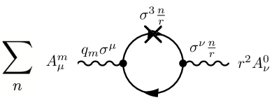
Figure 2: One-loop diagram with KK-states in the loop generating the 3D Chern-Simons level $\Theta_{0m}$.

We also introduced the momentum $k^{3}$ along the circle that is quantized as $k^{3}=\frac{n}{r}$. This gives a qualitative idea of the 3D vertex rules, however, we refer to the remainder of this section for a more thorough derivation.

The background field $r$ acts like a mass term and together with the fact that only KK-states are charged under the graviphoton, this enforces that all KK-states of the 4D massless charged fermions run in the loop. Thus, effectively we obtain infinitely many one loop diagrams, one for each KK-state, with only two external lines, namely the Abelian gauge field $A^{m}_{\mu}$ and the graviphoton $A^{0}_{\mu}$. Each single of these infinitely many loop-diagrams is of the form of the loop-diagrams considered in [64, 65, 66]. Thus, it is clear that a 3D Chern-Simons term of the form (66) is induced from the 4D mixed anomaly. The main subtlety that remains is to evaluate the infinite sum over KK-states appropriately. This sum has to be regularized by zeta function regularization and will precisely account for the prefactor in (66).

We conclude this diagrammatic discussion by excluding further 3D Chern-Simons terms by a similar logic. As can be seen from the comparison to 4D anomaly graphs, neither the Chern-Simons level $\Theta_{00}$, nor the levels $\Theta_{0i}$ can be induced at one loop. This is clear since the former would arise from the dimensional reduction of the gravitational anomaly, that is identically zero in 4D, and the latter from the mixed non-Abelian-gravitational anomaly, i.e. either $\text{tr}R^{2}\text{tr}F$ or $\text{tr}R\text{tr}F^{2}$. However, these are identically zero by $\text{tr}F=0$ due to the traceless condition of the generators of the non-Abelian gauge group in $G$ respectively the reality of the representations of the 4D Lorentz group implying $\text{tr}R=0$. The vanishing of $\Theta_{00}$ and $\Theta_{0i}$ can also be inferred directly in the 3D effective theory. For example, for $\Theta_{00}$ one can invoke a similar argument to the one of section 4.1, namely that all Kaluza-Klein modes pairwise cancel because of the sign- function in the loop-correction (60).

Let us now come to the quantitative discussion and the derivation of the Chern-Simons levels (66). The Kaluza-Klein ansatz for the 4D metric on $\mathbb{R}^{(1,2)}\times S_{r}^{1}$ takes the form

$$g^{(4)}_{MN}(x^{\mu},y)=\begin{pmatrix}g_{\mu\nu}+r^{2}A^{0}_{\mu}A^{0}_{\nu}&-r^{2}A^{0}_{\mu}\\ -r^{2}A^{0}_{\nu}&r^{2}\end{pmatrix}$$ (68)

where $y$ denotes an angular coordinate of period $2\pi$, that is related to the coordinate on the circle of radius $r$ by $ry$ and $M,N$ denote 4D Minkowski indices for the following discussion to avoid confusion. We denote the 3D Minkowski coordinates by $x^{\mu}$ and introduced the 3D metric $g_{\mu\nu}$ and the graviphoton $A_{\mu}^{0}$. For simplicity we assume no dynamics of the radial mode $r$, i.e. $r$ is a constant. We note that the reduction ansatz (68) implies the vielbein

$$e^{a}=\tilde{e}^{a}_{\mu}dx^{\mu}\,,\quad e^{3}=r(dy-A^{0}_{\mu}dx^{\mu})\,,$$ (69)

where we indicated a split $e_{M}^{A}=(e_{M}^{a},e_{M}^{3})$ of the 4D vierbein $e_{M}^{A}$, $A=0,\ldots,3$ into the 3D dreibein $e_{\mu}^{a}$, $a=0,1,2$, and a 3D one-form $e^{3}$. For completeness we introduce the inverse metric $g_{(4)}^{MN}$ and the inverse vierbein $e_{A}^{M}=e_{AN}g_{(4)}^{NM}$ reading

$$g_{(4)}^{MN}=\begin{pmatrix}g^{\mu\nu}&(A^{0})^{\mu}\\ (A^{0})^{\nu}&\frac{1}{r^{2}}+A^{0}_{\kappa}(A^{0})^{\kappa}\end{pmatrix}\,,\qquad e_{a}=\tilde{e}^{\nu}_{a}\frac{\partial}{\partial x^{\nu}}+\tilde{e}_{a}^{\nu}A^{0}_{\nu}\frac{\partial}{\partial y}\,,\quad e_{3}=\frac{1}{r}\frac{\partial}{\partial y}$$ (70)

where we raise and lower the indices $A$ and $a$ by the flat metric.

Next we specify the reduction ansatz for the 4D gauge theory. We start with vectors $A_{\mu}$ with KK-ansatz

$$A(x^{\mu},y)=A_{\mu}dx^{\mu}+\zeta r(dy-A^{0}_{\mu}dx^{\mu})=A_{\mu}dx^{\mu}+\zeta e^{3}\,,$$ (71)

where $\zeta$ denotes the adjoint valued scalar in 3D. Note that (68) and (71) imply that both $\zeta$ and $A^{0}$ have mass-dimension one by noting that $dy$ and the 3D metric have mass-dimension zero. For 4D fermions $\Psi$ charged under the 4D $U(1)$-gauge symmetries, we specify their KK-ansatz as

$$\Psi(x,y)=\sum_{n}\Psi_{n}(x)e^{iyn}\,.$$ (72)

The KK-tower of these states will be running in the loop and generate the Chern-Simons term $\Theta_{0m}$ as we will show next. It is interesting to note that while $T_{\alpha}$ transforms under the $U(1)$ as dictated by the gauge covariant derivative (46) the fermionic partners will have an ordinary derivative [68], $D_{M}=\partial_{M}$.

Considering massless 4D fermions the only terms in the 4D effective theory for the fermions $\Psi$ that are relevant for our discussion are the kinetic term. In the UV and considering a single fermion for simplicity this is the standard kinetic term for a Weyl fermion reading

$$\mathcal{L}_{\text{Weyl}}^{(4)}=-\frac{i}{\kappa_{4}^{2}}\bar{\Psi}\sigma^{A}e_{A}^{M}D_{M}\Psi\,,$$ (73)

where $D_{M}=\partial_{M}+iA_{M}$ is the 4D covariant derivative, $\sigma^{A}=(-\mathbf{1},\sigma^{i})$ and $\kappa_{4}^{2}$ the 4D Planck mass. We use (70), (71) and (72) to reduce this to three dimensions. After integration over $y$ we obtain

$$\mathcal{L}_{\text{KK}}^{(3)}=\sum_{n=-\infty}^{\infty}\left[-i\bar{\Psi}_{n}\sigma^{a}\tilde{e}^{\mu}_{a}\mathcal{D}_{\mu}\Psi_{n}+\bar{\Psi}_{n}\sigma^{3}(\frac{n}{r}+q\cdot\zeta)\Psi_{n}\right]\,,$$ (74)

where we used the shorthand notation (59). Furthermore, we have assumed in addition that we are readily on the 3D Coulomb branch by switching on VEVs for the scalars $\zeta$ along the Cartan directions of $G$ breaking it into its maximal torus $U(1)^{\text{rank}(G)}$. The $U(1)$-charges under the remaining massless gauge fields on the Coulomb branch $A^{\Lambda}$ are denoted by $q_{\Lambda}$. The covariant derivative for the KK-fermions is given by

$$\mathcal{D}_{\mu}\Psi_{n}=(\partial_{\mu}+iq_{\Lambda}A^{\Lambda}_{\mu}+inA_{\mu}^{0})\Psi_{n}\,.$$ (75)

From this we read off the 3D mass and the 3D charges of the KK-fermions that are discretely labeled by the integral momentum number $n$ along the $S^{1}$ as

$$q_{0}=n\,,\qquad m_{n}^{f}=\frac{n}{r}+q^{f}\cdot\zeta\,,$$ (76)

where we label by $f$ all the $U(1)$-charges in the case that we have more than one fermion. We see that the masses of the KK-states are offset from zero by the mass $m_{0}^{f}=\zeta\cdot q^{f}$ of the zero mode $\Psi_{0}$ on the Coulomb branch, see (59). The expressions (76) straightforwardly generalize for a more complicated constant background metric in the kinetic term (73) for several fermions. However, the diagram we want to compute has two vertices and two fermion propagators and the metric and normalizations drop out.

To determine the loop-induced Chern-Simons level $\Theta_{0m}$, we have to calculate the loop-diagram depicted in figure 2. As we have argued above heuristically, we have to integrate out all massive fermions coupling to $A^{0}$ and $A^{m}$. Indeed, we see from (74) that the whole KK-tower of fermions with charge and mass (76) couples and runs in the loop. The vertex rules are as anticipated in figure 2. The idea is now to apply at each KK-mass-level $m^{f}_{n}$ the general formula (60) with the replacement of $\text{sign}(\zeta\cdot q^{f})$ by $\text{sign}(m^{f}_{n})$. Then we use $q_{0}=n$ to obtain the one-loop correction to the Chern-Simons level as

$$\Theta^{\text{loop}}_{0m}=\frac{1}{2}\sum_{f}\sum_{n=-\infty}^{\infty}nq^{f}_{m}\,\text{sign}\Big{(}\zeta\cdot q^{f}+\frac{n}{r}\Big{)}\,.$$ (77)

This sum is in general divergent and can be regulated using zeta function regularization. We recall the definition of the Riemann zeta function by the Dirichlet series

$$\zeta(s)=\sum_{k=0}^{\infty}k^{-s}\,,\qquad\text{for }\ \ \text{Re}(s)>1\,,$$ (78)

In order to evaluate the infinite sum (77) we need the following identity that holds for $|x|<1$,

$$\sum_{n}n\,\text{sign}\Big{(}x+n\Big{)}=\sum_{n}n\,\text{sign}(n)=2\sum_{n=1}^{\infty}n=2\zeta(-1)=-\frac{1}{6}\,.$$ (79)

We note that the first equality holds since $x$ lies in the interval $[0,1)$ and this allows us to replace $\text{sign}(n+x)=\text{sign}(n)$. Then in the second equality we split the sum into positive and negative $n$, that yields due to the sign$(n)$ the same sum. Finally we used the well-known result $\zeta(-1)=-\frac{1}{12}$ from analytic continuation of the Riemann zeta function (78) for $\text{Re}(s)<1$.

Now we are prepared to perform the sum over $n$ in (77). We focus on each summand in the sum over fermions $f$ independently. Furthermore, we identify $x\equiv rm_{0}^{f}=r\zeta\cdot q^{f}$ in (79). We consider the effective theory in the IR at an energy scale, that is sufficiently smaller than the mass-scale $m_{\text{KK}}$ of KK-states and the mass scale $m_{0}^{f}$ on the Coulomb branch. However, in order to apply the field theory analysis of [64, 65, 66] and the result (60) the masses $m^{f}_{0}$ of the massive fermions have to be smaller than the KK mass scale $m_{\text{KK}}$ as in (62). Since the mass scale $m_{0}^{f}$ depends on the position $\zeta^{\Lambda}$ on the 3D Coulomb branch, it can be made parametrically small. In this case we can trust the loop result (60). We then have $x\equiv rm_{0}^{f}<1$ and can apply (79) to readily obtain the Chern-Simons levels as

$$\Theta^{\text{loop}}_{0m}=-\frac{1}{12}\sum_{f}q_{m}^{f}=-\frac{1}{12}\sum_{\underline{q}}n(\underline{q})q_{m}\,.$$ (80)

Here we replaced the sum over individual fermions $f$ by a sum over charges $q$ where $n(\underline{q})$ denotes their multiplicities. We note that (80) is an odd function in the charges and as a result only sensitive to the chiral index 4D $\chi(\underline{q})=n(\underline{q})-n(-\underline{q})$ since 4D vector-like pairs of fermions cancel out.

We see that (80) is precisely the mixed Abelian-gravitational anomaly on the left hand side in (16). This is what one expects since, by reversing the logic from the beginning of this section, in the limit $\zeta\rightarrow 0$ we have $x=0$ and sending $r\rightarrow\infty$ all KK-states become massless and we have to recover the 4D anomaly result.

5 Anomaly Cancellation In F-Theory

In this section we will discuss anomaly cancellation in F-theory. This involves relating, via the general formulas (13)–(16) for anomaly cancellation in section 2, the Green-Schwarz counter terms discussed in section 3.3 to the 4D chiralities obtained from 3D Chern-Simons terms following section 4. This will connect seemingly physically different object, the geometric intersections on $\hat{X}_{4}$ and flux integrals, with each other. The main challenge of this section will be to understand these relations directly from analyzing the geometrical structure of the resolution fourfold $\hat{X}_{4}$ on the one hand, and 3D Chern-Simons terms on the other hand. Anomaly cancellation in 6D F-theory compactifications has been under intense investigation as reviewed in [69].

5.1 The geometric structure of F-theory anomaly cancellation

We begin with an outline of the general geometric relations imposed on $\hat{X}_{4}$ by anomaly cancellation in F-theory. As we will argue in this section these relate intersections of resolution divisors and holomorphic curves over the matter curves $\Sigma_{\mathbf{R}}$ in the base $B_{3}$ on the one side to certain flux integrals on $\hat{X}_{4}$ on the other side. These geometric relations that we will discover by imposing 4D anomaly cancellation will be very similar to those found in 6D F-theory on Calabi-Yau threefolds [23]. The crucial point in the analysis in 4D will be the necessity of the inclusion of $G_{4}$-flux on both sides of the discovered relations.

The 4D anomaly cancellation conditions (13)–(16) can be directly translated into the geometry of the resolved fourfold $\hat{X}_{4}$. We denote the holomorphic curves in $\hat{X}_{4}$, that resolve singular elliptic fibers over codimension two in the base $B_{3}$ and that thus lie in the weight lattice of $G$, by $c$. Then, the 4D charge of a matter particle obtained from a wrapped M2-brane on $c$ under $A^{\Lambda}$ is given by

$$q_{\Lambda}=\int_{c}\omega_{\Lambda}\,.$$ (81)

This can be seen from reducing the electric coupling of the M2-brane to $C_{3}$ along $c$. Then the anomaly constraints relate sums over these holomorphic curves in the weight lattice of $G$ to certain flux integrals of $G_{4}$. It is important to emphasize that the following geometric relations only hold if the $G_{4}$-flux obeys all the conditions (47) and not for generic $G_{4}$-flux in M-theory. The anomaly cancellation conditions (13)-(15), using (81) to express the charges, then translate into

$$\frac{1}{3}\sum_{S_{\mathbf{R}}}\sum_{c\,\subset S_{\mathbf{R}}}\int_{S_{\mathbf{R}}}G_{4}\int_{c}\omega_{(\Lambda}\int_{c}\omega_{\Sigma}\int_{c}\omega_{\Gamma)} = \frac{1}{2}\int_{\hat{X}_{4}}G_{4}\wedge\omega_{\alpha}\wedge\omega_{(\Gamma}\eta^{-1\,\alpha}_{\beta}\int_{S^{\beta}}\omega_{\Lambda}\wedge\omega_{\Sigma)}$$ (82)

$$= \frac{1}{2}\int_{\hat{X}_{4}}G_{4}\wedge\pi_{*}(\omega_{(\Lambda}\wedge\omega_{\Sigma})\wedge\omega_{\Gamma)}\,,$$

where we indicate a symmetrization of indices $\Lambda$, $\Sigma$ and $\Gamma$ by $(\cdot)$. The cancellation condition (16) of the Abelian-gravitational anomaly yields the geometric relation

$$\frac{1}{3}\sum_{S_{\mathbf{R}}}\sum_{c\,\subset S_{\mathbf{R}}}\int_{S_{\mathbf{R}}}G_{4}\int_{c}\omega_{\Lambda} = \int_{\hat{X}_{4}}G_{4}\wedge\omega_{\alpha}\wedge\omega_{\Lambda}\eta^{-1\,\alpha}_{\beta}\int_{S_{\rm b}^{\beta}}c_{1}(B_{3})$$ (83)

$$= \int_{\hat{X}_{4}}G_{4}\wedge c_{1}(B_{3})\wedge\omega_{\Lambda}\,.$$

In both equations we split the sum over curves $c$ into a sum over matter surfaces $S_{\mathbf{R}}$ and a sum over curves $c$ lying inside a particular $S_{\mathbf{R}}$. In addition we used the topological metric $\eta_{\alpha}^{\ \beta}$ respectively its inverse $\eta_{\alpha}^{-1\,\beta}$ on $B_{3}$ as introduced in (36) and from the first to the second line in each equation the push-forward $\pi_{*}$ to $H^{(1,1)}(B_{3})$ defined in (52).

We can use Poincaré duality to rewrite the relation (82) and (83) more compactly in homology as intersections of divisors and holomorphic curves $c$ in the weight lattice of $G$

$$\frac{1}{3}\sum_{S_{\mathbf{R}}}\sum_{c\,\subset S_{\mathbf{R}}}(S_{\mathbf{R}}\cdot[G_{4}])(c\cdot D_{(\Lambda})(c\cdot D_{\Sigma})(c\cdot D_{\Gamma)}) = \frac{1}{2}[G_{4}]\cdot D_{(\Gamma}\cdot\pi_{*}(D_{\Lambda}\cdot D_{\Sigma)})\ ,$$ (84)

$$\frac{1}{3}\sum_{S_{\mathbf{R}}}\sum_{c\,\subset S_{\mathbf{R}}}(S_{\mathbf{R}}\cdot[G_{4}])(c\cdot D_{\Lambda}) = [G_{4}]\cdot[c_{1}(B_{3})]\cdot D_{\Lambda}\,,$$

where we again symmetrized the indices $\Lambda$, $\Sigma$ and $\Gamma$.

Both (82) and the first equation contains of (84) capture all three different types of gauge anomalies, i.e. the purely Abelian as well as non-Abelian anomalies and the mixed Abelian-non-Abelian anomalies. This can be seen by choosing $\Gamma,\Sigma,\Lambda$ as the indices of the Cartan divisors $D_{i_{I}}$ of $G_{(I)}$ and noting that the right hand side vanishes because of $\Theta_{i\alpha}=0$ in (47) yielding the purely non-Abelian anomaly condition (13). The mixed Abelian-non-Abelian anomaly (15) is obtained by choosing $\Gamma,\Sigma,\Lambda=i,j,m$. In order to see a matching of the Lie algebra structure we expand following [23] the Cartan generators in the GS-terms (11) involving $\text{tr}(F^{I}\wedge F^{I})$ in a coroot basis $\mathcal{T}_{i_{I}}$. Since the anomalies have to hold for all Cartan generators and exploiting $\frac{1}{\lambda_{I}}\text{tr}(\mathcal{T}_{i_{I}}\mathcal{T}_{j_{I}})=\mathcal{C}^{(I)}_{i_{I}j_{I}}$ in the GS-terms we obtain a match with the right hand side of (82), (84), where we employ (29) . The purely Abelian anomaly (14) is manifest for the choice $\Gamma,\Sigma,\Lambda=m,n,k$. The second equation summarizes all mixed Abelian-gravitational anomalies (16) as is evident by choosing $\Lambda=m$.

As we have noted already in the introduction the conditions (84) might generally hold also for $G_{4}$-flux that are not wedges of two two-forms as in (43). These more general $G_{4}$-flux can correspond to seven-brane fluxes trivial in the ambient space. For these fluxes the right-hand side of (84) induced by the gaugings vanishes and the left side might pose a non-trivial constraint on the spectrum.

5.2 The structure of F-theory fluxes and Green-Schwarz terms

Next we discuss the general structure of the $G_{4}$-flux obeying the F-theory constraints (47). A very general, presumably the most general, vertical $G_{4}$-flux on $\hat{X}_{4}$ that can meet all conditions listed in section 3.2 takes the form

$$G_{4}=\widehat{G}_{4}+F^{(m)}\wedge\omega_{m}\,.$$ (85)

Here the first term $\widehat{G}_{4}$ denotes a non-Abelian flux related to the non-Abelian gauge groups $G_{(I)}$. It only involves the two-forms $\omega_{i},\omega_{\alpha},\omega_{0}$ introduced in (21). The second part are Abelian fluxes that are of the form of wedge products of a two-form $F^{(m)}$ in $B_{3}$ with each $\omega_{m}$ dual to the $U(1)$-Cartan divisors $D_{m}$ in (21). These fluxes can be thought of as the lift of internal world-volume fluxes $F^{(m)}$ on each $U(1)$ seven-brane to $G_{4}$-flux. The fluxes $F^{(m)}$ being $(1,1)$-forms on $B_{3}$ can be expanded, after introducing in general arbitrary flux numbers $f^{(m)\alpha}$, as

$$F^{(m)}=f^{(m)\alpha}\,\omega_{\alpha}\,.$$ (86)

The validity of the generic splitting (85) of $G_{4}$ into Abelian and non-Abelian fluxes can be motivated by moving in the complex structure moduli space of the Calabi-Yau fourfold. For this argument let us begin with a fourfold $\hat{Y}_{4}$ yielding a purely non-Abelian gauge group $G_{(I)}$ without any $U(1)$-factors. Then only the first flux in (85) is present, of which we assume that it obeys all consistency conditions (47) on $\hat{Y}_{4}$. Upon specializing the complex structure of $\hat{Y}_{4}$ we can unhiggs a number of $U(1)$ symmetries by forming and resolving a singularities in $\hat{Y}_{4}$. This leads to a new fourfold $\hat{X}_{4}$ with extra divisors $D_{m}$. Then we can just pull-back the non-Abelian flux $\widehat{G}_{4}$ from $\hat{Y}_{4}$ to $\hat{X}_{4}$ and obtain, by virtue of the second and third equation in (38), a valid flux that we again denoted by $\widehat{G}_{4}$. This pull-back flux is still the most general non-Abelian flux $\widehat{G}_{4}$ we can construct on $\hat{X}_{4}$, since $\widehat{G}_{4}$ by definition involves only the $\omega_{i}$, $\omega_{\alpha}$ and $\omega_{0}$ and since in the transition from $\hat{Y}_{4}$ to $\hat{X}_{4}$ no any new Cartan divisors $D_{i}$ nor new base divisors $D_{\alpha}$ were induced. Thus, new fluxes on $\hat{X}_{4}$ that were not available on $\hat{Y}_{4}$ are of the form $F^{(m)}\wedge\omega_{m}$, where $F^{(m)}$ is a general two-form on $B_{3}$ as we will see below.

5.2.1 Non-Abelian fluxes only

We start by working out the conditions imposed by (47) on the non-Abelian flux $\widehat{G}_{4}$ in (85) as well as the gaugings induced by it. We expand $\widehat{G}_{4}$ that in a basis of cohomology of $H^{4}_{V}(\hat{X}_{4})$ as

$$\widehat{G}_{4}=N^{ij}\,\omega_{i}\wedge\omega_{j}+f^{i\alpha}\,\omega_{i}\wedge\omega_{\alpha}+\tilde{N}_{\alpha}\,\tilde{\omega}^{\alpha}+N^{\alpha}\,\omega_{0}\wedge\omega_{\alpha}\,,$$ (87)

where the $\tilde{\omega}^{\alpha}$ as before denote pull-backs from $H^{4}(B_{3})$. The coefficients $f^{i\alpha}$ have the interpretation of a seven-brane two-form flux $F_{2}^{i}$ in the direction of the i-th Cartan generator of $G$. The fluxes $N^{ij}$ are non-Abelian in nature as they are associated to products of two Cartan divisors.

With the expansion (87) of $\widehat{G}_{4}$ we readily evaluate the constraints (47). Employing the conditions (39), (41), (29), (38) and (25) we obtain after some algebra the following,

$$\Theta_{00} = K^{\alpha}K^{\beta}\Theta_{\alpha\beta}\,,\qquad\qquad\qquad\qquad\quad\ \ \,\Theta_{0\alpha}=\frac{1}{2}(\tilde{N}_{\alpha}+N^{\gamma}K^{\beta}\mathcal{K}_{\alpha\beta\gamma}-K^{\beta}\Theta_{\alpha\beta})\,,$$

$$\Theta_{0\Lambda} = -\frac{1}{2}K^{\alpha}\Theta_{\alpha\Lambda}\,,\qquad\qquad\qquad\qquad\quad\ \ \Theta_{\alpha\beta}=\frac{1}{2}(N^{\gamma}-N^{ij}C_{ij}^{\gamma})\mathcal{K}_{\alpha\beta\gamma}\,,$$

$$\Theta_{\alpha i} = \frac{1}{2}(N^{j_{1}j_{2}}\mathcal{K}_{ij_{1}j_{2}\alpha}-f^{j\beta}C_{ij}^{\gamma}\mathcal{K}_{\alpha\beta\gamma})\,,\qquad\quad\Theta_{\alpha m}=\frac{1}{2}N^{ij}\mathcal{K}_{ijm\alpha}\,,$$

$$\Theta_{ij} = \frac{1}{2}(N^{i_{1}i_{2}}\mathcal{K}_{i_{1}i_{2}ij}+f^{i_{1}\alpha}\mathcal{K}_{i_{1}ij\alpha}-\tilde{N}_{\alpha}C_{ij}^{\alpha})\,,\,\,\,\Theta_{im}=\frac{1}{2}(N^{i_{1}i_{2}}\mathcal{K}_{i_{1}i_{2}im}+f^{j\alpha}\mathcal{K}_{ijm\alpha})\,,$$

$$\Theta_{mn} = \frac{1}{2}(N^{ij}\mathcal{K}_{ijmn}+f^{i\alpha}\mathcal{K}_{imn\alpha}-\tilde{N}_{\alpha}b_{mn}^{\alpha})\,.$$ (88)

Here we used the definitions (20), (49), (50) and $\mathcal{K}_{\alpha\beta\gamma}$ denotes the triple intersections on $B_{3}$ introduced in (26) and the $K^{\alpha}$ were defined by the expansion $c_{1}(B_{3})=-K^{\alpha}\omega_{\alpha}$. We also introduced the shorthand notation $C^{\gamma}_{ij}=C_{ij}^{(I)}b^{\gamma}_{I}$.

Indeed, we can solve the constraints (47) explicitly using the expressions (5.2.1). We obtain three sets of conditions from $\Theta_{\alpha\beta}=\Theta_{0\alpha}=\Theta_{\alpha i}=0$ that we solve to determine the flux numbers $N^{\alpha}$, $\tilde{N}_{\alpha}$ and $f^{i\alpha}$ in terms of the $N^{ij}$,

$$N^{\alpha}=N^{ij}C_{ij}^{\alpha}\,,\qquad\tilde{N}_{\gamma}=-\frac{1}{2}(N^{\gamma}+N^{ij}C_{ij}^{\gamma})K^{\beta}\mathcal{K}_{\alpha\beta\gamma}=-N^{ij}C_{ij}^{\gamma}K^{\beta}\mathcal{K}_{\alpha\beta\gamma}\,,$$

$$f^{i\alpha}=N^{i_{1}i_{2}}\mathcal{K}_{i_{1}i_{2}j\alpha}(C^{-1}_{(I)})^{ji}\mathcal{K}_{S_{(I)}^{\rm b}}^{\beta\alpha}\,.$$ (89)

Here we have introduced the inverse $\mathcal{K}_{S_{(I)}^{\rm b}}^{\beta\alpha}$ of the intersection form on the seven-brane divisor $S^{A}_{\rm b}$ as well as the inverse of the corresponding Cartan matrix $C^{-1}_{(I)}$.

It is satisfying to see that $\Theta_{0m}=-\frac{1}{2}K^{\alpha}\Theta_{\alpha m}$ is implied by (5.2.1). Thus, $\Theta_{0m}$ is precisely the coefficient of the Green-Schwarz counter term relevant for the cancellation of mixed Abelian- gravitational anomalies in (16) respectively (83). This is precisely what we expect from the discussion of section 4.2 where we related the Chern-Simons level $\Theta_{0m}^{\text{loop}}$ induced by loops of KK- fermions to precisely the mixed anomalies. As we argued there further, the matching of the 3D Chern-Simons levels $\Theta_{0m}\equiv\Theta_{0m}^{\text{loop}}$ by M-/F-theory duality (19) is a prove of the 4D anomaly cancellation condition.

Before switching to the discussion of Abelian fluxes let us conclude by mentioning that by virtue of section 4 the flux integrals $\Theta_{\Sigma\Lambda}$ in the next to last and last line in (5.2.1) encode the 4D chiralities. By means of (5.2.1) the chiralities only depend on the flux numbers $N^{ij}$. It would be interesting to explicitly express these in terms of the $N^{ij}$.

5.2.2 Inclusion of Abelian fluxes

We begin by checking that Abelian fluxes of the form alluded to in (85) can be added to a given non-Abelian flux $\widehat{G}_{4}$. For this we check that fluxes of the form $F^{(m)}\wedge\omega_{m}$ with $F^{(m)}$ obtained from elements in $H^{(1,1)}(B_{3})$ obey all constraints in (47).

As before we work out explicitly the flux integrals $\Theta_{AB}$. Using again the intersections (38) and (39), (41) as well as the shifted form $\tilde{\omega}_{0}$ defined in (24) we obtain

$$\Theta_{00}=\Theta_{0\alpha}=\Theta_{0i}=\Theta_{\alpha\beta}=\Theta_{\alpha i}=0\,,\quad$$ (90)

and

$$\Theta_{0m}=-\frac{1}{2}K^{\alpha}\Theta_{\alpha m}\ ,\qquad\quad\Theta_{\alpha m}=-\frac{1}{2}f^{(n)\beta}b_{nm}^{\gamma}\mathcal{K}_{\alpha\beta\gamma}\ ,$$

$$\Theta_{ij}=\frac{1}{2}f^{(m)\alpha}\,\mathcal{K}_{\alpha mij}\ ,\quad\Theta_{im}=\frac{1}{2}f^{(n)\alpha}\mathcal{K}_{\alpha mnj}\ ,\quad\Theta_{mn}=\frac{1}{2}f^{(p)\alpha}\mathcal{K}_{\alpha pmn}\ .$$ (91)

We see that all conditions (47) are automatically obeyed. We note that we again have $\Theta_{0m}=-\frac{1}{2}K^{\alpha}\Theta_{\alpha m}$ in agreement with the discussion in section 4.2, as in the non-Abelian case discussed above. As expected the new fluxes contribute to the $\Theta_{\Sigma\Lambda}$ and thus will generate additional 4D chiralities.

6 Anomalies and GS-terms in Type IIB Orientifolds

In this section we analyze the connection of F-theory anomaly cancellation to anomaly cancellation in Type IIB orientifold setups at weak string coupling. We first recall anomaly cancellation for compactifications with D7-branes and O7-planes in subsection 6.1 by largely following [20]. The discussion of anomalies and their cancellation in Type II orientifold setups has been studied significantly in the past, as can be found in the reviews [16, 17, 18, 19]. This comparison to F-theory is performed in subsection 6.2, by relating the gaugings and Green-Schwarz counter terms of both setups. We discuss the complications arising due to additional ‘geometrically massive’ $U(1)$ gauge symmetries that are present in orientifold setups but integrated out in F-theory. A detailed comparison $G_{4}$-flux in M-theory dual to F-theory compactifications with $SU(N)$ and $SU(N)\times U(1)$ and D7-brane fluxes in the Type IIB orientifold limit has been addressed in [14].

6.1 Anomaly cancellation in Type IIB orientifolds

We begin with a review of anomaly cancellation in Type IIB orientifolds with intersecting D7-branes. We consider Abelian or non-Abelian D7-branes on divisors $S^{\rm IIB}_{(\mathcal{A})}$ in the orientifold covering space $Y_{3}$ and denote the orientifold images of these D7-brane divisors by $S^{\rm IIB}_{(\mathcal{A}^{\prime})}$. The orientifold planes are located at the fix-point set of the orientifold involution denoted by $S^{\rm O7}$. The number of D7-branes on a stack are denoted by $N_{\mathcal{A}}$. This includes cases where $N_{\mathcal{A}}=1$ yielding a D7-brane with a $U(1)$ gauge group. In the following we will only focus on $U(N_{\mathcal{A}})$ groups for simplicity, such that the 4D gauge group is given by

$$G_{\rm ori}=U(N_{1})\times\ldots\times U(N_{{\widehat{n}_{G}}})\ ,\qquad{\mathcal{A}}=1,\dots,\widehat{n}_{G}\ .$$ (92)

The cases $SO(N_{I})$ and $Sp(N_{I})$ should work out similarly and it would be interesting to perform such an analysis using F-theory.

The Type IIB orientifold matter spectrum arises from strings stretching between D7-branes. Four representations are present: (1) the bi-fundamental representation $\mathbf{F}_{\bar{\mathcal{A}}\mathcal{B}}=(\bar{N}_{\mathcal{A}},N_{\mathcal{B}})$ corresponding to strings stretching from a D7-brane on $S_{(\mathcal{A})}^{\rm D7}$ to a D7-brane on $S_{(\mathcal{B})}^{\rm D7}$ with $\mathcal{A}\neq\mathcal{B}$; (2) the bi-fundamental representation $\mathbf{F}_{\mathcal{A}\mathcal{B}}=(N_{\mathcal{A}},N_{\mathcal{B}})$ for strings stretching between $S_{(\mathcal{A}^{\prime})}^{\rm D7}$ and $S_{(\mathcal{B})}^{\rm D7}$ with $\mathcal{A}\neq\mathcal{B}$; (3) the symmetric representation $\mathbf{S}_{\mathcal{A}}$, (4) the anti-symmetric representation $\mathbf{A}_{\mathcal{A}}$. The latter two arise from strings stretching between the brane and its orientifold image. For evaluating the anomaly cancellation conditions it will be crucial to give the $U(1)$-charges $q_{\mathcal{A}}(\mathbf{R})$ under the $\mathcal{A}$th $U(1)$ in (92) of the various representations. Together with the dimension of the representations they are summarized in Table 1.

The chiral indices in the orientifold setup are denoted by $\chi(\mathbf{R})$. For the intersecting D7-brane setup one has the relations

$$\chi(\mathbf{F}_{\mathcal{A}\mathcal{B}})=\chi(\mathbf{F}_{\mathcal{B}\mathcal{A}})\ ,\quad\chi(\mathbf{F}_{\bar{\mathcal{A}}\mathcal{B}})=-\chi(\mathbf{F}_{\bar{\mathcal{B}}\mathcal{A}})\ ,\quad\chi(\mathbf{F}_{\bar{\mathcal{A}}\mathcal{A}})=0\,,\quad\chi(\mathbf{F}_{\mathcal{A}\mathcal{A}})=\chi(\mathbf{S}_{\mathcal{A}})+\chi(\mathbf{A}_{\mathcal{A}})\,.$$ (93)

The first condition is trivially true since exchanging brane and image, which is a symmetry of the theory, exchanges the fundamental representations. The second condition uses the fact that the bi-fundamental $(\bar{N}_{\mathcal{A}},N_{\mathcal{B}})$ is the complex conjugate of $(N_{\mathcal{A}},\bar{N}_{\mathcal{B}})$ and the chiral index changes sign under the exchange of a representation and its complex conjugate. The third equality is true since since the representation $\mathbf{F}_{\bar{\mathcal{A}}\mathcal{A}}$ is real and the last equality makes use of the group theoretical decomposition $N_{\mathcal{A}}\otimes N_{\mathcal{A}}=\mathbf{S}_{\mathcal{A}}\oplus\mathbf{A}_{\mathcal{A}}$. To simplify our notation we will introduce the abbreviations

$$\chi_{\mathcal{A}\mathcal{B}}=\chi(\mathbf{F}_{\mathcal{A}\mathcal{B}})\ ,\qquad\chi_{\bar{\mathcal{A}}\mathcal{B}}=\chi(\mathbf{F}_{\bar{\mathcal{A}}\mathcal{B}})\ ,\qquad\chi_{(\mathcal{A})}=\chi(\mathbf{S}_{\mathcal{A}})\ ,\qquad\chi_{[\mathcal{A}]}=\chi(\mathbf{A}_{\mathcal{A}})\ .$$ (94)

The chiralities in Type IIB are calculated explicitly from a simple index depending on the D7-brane flux. In the following we will focus on D7-branes with $U(1)$-fluxes $\mathcal{F}^{\mathcal{A}}$ only, which are a non-trivial background on $S^{\rm IIB}_{\mathcal{A}}$ in the $U(1)$-directions of (92). The indices then read

$$I_{\mathcal{A}\mathcal{B}}=\int_{S^{\rm IIB}_{(\mathcal{A})}\cdot S^{\rm IIB}_{(\mathcal{B})}}(\mathcal{F}^{\mathcal{A}}-\mathcal{F}^{\mathcal{B}})\,$$ (95)

for two D7-brane divisors $S^{\rm IIB}_{(\mathcal{A})},$ $S^{\rm IIB}_{(\mathcal{B})}$ with their intersection denoted by $S^{\rm IIB}_{(\mathcal{A})}\cdot S^{\rm IIB}_{(\mathcal{B})}$. For convenience we have set the string length $\ell_{s}=1$. In terms of these indices the chiralities are given by

$$\chi_{\bar{\mathcal{A}}\mathcal{B}} = I_{\mathcal{A}\mathcal{B}}\,,\qquad\chi_{\mathcal{A}\mathcal{B}}=I_{\mathcal{A}^{\prime}\mathcal{B}}\,,$$ (96)

$$\chi_{(\mathcal{A})} = \tfrac{1}{2}(I_{\mathcal{A}^{\prime}\mathcal{A}}-2I_{O7\mathcal{A}})\,,\quad\chi_{[\mathcal{A}]}=\tfrac{1}{2}(I_{\mathcal{A}^{\prime}\mathcal{A}}+2I_{O7\mathcal{A}})\,.$$

Here $\mathcal{A}^{\prime}$ denotes the orientifold image of a divisor $S^{\rm IIB}_{(\mathcal{A})}$ and $I_{O7\mathcal{A}}$ is obtained from (95) by using the orientifold divisor $S_{\rm O7}$ and noting that the are no fluxes on an O7-plane. We note that from (96) and the symmetry properties of (95) we immediately obtain the relations (93), where we here and in the following have to make use of

$$\mathcal{F}^{\mathcal{A}^{\prime}}\wedge[S^{\rm IIB}_{\mathcal{A}^{\prime}}]=-\sigma^{*}(\mathcal{F}^{\mathcal{A}}\wedge[S^{\rm IIB}_{\mathcal{A}}])\,,\qquad A^{\mathcal{A}}_{U(1)}=-\sigma^{*}A^{\mathcal{A}^{\prime}}_{U(1)}\,.$$ (97)

The map $\sigma$ denotes the orientifold involution and $A^{\mathcal{A}}_{U(1)}$ are the $U(1)$-gauge fields in the setup.

$\mathbf{R}$	rep.	$U(1)_{\mathcal{C}}$-charge	$\text{dim}(\mathbf{R})$	$\quad V(\mathbf{R})\quad$	$U(\mathbf{R})$	$\chi(\mathbf{R})$
$\mathbf{F}_{\bar{\mathcal{A}}\mathcal{B}}$	$(\bar{N}_{\mathcal{A}},N_{\mathcal{B}})_{\underline{q}}$	$(\underline{q})_{\mathcal{C}}=-\delta_{\mathcal{C}\mathcal{A}}+\delta_{\mathcal{C}\mathcal{B}}$	$N_{\mathcal{A}}N_{\mathcal{B}}$	$(-1,1)$	$(1,1)$	$\chi_{\bar{\mathcal{A}}\mathcal{B}}$
$\mathbf{F}_{\mathcal{A}\mathcal{B}}$	$(N_{\mathcal{A}},N_{\mathcal{B}})_{\underline{q}}$	$(\underline{q})_{\mathcal{C}}=\delta_{\mathcal{C}\mathcal{A}}+\delta_{\mathcal{C}\mathcal{B}}$	$N_{\mathcal{A}}N_{\mathcal{B}}$	$(1,1)$	$(1,1)$	$\chi_{\mathcal{A}\mathcal{B}}$
$\mathbf{S}_{\mathcal{A}}$	$\text{Sym}(N_{\mathcal{A}})_{\underline{q}}$	$(\underline{q})_{\mathcal{C}}=2\delta_{\mathcal{C}\mathcal{A}}$	$\tfrac{1}{2}N_{\mathcal{A}}(N_{\mathcal{A}}+1)$	$N_{A}+4$	$N_{A}+2$	$\chi_{(\mathcal{A})}$
$\mathbf{A}_{\mathcal{A}}$	$\Lambda^{2}(N_{\mathcal{A}})_{\underline{q}}$	$(\underline{q})_{\mathcal{C}}=2\delta_{\mathcal{C}\mathcal{A}}$	$\tfrac{1}{2}N_{\mathcal{A}}(N_{\mathcal{A}}-1)$	$N_{A}-4$	$N_{A}-2$	$\chi_{[\mathcal{A}]}$

Table 1: A list of the matter representations arising from intersecting D7- branes. The second column denotes the representations of $SU(N_{\mathcal{A}})\times SU(N_{\mathcal{B}})\times U(1)^{\hat{n}_{G}}$ respectively of $SU(N_{\mathcal{A}})\times U(1)^{\hat{n}_{G}}$ and the third column denotes the charges under the $\mathcal{C}$th $U(1)$. Finally we summarize the dimension of $\mathbf{R}$ in the fourth, the values of the cubic Casimir and the index in (18) in the fifth respectively sixth columns and the chiral indices in the last.

Next we evaluate the anomalies on the left-hand side of (13)-(16) for the 4D orientifold theory. One evaluates for the weak coupling representations employing the last relation in (93) and Table 1 that

$$\text{tr}_{\mathbf{f}}(F^{\mathcal{A}})^{3}: A^{F^{3}}_{\mathcal{A}}=\sum_{\mathcal{C}\neq\mathcal{A}}N_{\mathcal{C}}\big{(}\chi_{\bar{\mathcal{C}}\mathcal{A}}+\chi_{\mathcal{C}\mathcal{A}}\big{)}+(N_{\mathcal{A}}+4)\chi_{(\mathcal{A})}+(N_{\mathcal{A}}-4)\chi_{[\mathcal{A}]}\,,$$

$$F^{\mathcal{A}}_{U(1)}(F^{\mathcal{B}}_{U(1)})^{2}: \tfrac{1}{2}N_{\mathcal{A}}\big{[}N_{\mathcal{B}}\big{(}\chi_{\bar{\mathcal{B}}\mathcal{A}}+\chi_{\mathcal{B}\mathcal{A}}\big{)}(1-\delta_{\mathcal{A}\mathcal{B}})$$

$$+\tfrac{1}{3}\delta_{\mathcal{A}\mathcal{B}}\big{(}\sum_{\mathcal{C}\neq\mathcal{A}}N_{\mathcal{C}}\big{(}\chi_{\bar{\mathcal{C}}\mathcal{A}}+\chi_{\mathcal{C}\mathcal{A}}\big{)}+4(N_{\mathcal{A}}+1)\chi_{(\mathcal{A})}+4(N_{\mathcal{A}}-1)\chi_{[\mathcal{A}]}\big{)}\big{]}$$

$$=\tfrac{1}{2}N_{\mathcal{A}}\big{[}N_{\mathcal{B}}\big{(}\chi_{\bar{\mathcal{B}}\mathcal{A}}+\chi_{\mathcal{B}\mathcal{A}}\big{)}+\tfrac{1}{3}\delta_{\mathcal{A}\mathcal{B}}A^{F^{3}}_{\mathcal{A}}\big{]}\,,$$

$$F^{\mathcal{A}}_{U(1)}\text{tr}_{\mathbf{f}}(F^{\mathcal{B}})^{2}: \tfrac{1}{2}\big{[}N_{\mathcal{A}}\big{(}\chi_{\bar{\mathcal{B}}\mathcal{A}}+\chi_{\mathcal{B}\mathcal{A}}\big{)}(1-\delta_{\mathcal{A}\mathcal{B}})+\delta_{\mathcal{A}\mathcal{B}}\big{(}\sum_{\mathcal{C}\neq\mathcal{A}}N_{\mathcal{C}}\big{(}\chi_{\bar{\mathcal{C}}\mathcal{A}}+\chi_{\mathcal{C}\mathcal{A}}\big{)}$$

$$+2(N_{\mathcal{A}}+2)\chi_{(\mathcal{A})}+2(N_{\mathcal{A}}-2)\chi_{[\mathcal{A}]}\big{)}\big{]}=\tfrac{1}{2}\big{[}N_{\mathcal{A}}\big{(}\chi_{\bar{\mathcal{B}}\mathcal{A}}+\chi_{\mathcal{B}\mathcal{A}}\big{)}+\delta_{\mathcal{A}\mathcal{B}}A^{F^{3}}_{\mathcal{A}}\big{]}\,,$$

$$F^{\mathcal{A}}_{U(1)}\text{tr}R^{2}: \tfrac{1}{48}N_{\mathcal{A}}\Big{[}A^{F^{3}}_{\mathcal{A}}-3\chi_{(\mathcal{A})}+3\chi_{[\mathcal{A}]}\Big{]}=\tfrac{1}{48}N_{\mathcal{A}}\Big{[}A^{F^{3}}_{\mathcal{A}}+6I_{O7\mathcal{A}}\Big{]}\ .$$ (100)

Here $F^{\mathcal{A}}$ denotes the field strength of $SU(N_{\mathcal{A}})$ and $F^{\mathcal{A}}_{U(1)}$ are the $U(1)$ field strengths of the Abelian factors appearing in (92). Note that the contribution $\delta_{\mathcal{A}\mathcal{B}}$ in the second and third condition arises from bi-fundamental matter from all intersections with D7-branes with the $\mathcal{A}$-stack together with the symmetric and anti-symmetric representations arising from the $\mathcal{A}$-stack itself. We have conveniently written the result using $A^{F^{3}}_{\mathcal{A}}$.

These anomalies are canceled by a GS-mechanism in 4D when imposing D7-brane and D5-brane tadpole cancellation. For general Type IIB Calabi-Yau orientifold setups with D7-branes this has been shown in [20]. Since $\text{tr}_{\mathbf{f}}(F^{\mathcal{A}})^{3}$ is non-factorizable one has

$$\text{D7-/D5-tadpole cancellation}\qquad\Rightarrow\qquad A^{F^{3}}_{\mathcal{A}}=0\ .$$ (101)

The remaining conditions then read

$$F^{\mathcal{A}}_{U(1)}(F^{\mathcal{B}}_{U(1)})^{2} :\quad \tfrac{1}{2}N_{\mathcal{A}}N_{\mathcal{B}}\,\big{[}I_{\mathcal{B}\mathcal{A}}+I_{\mathcal{B}^{\prime}\mathcal{A}}\big{]}\,,$$ (102)

$$F^{\mathcal{A}}_{U(1)}\text{tr}_{\mathbf{f}}(F^{\mathcal{B}})^{2} :\quad \tfrac{1}{2}N_{\mathcal{A}}\,\big{[}I_{\mathcal{B}\mathcal{A}}+I_{\mathcal{B}^{\prime}\mathcal{A}}\big{]}\,,$$

$$F^{\mathcal{A}}_{U(1)}\text{tr}R^{2} :\quad \tfrac{1}{8}N_{\mathcal{A}}\,I_{O7\mathcal{A}}\ ,$$

where we have used the relations (96) and (97). This concludes the evaluation of the one-loop anomaly.

Next we will recall the derivation of the gaugings and Green-Schwarz counter terms. There are two different types of axions relevant in the Green-Schwarz mechanism in Type IIB orientifolds. Firstly, there are orientifold-even axions $\rho_{\alpha}$ arising from the expansion of the R–R-form $C_{4}$ into a basis of $H^{4}_{+}(Y_{3})$. Secondly, there are orientifold-odd axions in the expansion of the R–R-form $C_{2}$ into a basis of $H^{2}_{-}(Y_{3})$. They appear in the Green-Schwarz-terms of Type IIB as

$$S_{\rm GS}^{(4)}=-\frac{1}{4}\int(b^{\alpha}_{\mathcal{A}}\rho_{\alpha}+b_{a\,\mathcal{A}}c^{a})\text{tr}(F^{\mathcal{A}}\wedge F^{\mathcal{A}})+(b^{\alpha}_{\mathcal{A}\mathcal{B}}\rho_{\alpha}+b_{a\,\mathcal{A}\mathcal{B}}c^{a})F^{\mathcal{A}}_{U(1)}\wedge F^{\mathcal{B}}_{U(1)}-\frac{1}{4}a^{\alpha}\rho_{\alpha}\text{tr}(R\wedge R)\,,$$ (103)

where we identified $I\cong\mathcal{A}$, $m,n\cong\mathcal{A},\mathcal{B}$ and used $\lambda_{\mathcal{A}}=1$ for $SU(N_{\mathcal{A}})$ in (11). The coupling coefficients $b_{\mathcal{A}}$, $b_{\mathcal{A}\mathcal{B}}$ and $a$ determined in the following.

In order to obtain the gaugings and GS-terms in weakly coupled Type IIB setups one has to expand the D7-brane and O7-plane world-volume actions. The resulting gaugings of these axions can be extracted from Stückelberg couplings arising from $C_{4}$ and $C_{6}$ in the D7-brane actions and are given by [70]

$$\nabla\rho_{\alpha}=d\rho_{\alpha}+\Theta_{\alpha\mathcal{A}}\,A^{\mathcal{A}}_{U(1)}\ ,\qquad\nabla c^{a}=dc^{a}+\Theta^{a}_{\ \mathcal{A}}\,A^{\mathcal{A}}_{U(1)}\ ,$$ (104)

with constant gaugings specified by

$$\Theta_{\alpha\mathcal{A}}=2N_{\mathcal{A}}\int_{S_{(\mathcal{A})}^{\rm IIB}}\mathcal{F}^{\mathcal{A}}\wedge\omega_{\alpha}\ ,\qquad\Theta^{a}_{\ \mathcal{A}}=-2N_{\mathcal{A}}\delta_{(\mathcal{A})}^{a}\,.$$ (105)

Here the factor of $2$ in the first equation appears since the same coupling is generated twice, by the D7-brane on $S_{(\mathcal{A})}$ and by its image brane on $S_{(\mathcal{A}^{\prime})}$. The $A^{\mathcal{A}}_{U(1)}$ are the $U(1)$’s in (92) that comprise combinations of the brane and image brane $U(1)^{\prime}s$. The D7-brane field strength $F^{(\mathcal{A})}_{\rm D7}$ has a flux part $\mathcal{F}^{(\mathcal{A})}$ on $S^{\rm IIB}_{(\mathcal{A})}$, where we focus on fluxes in the $U(1)_{\mathcal{A}}$-direction only. We stress that the gaugings of $c^{a}$ are purely geometrical and independent of any brane flux. They contain the coefficients $\delta_{(A)}^{a}$ arising in the expansion of the D7-brane locus $S_{(\mathcal{A})}^{\rm IIB}$ as

$$\tfrac{1}{2}(S_{(\mathcal{A})}^{\rm IIB}+S_{(\mathcal{A}^{\prime})}^{\rm IIB})=\delta_{(\mathcal{A})}^{\alpha}D_{\alpha}^{\rm IIB}\,,\qquad\tfrac{1}{2}(S_{(\mathcal{A})}^{\rm IIB}-S_{(\mathcal{A}^{\prime})}^{\rm IIB})=\delta_{(\mathcal{A})}^{a}D_{a}^{\rm IIB}\,,\qquad S_{\rm O7}=\delta_{\rm O7}^{\alpha}D_{\alpha}^{\rm IIB}\,,$$ (106)

where $D_{\alpha}^{\rm IIB},\ D_{a}^{\rm IIB}$ is a basis of $H_{4}^{+}(Y_{3})$, $H_{4}^{-}(Y_{3})$, respectively. The factor of $2$ in the second equation in (105) is due to the factor $\frac{1}{2}$ in (106). For completeness we have displayed here the expansion of the O7-plane locus as well.

The GS-counter terms can be extracted from the Chern-Simons world-volume actions of D7-branes and O7-planes. One obtains the GS-terms (11) for both the $C_{4}$ axions $\rho_{\alpha}$ with the coefficients $b^{\alpha}_{\mathcal{A}}$, $b_{\mathcal{A}\mathcal{B}}^{\alpha}$ and $a^{\alpha}$ and for the $C_{2}$ axions $c^{a}$ with coefficients $b_{a\,\mathcal{A}}$, $b_{a\,\mathcal{A}\mathcal{B}}$ and $a^{\alpha}$ as

$$b^{\alpha}_{\mathcal{A}}\!\!\! = \!\!\!2\delta^{\alpha}_{(\mathcal{A})}\,,\qquad b_{a\,\mathcal{A}}=2\int_{S_{(\mathcal{A})}^{\rm IIB}}\mathcal{F}^{\mathcal{A}}\wedge\omega_{a}\,,\qquad b_{\mathcal{A}\mathcal{B}}^{\alpha}=N_{\mathcal{A}}\delta_{\mathcal{A}\mathcal{B}}\,b^{\alpha}_{\mathcal{A}}\,,\qquad b_{a\,\mathcal{A}\mathcal{B}}=N_{\mathcal{A}}\delta_{\mathcal{A}\mathcal{B}}\,b_{a\,\mathcal{A}}\,$$

$$a^{\alpha}\!\!\! = \!\!\!-\tfrac{1}{6}\big{(}2\delta_{\rm O7}^{\alpha}+\sum_{\mathcal{A}}N_{\mathcal{A}}\delta_{(\mathcal{A})}^{\alpha}\big{)}=-\delta_{O7}^{\alpha}\,.$$ (107)

As before the factor of $2$ in $b_{a\,\mathcal{A}}$ is due to the two identical contributions from $S_{(\mathcal{A})}$ and the image cycle $S_{(\mathcal{A}^{\prime})}$. Here the first equality for $a^{\alpha}$ can be inferred by the reduction of the D7-brane world-volume theory on $S_{(\mathcal{A})}^{\rm IIB}$ and the image cycle $S_{(\mathcal{A}^{\prime})}^{\rm IIB}$ as well as the O7-plane action on $S_{\rm O7}$ using (106) and $\mu_{\rm O7}=-8\mu_{\rm D7}$ on the orientifold double cover [61]. For the second equality we use the Type IIB D7-brane tadpole, formulated again on the double cover, reading

$$8S^{O7}=\sum_{\mathcal{A}}N_{\mathcal{A}}(S^{\rm IIB}_{(\mathcal{A})}+S^{\rm IIB}_{(\mathcal{A}^{\prime})})\,.$$ (108)

Finally we can formulate the anomaly cancellation conditions of a Type IIB orientifold. This means that the anomalies (6.1) have to equal the GS-terms as required in (13)-(16). With (6.1), (105) and (95) these take the form

$$F^{\mathcal{A}}_{U(1)}\,(F^{\mathcal{B}}_{U(1)})^{2}: \tfrac{1}{4}b^{\alpha}_{\mathcal{B}\mathcal{B}}\Theta^{\phantom{\alpha}}_{\mathcal{A}\alpha}+\tfrac{1}{4}b^{\phantom{a}}_{a\,\mathcal{B}\mathcal{B}}\Theta^{a}_{\ \mathcal{A}}=\tfrac{1}{2}N_{\mathcal{A}}N_{\mathcal{B}}\,\big{[}I_{\mathcal{B}\mathcal{A}}+I_{\mathcal{B}^{\prime}\mathcal{A}}\big{]}$$ (109)

$$F^{\mathcal{A}}_{U(1)}\text{tr}_{\mathbf{f}}(F^{\mathcal{B}})^{2}: \tfrac{1}{4}b^{\alpha}_{\mathcal{B}}\Theta^{\phantom{\alpha}}_{\mathcal{A}\alpha}+\tfrac{1}{4}b^{\phantom{a}}_{a\,\mathcal{B}}\Theta^{a}_{\ \mathcal{A}}=\tfrac{1}{2}N_{\mathcal{A}}\,\big{[}I_{\mathcal{B}\mathcal{A}}+I_{\mathcal{B}^{\prime}\mathcal{A}}\big{]}\,,$$

$$F^{\mathcal{A}}_{U(1)}\text{tr}R^{2}: -\tfrac{1}{16}a^{\alpha}\Theta_{\alpha\mathcal{A}}=\tfrac{1}{8}N_{\mathcal{A}}\,I_{O7\mathcal{A}}\,.$$

We note that there is no symmetrization over the indices $\mathcal{A}$, $\mathcal{B}$ in the first equation since the Green-Schwarz terms for the $U(1)$-field strengths $F_{U(1)}^{\mathcal{A}}$ in (103) are diagonal in $\mathcal{A}$, $\mathcal{B}$ due to (6.1). This shows agreement of the Green-Schwarz terms with the anomalies (102). Thus, anomaly cancellation in Type IIB with D7-branes and O7-planes with canceled tadpoles is guaranteed.

6.2 Comparison with F-theory anomaly cancellation

The complication in matching the F-theory setup with the corresponding weak coupling compactification arises from the fact that the $U(1)$’s in each of the $U(N_{\mathcal{A}})=U(1)_{\mathcal{A}}\times SU(N_{\mathcal{A}})$ can be massive due to a geometric Stückelberg mechanism [70] as investigated recently in [29]. More precisely, the geometric gaugings (104), (105) of the additional R–R two-form axions $c^{a}$ arising from cycles negative under the orientifold projection can render the combinations $\Theta^{a}_{\ \mathcal{A}}A_{U(1)}^{\mathcal{A}}$ of $U(1)$’s massive even in the absence of fluxes. This implies that in general

$$G\subset G_{\rm ori}\ ,\qquad n_{U(1)}\leq\widehat{n}_{G}\ ,$$ (110)

where $G$ is the F-theory gauge group $G=SU(N_{1})\times\ldots\times SU(N_{n_{G}})\times U(1)_{1}\times\ldots U(1)_{n_{U(1)}}$, and $n_{G}$ is the number of $U(N_{\mathcal{A}})$ factors in (92) with $N_{\mathcal{A}}>1$.

We denote the geometrically massive and massless $U(1)$’s by

geom. massive: $$A^{M}, \quad M=1,\ldots,\text{rank}(\Theta^{a}_{\ \ \mathcal{A}})\,,$$ (111)

geom. massless: $$A^{m}, \quad m=1,\ldots,n_{U(1)}\ ,$$

where $n_{U(1)}\equiv\widehat{n}_{G}-\text{rank}(\Theta^{a}_{\ \ \mathcal{A}})$. To perform the comparison with F-theory we thus have to perform a basis transformation of the $U(1)$-gauge fields $A^{\mathcal{A}}_{U(1)}$ to separate $A^{M}$ and $A^{m}$ in the Lagrangian. Thus, we use the ansatz

$$A^{\mathcal{A}}_{U(1)}=\pi_{m}^{\mathcal{A}}A^{m}+\pi_{M}^{\mathcal{A}}A^{M}\,,\qquad\quad\pi^{\mathcal{A}}_{m}\Theta^{a}_{\ \mathcal{A}}=0\,,$$ (112)

where $\text{rank}(\pi_{m}^{\mathcal{A}})=n_{U(1)}$ and $\text{rank}(\pi_{m}^{\mathcal{A}})+\text{rank}(\pi_{M}^{\mathcal{A}})=\widehat{n}_{G}$. The vanishing condition tells us that the geometrically massless $U(1)$’s are in the kernel of the map $\Theta^{a}_{\ \mathcal{A}}$.

The map to F-theory can now be formulated using the matrices $\pi_{m}^{\mathcal{A}},\pi_{M}^{\mathcal{A}}$. We identify the $A^{m}$ with the $U(1)$-vectors in (44) in F-theory. The F-theory gaugings and Green-Schwarz terms are captured by

$$\Theta_{m\alpha}=\pi^{\mathcal{A}}_{m}\Theta_{\mathcal{A}\alpha}\ ,\qquad b^{\alpha}_{m}=\pi^{\mathcal{A}}_{m}b^{\alpha}_{\mathcal{A}}\ .$$ (113)

Using these identifies we can project the orientifold Green-Schwarz terms to the geometrically massless modes as

$$F^{m}_{U(1)}\,(F^{n}_{U(1)})^{2}: \pi^{\mathcal{A}}_{m}\pi^{\mathcal{B}}_{n}\big{(}b^{\alpha}_{(\mathcal{A}\mathcal{B}}\Theta^{\phantom{\alpha}}_{\mathcal{B})\alpha}+b^{\phantom{a}}_{a\,(\mathcal{A}\mathcal{B}}\Theta^{a}_{\ \mathcal{B})}\big{)}=b^{\alpha}_{(mn}\Theta^{\phantom{\alpha}}_{n)\alpha}$$ (114)

$$F^{m}_{U(1)}\text{tr}_{\mathbf{f}}(F^{I})^{2}: \pi^{\mathcal{A}}_{m}\big{(}b^{\alpha}_{I}\Theta^{\phantom{\alpha}}_{\mathcal{A}\alpha}+b^{\phantom{a}}_{a\,I}\Theta^{a}_{\ \mathcal{A}}\big{)}=b^{\alpha}_{I}\Theta^{\phantom{\alpha}}_{m\alpha}\,,$$

$$F^{m}_{U(1)}\text{tr}R^{2}: \pi^{\mathcal{A}}_{m}a^{\alpha}\Theta_{\alpha\mathcal{A}}=a^{\alpha}\Theta_{\alpha m}\,,$$

where we have repeatedly used the condition $\pi^{\mathcal{A}}_{m}\Theta^{a}_{\ \mathcal{A}}=0$ for the geometrically massless $U(1)$’s. In order to complete the match we note that $a^{\alpha}$ agrees for the orientifold and F-theory setup. The Kodaira constraint, ensuring that $c_{1}(\hat{X}_{4})=0$, that takes at weak coupling the form

$$12c_{1}(B_{3})=[\Delta]=2[S^{\text{O7}}]+\sum_{I}N_{\text{D7}_{I}}[S^{\text{IIB}}_{(I)}]+\sum_{m}[S^{\text{IIB}}_{(m)}]+[\Delta^{\prime}]\,.$$ (115)

Here we split the discriminant $[\Delta]$ into a sum over D7-branes and O7-planes. It is important to note that the sum over D7-branes includes stacks with $N_{\text{D7}_{I}}$ D7-branes and single D7-branes corresponding to massless $U(1)$-symmetries. We claim that there is a residual discriminant $\Delta^{\prime}$ corresponding to D7-branes with no associated geometrically massless $U(1)$’s. Thus, both geometrically massless and massive $U(1)$’s are captured by $\Delta$ in F-theory.

To conclude this section, we stress that the F-theory effective action obtained from a Calabi-Yau reduction of M-theory only includes the subset $A^{m}$ of $U(1)$’s that are geometrically massless but can become massive due to fluxes. Following the arguments of section 5, together with the explicit checks for a number of examples in section 7, we claim that this F-theory effective action is free of anomalies. The F-theory setup comprises a consistent reduction of the orientifold setup for scales where the geometrically massive $U(1)$’s are already integrated out. We have recalled that anomalies are canceled in orientifold compactifications with both types of $U(1)$’s due to tadpole cancellation. While we have not explicitly integrated out the geometrically massive $U(1)$’s one expects an anomaly free theory after this process. Indeed, the resulting theory should match the F-theory effective action determined via M-theory. We have then shown that the Green-Schwarz terms of the projected orientifold setup (114) indeed match the Green-Schwarz terms in F-theory determined in section 3. To extend also the F-theory setup it would be very interesting to include the geometrically massive $U(1)$’s as suggested in [29]. In this work it was argued that the geometrically massive $U(1)$’s can be included in the M-theory to F-theory limit when extending the M-theory reduction to include certain non-closed forms.

7 4D Anomaly-Free F-Theory Compactifications

In this section we study anomaly cancellation in concrete examples. We consider compact elliptically fibered Calabi-Yau fourfolds realized as toric hypersurfaces. We begin by showing anomaly cancellation for a fourfold with base $B_{3}=\mathbb{P}^{2}\times\mathbb{P}^{1}$ and giving rise to an $SU(5)$ gauge symmetry in section 7.1. Then we include $U(1)$ symmetries by the method of the $U(1)$-restricted Tate model in section 7.2. We consider two fourfolds, one with base $B_{3}=\mathbb{P}^{2}\times\mathbb{P}^{1}$ and another one with $B_{3}=\text{Bl}_{x}(\mathbb{P}^{3})$. In both cases we show that all anomalies are cancelled by an implementation of the Green-Schwarz mechanism.

7.1 F-theory with $SU(5)$ gauge symmetry

Let us consider a concrete F-theory compactification to 4D with an $SU(5)$ gauge symmetry. The corresponding elliptically fibered Calabi-Yau fourfold $X_{4}$ has to be constructed so that an $SU(5)$ singularity in the elliptic fibration is formed over a divisor $S$ in the base $B_{3}$. In this simple case and assuming enhancement over codimension two in $B_{3}$ to $SU(6)$ and $SO(10)$ matter arises in the representations $\mathbf{5}$, $\mathbf{10}$ and its conjugate representations $\bar{\mathbf{5}}$, $\overline{\mathbf{10}}$. Upon switching on suitable chirality inducing $G_{4}$-flux a chiral 4D matter spectrum is induced.

For this theory we evaluate the anomaly condition (84). Since the other anomalies are trivial, only the anomaly cancellation condition for the $SU(5)$ gauge anomaly poses a non-trivial constraint on the spectrum. As discussed above this anomaly is non-factorizable and can thus not be canceled by a GS-mechanism but has to cancel by itself. The anomaly condition then reads

$$\chi(\mathbf{5})+\chi(\mathbf{10})=0\,,$$ (116)

which is the well-known fact that in any consistent $SU(5)$ GUT theory one must have an equal number of $\mathbf{5}$’s and $\overline{\mathbf{10}}$’s. In evaluating (116) we employed the general trace relations (18) that we evaluated explicitly for $SU(5)$ using (164).

We demonstrate that the anomaly condition (116) is automatically obeyed in a concrete example of an F-theory compactification with $SU(5)$ gauge symmetry. We consider the F-theory compactification on a Calabi-Yau fourfold $X_{4}$ elliptically fibered over the base $B_{3}=\mathbb{P}^{2}\times\mathbb{P}^{1}$. We realize it as a toric hypersurface in the five-dimensional toric ambient space $\mathcal{W}=\mathbb{P}(\mathcal{O}\oplus\mathcal{L}^{2}\oplus\mathcal{L}^{2})$, where the line bundle $\mathcal{L}$ is given by the anti-canonical bundle $K^{-1}_{B_{3}}$ of $B_{3}$, $\mathcal{L}=K^{-1}_{B_{3}}$. By specializing the complex structure of a generic elliptic fibration over $B_{3}$, we generate a single $SU(5)$ singularity over a divisor $\hat{S}$ in $B_{3}$, that we choose to be the zero-section of the $\mathbb{P}^{1}$, i.e. $\hat{S}=\mathbb{P}^{2}$. We readily blow-up this $SU(5)$ singularity torically by blowing up the toric ambient space $\mathcal{W}$. This induces four new, exceptional divisors $D_{i}$. The Calabi-Yau hypersurface in this new toric space is the smooth Calabi-Yau fourfold $\hat{X}_{4}$. The toric data specifying this smooth fourfold reads

$$\begin{array}[]{|rrrrr|c|}\hline\cr\vrule\lx@intercol\hfil\text{Points}\hfil\lx@intercol\vrule\lx@intercol&D_{A}\\ \hline\cr\hline\cr-1&0&0&0&0&\phantom{\int^{X}}\tilde{X}\\ 0&-1&0&0&0&Y\\ 3&2&0&0&0&B\\ 3&2&1&0&0&\hat{S}\\ 3&2&-1&0&0&S\\ 3&2&0&1&1&H\\ 3&2&0&-1&0&H\\ 3&2&0&0&-1&H\\ 2&1&1&0&0&D_{1}\\ 1&1&1&0&0&D_{4}\\ 1&0&1&0&0&D_{2}\\ 0&0&1&0&0&D_{3}\\ \hline\cr\end{array}$$ (117)

Each line denotes a point in $\mathbf{Z}^{5}$ representing the vertices defining the polyhedron of the toric ambient space $\mathcal{W}$. We introduced the generators of the divisor group, that are associated to these vertices. By linear equivalences, only $D_{A}=(B,S,H,D_{1},D_{2},D_{3},D_{4})$ are independent. Both $\tilde{X}$ and $Y$ as well as $S=\hat{S}+\sum_{i}D_{i}$, according to (31) with $a_{i}=1$, are linear combinations of these generators. The basis of divisors on the base $B_{3}$ is given by $D_{\alpha}=(S,H)$. It can easily be checked that the $D_{i}$ are the Cartan divisors of $SU(5)$ obeying the relation (29) for the Cartan matrix of $SU(5)$ and with the divisor $S$ as introduced in (117).

Omitting the details and referring to [6] for the technicalities, the polyhedron defined by (117) admits three different Calabi-Yau phases out of 54 different star-triangulations of the toric ambient space $\mathcal{W}$. Picking one particular triangulation, it can be seen that the relative Mori cone of $\hat{X}_{4}$ of effective curves contains some of the weights of the $SU(5)$ representations $\mathbf{R}=\mathbf{5},\overline{\mathbf{10}}$ and their complex conjugates. Thus, we see that indeed 6D matter arises precisely in these representations. The 4D matter is induced by turning on a suitable $G_{4}$-flux meeting all the consistency conditions (47). Choosing the triangulation denoted as phase I in [6] we start with the ansatz (87) without Abelian fluxes, since there are no $U(1)$-symmetries by construction, and satisfy the equations (5.2.1). We obtain the one-parameter family of allowed flux that takes the form

$$G_{4}(\lambda)=\lambda(8D_{2}D_{4}-4D_{2}^{2}-2D_{2}D_{3}+3D_{3}^{2}+9D_{3}H)\,,$$ (118)

with quantized flux parameter $\lambda$. We have suppressed the use of Poincaré duality in our notation of $G_{4}(\lambda)$ for the sake of the readability of this expression.

Next we introduce the four multiplicities $n(\mathbf{R})$ of the representations $\mathbf{R}=\mathbf{5},\,\mathbf{10},\,\overline{\mathbf{10}}\,,\overline{\mathbf{5}}$ as free variables and solves for them by the matching (64) of 3D Chern-Simons terms. One finds that as expected only the chiralities $\chi(\bar{\mathbf{5}})=n(\bar{\mathbf{5}})-n(\mathbf{5})$ and $\chi(\mathbf{10})=n(\mathbf{10})-n(\overline{\mathbf{10}})$ can be determined as

$$\chi(\bar{\mathbf{5}})=\chi(\mathbf{10})=162\lambda\,.$$ (119)

This immediately confirms that the non-Abelian $SU(5)$ anomaly condition (116) is obeyed. Since this is the only possible anomaly the constructed $SU(5)$ GUT is anomaly-free.

7.2 F-theory with $SU(5)\times U(1)$ gauge symmetry

As a more involved example we consider now an F-theory compactification with gauge group $SU(5)\times U(1)$. Anomaly cancellation in this theory is richer due to the possibility of both mixed and purely Abelian anomalies that might require a non-trivial GS-mechanism as discussed in section 2.

We will construct the singular fourfold leading to $SU(5)\times U(1)$ gauge symmetry by starting with a singular fourfold with only an $SU(5)$ singularity. Then we apply the method of the $U(1)$-restricted Tate model [25] to generate a new section of the elliptic fibration of the fourfold. This means that the complex structure of the given fourfold hast to be restricted even further so that not only an $SU(5)$ is generated, but also the $I_{1}$ locus self-intersects in a curve. This additional singularity results in a new section and a corresponding $U(1)$ gauge symmetry after resolution. For this gauge group, four-dimensional matter can arise in representations $\mathbf{5}_{q}$, $\mathbf{10}_{q^{\prime}}$ and their complex conjugates. In general there can be matter in the same $SU(5)$ representation but with different $U(1)$-charge.

In this section we will consider two concrete fourfolds, that do not differ by their fiber singularities but the choice of base $B_{3}$. The first example will be the fourfold of the last section 7.1 with base $B_{3}=\mathbf{P}^{2}\times\mathbf{P}^{1}$ on which we apply the method of the $U(1)$-restricted Tate model. In this case we will demonstrate the structure of the the $G_{4}$-flux (85), i.e. the split into a non-Abelian and Abelian flux, explicitly. As a second example we consider the elliptically fibered fourfold with $SU(5)\times U(1)$ singularities over the base $B_{3}=\text{Bl}_{x}(\mathbf{P}^{3})$, the blow-up of $\mathbf{P}^{3}$ at a generic point $x$.

7.2.1 An $SU(5)\times U(1)$ singularity over $B_{3}=\mathbf{P}^{2}\times\mathbf{P}^{1}$

The first concrete example we consider is the elliptically fibered Calabi-Yau fourfold $X_{4}$ with base $B_{3}=\mathbf{P}^{2}\times\mathbf{P}^{1}$ considered in the last section 7.1.

In addition to the $SU(5)$ singularity we generate by a further specialization of the complex structure a self-intersection of the $I_{1}$-locus. As before we study the geometry $\hat{X}_{4}$ obtained after the toric blow-up of all singularities by blowing up the toric ambient space $\mathcal{W}$. Because of the extra singularity, we have to perform five blow-ups that yield five new, exceptional divisors, the four Cartan divisors $D_{i}$ of the $SU(5)$ and a single new exceptional divisor $X$ from resolving the curve of self-intersection of the $I_{1}$ locus. The Calabi-Yau hypersurface in this new toric space is again a smooth Calabi-Yau fourfold $\hat{X}_{4}$. The toric data of the blown-up ambient space is that of (117) augmented by a single new point $[-1\ -1\ 0\ 0\ 0|X]$, where as before the first column denotes the vertex and the second the associated divisor $X$. The basis of divisors on $\hat{X}_{4}$ is that of the last section with the one new divisor $X$,

$$B\,,\quad D_{\alpha}=(H,S)\,,\quad D_{i}=(D_{1},D_{2},D_{3},D_{4})\,,\quad X\,.$$ (120)

Here, the divisors are as before the zero section of the elliptic fibration $B$, the vertical divisors $D_{\alpha}$ and the four Cartan divisors $D_{i}$ of $SU(5)$. The new toric divisor $X$ introduces a new section of the elliptic fibration of $\hat{X}_{4}$. We confirm this by checking in a toric calculation the necessary condition (23) for a section, namely

$$X^{2}\cdot\mathcal{C}^{\alpha}=-[c_{1}(B_{3})]\cdot X\cdot\mathcal{C}^{\alpha}\,.$$ (121)

We have evaluated this in a basis of vertical four-cycles $\mathcal{C}^{\alpha}=(S\cdot H,H^{2})$ on $\hat{X}_{4}$. From the section $X$ we then construct a divisor of type $D_{m}$ by applying the Shioda map (33) to $X$. This divisor thus induces a $U(1)$-gauge symmetry in the effective theory by the reduction of $C_{3}$ in (44) along it. We note that the Shioda map agrees with the construction of a divisor of type $D_{m}$ used in [25].

It is instructive to perform the Shioda map for $X\equiv\hat{\sigma}_{m}$ in two steps. We first introduce a divisor [25]

$$D_{5}=X-B-c_{1}(B_{3})\,,$$ (122)

which takes into account only the first three terms in (33). Here we have used that the intersection $X\cdot B=0$ on $\hat{X}_{4}$, as confirmed in an explicit toric calculation, which immediately implies $X\cdot B\cdot\mathcal{C}^{\alpha}=0$. Then, we obtain a divisor of type $D_{m}$, denoted by $B_{X}$ for reasons discussed in the next paragraph, as

$$B_{X}=-2D_{1}-4D_{2}-6D_{3}-3D_{4}-5D_{5}=-4C^{5i}_{SO(10)}D_{i}\,.$$ (123)

This is the fourth term of the Shioda map, where we have changed the normalization so that $B_{X}\equiv-5D_{m}$ in (33) for later convenience. Indeed we take again the above basis of vertical four-cycles $\mathcal{C}^{\alpha}$ and of vertical divisors $D_{\alpha}$ of (120) to calculate the following intersection matrix (36) and the intersections with $X\cdot D_{i}$,

$$\eta_{\alpha}^{\,\ \beta}=\delta_{\alpha}^{\beta}\,,\qquad X\cdot D_{i}\cdot\mathcal{C}^{\alpha}=\delta_{3i}\delta^{\alpha}_{2}\,.$$ (124)

Thus since only $X\cdot D_{3}\cdot H^{2}=1$ is non-vanishing we choose $\alpha=2$ when evaluating (33) and note that since $S_{(1)}=S$ in (27) we obtain $(\delta_{(1)}^{\beta}\eta_{\beta}^{\,\ 2})=\delta_{(1)}^{2}=1$. Then we evaluate the inverse $C_{(1)}^{-1}$ of the Cartan matrix $C_{(1)}$ of $SU(5)$ of which we need according to the second equality in (124) the third line $(C_{(1)}^{-1})^{3i}$. We finally obtain

$$D_{m}=D_{5}+\frac{1}{5}(2D_{1}+4D_{2}+6D_{3}+3D_{4})\,,$$ (125)

which clearly agrees with (123) up to a factor of $-5$.

We note that the coefficients of $B_{X}$ in (123) also agree with the entries $(C^{-1}_{SO(10)})^{5i}$ of the inverse of the Cartan matrix $C_{SO(10)}$ of $SO(10)$. This is pointing to an underlying $SO(10)$ structure hidden in the construction of the divisor $B_{X}$ via the Shioda map. This has been noted earlier, but differently motivated and without reference to the Shioda map, in [25] as we outline next. First, one notes that the divisor $D_{5}$ defined in (122) intersects with the Cartan divisors $D_{i}$, $i=1,2,3,4$, of the $SU(5)$ singularity almost like the Cartan divisors of an underlying $SO(10)$ singularity. Indeed, one obtains in a concrete toric calculation the intersections of the $D_{i}$ of $SU(5)$ and $D_{5}$ as

$$D_{i}\cdot D_{j}\cdot D_{\alpha}\cdot D_{\beta}=-(\tilde{C}_{SO(10)})_{ij}S\cdot B\cdot D_{\alpha}\cdot D_{\beta}\,,\quad\tilde{C}_{SO(10)}=\begin{pmatrix}2&-1&0&0&0\\ -1&2&-1&0&0\\ 0&-1&2&-1&-1\\ 0&0&-1&2&0\\ 0&0&-1&0&*\end{pmatrix}\,.$$ (126)

Here $i,j=1,\ldots,5$ and $\tilde{C}_{SO(10)}$ agrees with the Cartan matrix of $SO(10)$ up to the entry $(\tilde{C}_{SO(10)})_{55}$. This entry is the intersection of $B_{5}^{2}$ with the product of two vertical divisors $D_{\alpha}\cdot D_{\beta}$, which is not $-2$, as required for an $SO(10)$, but actually depends on the choice of $D_{\alpha}\cdot D_{\beta}$. Geometrically, this fact is, however, not surprising since there is only an $SU(5)$ singularity over $S$ and the enhancement to $SO(10)$ happens only over co-dimension two on the $\mathbf{10}$ matter curve. We see that the construction of the divisor $B_{X}$ in (123) reflects this underlying $SO(10)$ structure up to the mentioned mismatch. In this interpretation $B_{X}$ agrees with the $U(1)$-factor $U(1)_{X}$ in the group theoretical breaking $SO(10)\rightarrow SU(5)\times U(1)_{X}$. This analogy between geometry and group theory has been the motivation for the notation $B_{X}$ in the literature [25, 13].

Finally we double-check in an explicit toric calculation that $B_{X}$ is indeed of type $D_{m}$, i.e. that it obeys the intersection properties (38). The first condition is easily proven in general by noting that the construction of $B_{X}$ agrees precisely with conventional group theory embedding of $U(1)_{X}$ into $SO(10)$ as noted before. Thus, it also follows directly from group theory arguments that $B_{X}$ commutes with the Cartan divisors $D_{i}$, $i=1,\ldots,4$, of $SU(5)$ which in geometrical terms directly implies the first condition in (38). In addition, we confirm this expectation from group theory by an explicit toric computation. Next we have to find the divisor $S^{(1)}$ of (38), namely the vertical divisor supporting the seven brane inducing the $U(1)$-symmetry in F-theory. In the Calabi-Yau phase specified later in this section we explicitly find the solutions $b^{\alpha}_{1}$ to (54) that determine $S^{(1)}$ completely to

$$S^{(1)}=150H+70S\,,$$ (127)

where we expanded in the basis of divisors (120) on $B_{3}$. Thus we have confirmed explicitly that the divisor $B_{X}$ is indeed of type $D_{m}$ fulfilling the intersection properties (38). In addition we checked that the intersections (39) and (41) vanish as expected.

In order to determine the occurring matter representations we have to choose a Calabi-Yau phase and to analyze its Mori cone. The blown-up toric ambient has 108 different star- triangulations that are grouped into six inequivalent Calabi-Yau phases. The Calabi-Yau phase we consider is directly related to the Calabi-Yau phase chosen in section 7.1 by the geometric transition induced by blowing down $X$ and deforming away the $I_{1}$ self-intersection. We specify it by its charge vectors, i.e. the Mori cone, that we construct by intersecting the Mori cones of the ambient toric variety corresponding to the same Calabi-Yau phase. It reads

$$\begin{array}[]{|r|rrr|rrrrr|}\hline\cr&\lx@intercol\hfil\text{Mori cone generators}\hfil\lx@intercol\vrule\lx@intercol\\ \hline\cr\hline\cr&\phantom{\int^{X}}\ell^{1}&\ell^{2}&\ell^{3}&\ell^{4}&\ell^{5}&\ell^{6}&\ell^{7}&\ell^{8}\\ \hline\cr\phantom{\int^{X}}\tilde{X}&0&0&0&1&0&0&0&0\\ Y&0&0&0&1&-1&1&0&0\\ B&-3&1&-2&0&0&0&0&0\\ \hat{S}&0&-2&1&0&0&0&1&0\\ S&0&0&1&0&0&0&0&0\\ H&1&0&0&0&0&0&0&0\\ H&1&0&0&0&0&0&0&0\\ H&1&0&0&0&0&0&0&0\\ \hline\cr D_{1}&0&1&0&0&0&0&-2&1\\ D_{2}&0&0&0&0&1&-1&1&-1\\ D_{3}&0&0&0&0&-1&0&0&1\\ D_{4}&0&1&0&0&0&1&0&-1\\ X&0&0&0&-1&1&0&0&0\\ \hline\cr\end{array}$$ (128)

Here, we noted the corresponding divisor classes in the first row. The three vectors $\ell^{1}$, $\ell^{2}$ and $\ell^{3}$ correspond to the two curves in the base $\mathbf{P}^{2}\times\mathbf{P}^{1}$ and the class of the elliptic fiber. The five vectors $\ell^{4}$ to $\ell^{8}$ encode the rational curves originating from the resolution process. They shrink to zero in the blow-down $\hat{X}_{4}\rightarrow X_{4}$ and constitute the generators of the relative Mori cone [71, 6], the complement of the Mori cone of $X_{4}$ in $\hat{X}_{4}$. Physically we can wrap M2-branes over these curves that correspond to the W-bosons, i.e. the roots, of $SU(5)$. The roots further split into weights of matter representations corresponding to new $\mathbf{P}^{1}$’s isolated over higher co-dimension loci in the base $B_{3}$. Thus, these exceptional $\mathbf{P}^{1}$’s naturally take values in the weight lattice of $SU(5)$, with which we identify the relative Mori cone [6].

The matter representations can be read off from the Mori cone generators (128). Performing the basis transformation from $X$ to $B_{X}$ and focusing on the relative Mori cone and the last five entries of the charge vectors $\ell^{i}$, $i=4,\ldots,8$, we obtain the vectors

$$\begin{array}[]{|r|rrrrr|}\hline\cr&\phantom{\int^{X}}\ell^{4}&\ell^{5}&\ell^{6}&\ell^{7}&\ell^{8}\\ \hline\cr D_{1}&-2&0&0&0&1\\ D_{2}&1&0&1&-1&-1\\ D_{3}&0&0&-1&0&1\\ D_{4}&0&0&0&1&-1\\ B_{X}&0&5&-3&1&-1\\ \hline\cr\end{array}$$ (129)

The rows are now precisely the $U(1)$-charges of an M2-brane wrapping the respective curves corresponding to $\ell^{i}$ with respect to the Cartan divisors $D_{i}$, that are identified with the negative of the simple roots $-\alpha_{i}$, and $B_{X}$. The columns are then just the Dynkin labels of the $SU(5)$ representation with $U(1)_{X}$-charge given by the last entry. We refer to appendix B for the Dynkin labels the $\mathbf{5}$ and $\mathbf{10}$ representations. We immediately identify the Dynkin labels of the following representations with the charge vectors,

$$\sum_{i}\ell^{i}\subset\overline{\mathbf{5}}_{2}\,,\quad\ell^{5}\subset\mathbf{1}_{5}\,,\quad\ell^{6}\subset\overline{\mathbf{5}}_{-3}\,,\quad\ell^{7}\subset\mathbf{10}_{1}\quad\ell^{8}\subset\overline{\mathbf{10}}_{-1}\,.$$ (130)

The other weights of the respective representations, with some of them lying in the Mori cone, can be constructed by adding the simple roots $\alpha_{i}$.

Having determined the spectrum (130) of six-dimensional matter we have to construct appropriate $G_{4}$-flux that potentially induces 4D chiral matter. We start with a general vertical flux of the general form (43) and choose the flux quanta $m^{AB}$ such that (47) are obeyed. In fact, for the Calabi-Yau fourfold at hand, there are only eleven independent surfaces $S$, i.e. only eleven independent combinations $\omega_{A}\wedge\omega_{B}$ and as many flux parameters $m^{AB}$. We choose the basis of surfaces given by

$$D_{3}^{2},\ D_{2}\cdot D_{3},\ D_{2}^{2},\ D_{2}\cdot D_{4},\ D_{4}^{2},\ D_{3}\cdot H,\ H^{2},\ \hat{S}\cdot H,\ B\cdot H,\ B_{X}\cdot H,\ B_{X}\cdot S\,.$$ (131)

In addition to the nine independent surfaces on the fourfold of the last section 7.1 with only an $SU(5)$-singularity we have found two new surfaces $B_{X}\cdot H,\,B_{X}\cdot S$. The allowed $G_{4}$-flux then reads

$$G_{4}=G^{\text{nA}}_{4}(\lambda)+(\alpha H+\beta S)\cdot B_{X}\,,$$ (132)

where as before we suppressed the use of Poincaré duality. The flux $G^{\text{nA}}_{4}(\lambda)$ denotes the one- parameter non-Abelian flux (118) already present on the Calabi-Yau fourfold before the formation of an $U(1)$-singularity and $\alpha$, $\beta$ denote two quantized flux numbers. We note that (132) is precisely of the form (85) with one non-Abelian flux part $G_{4}(\lambda)$ induced from the fourfold without the $U(1)$-symmetry and thus independent of the divisor $B_{X}$ and a second, Abelian flux of the form $F\wedge[B_{X}]$ with $F$ denoting a general two-form flux on the base $B_{3}$. Fluxes of this type have been considered previously in [11, 12, 13, 14].

Next we calculate the 4D chiralities using M-/F-theory duality for the CS-terms (64). We calculate both the loop-induced CS-terms $\Theta_{\Lambda\Gamma}^{\text{loop}}$ and the classical flux integrals $\Theta_{\Lambda\Gamma}$. For the former we only have to determine the sign-function in (60), since we have already identified the charges in (130). As explained in section 4 this is achieved by just testing whether a curve associated to a given charge $\underline{q}$ lies in the Mori cone of $\hat{X}_{4}$. In this case we call $\underline{q}$ positive, otherwise negative. This allows us to readily evaluate the loop-induced CS-levels, suppressing the superscript for brevity, as

$$\small\begin{array}[]{lll}\Theta_{11}=-2\Theta_{12}=-2\Theta_{23}=-\Theta_{44}=\chi(\bar{\mathbf{5}}_{-3})+\chi(\bar{\mathbf{5}}_{2})+\chi(\overline{\mathbf{10}}_{-1})\,,&&\\[2.70003pt] \Theta_{24}=\Theta_{25}=\Theta_{33}=\frac{1}{2}\Theta_{45}=\chi(\overline{\mathbf{10}}_{-1})\,,&\Theta_{22}=\chi(\bar{\mathbf{5}}_{-3})+\chi(\bar{\mathbf{5}}_{2})\,,&\Theta_{35}=3\chi(\bar{\mathbf{5}}_{-3})-2\chi(\bar{\mathbf{5}}_{2})\,,\\[2.70003pt] \Theta_{34}=\frac{1}{2}(\chi(\bar{\mathbf{5}}_{-3})+\chi(\bar{\mathbf{5}}_{2})-\chi(\overline{\mathbf{10}}_{-1}))\,,&\Theta_{55}=\frac{9}{2}\chi(\bar{\mathbf{5}}_{-3})+2\chi(\bar{\mathbf{5}}_{2})+\frac{25}{2}\chi(\mathbf{1}_{5})&\end{array}$$ (133)

with all other CS-levels vanishing and invoking symmetry of the matrix $\Theta_{\Lambda\Gamma}$. As expected the CS-levels are functions only of the 4D chiralities $\chi(\mathbf{R})$. Similarly, we evaluate the classical CS-levels (45) to obtain

$$\small\Theta_{\Lambda\Sigma}=\begin{pmatrix}0&0&0&0&0\\ 0&-162\lambda+3\alpha&0&162\lambda-3\alpha&162\lambda-3\alpha\\ 0&0&162\lambda-3\alpha&-162\lambda+3\alpha&-486\lambda-141\alpha\\ 0&162\lambda-3\alpha&-162\lambda+3\alpha&0&324\lambda-6\alpha\\ 0&162\lambda-3\alpha&-486\lambda-141\alpha&324\lambda-6\alpha&-729\lambda+5751\alpha+6750\beta\end{pmatrix}\,$$ (134)

depending on the three flux quanta. Equating the two expressions according to (64) we solve for the 4D chiralities as

$$\chi(\bar{\mathbf{5}}_{-3}) = 162\lambda+27\alpha\,,\quad\chi(\bar{\mathbf{5}}_{2})=-30\alpha\,,$$

$$\chi(\overline{\mathbf{10}}_{-1}) = -162\lambda+3\alpha,\,\quad\chi(\mathbf{1}_{5})=-465\alpha-540\beta$$ (135)

We are now prepared to determine the anomalies for the spectrum (7.2.1). Evaluating the left hand side of (13)-(16) we obtain

$$\text{tr}_{\mathbf{f}}F^{3}\! \!\!:\!\! \!\chi(\overline{\mathbf{10}}_{-1})+\chi(\bar{\mathbf{5}}_{2})+\chi(\bar{\mathbf{5}}_{-3})=0\,,$$ (136)

$$F^{m}F^{n}F^{k}\! \!\!:\!\! \!\frac{1}{6}(-10\chi(\overline{\mathbf{10}}_{-1})+40\chi(\bar{\mathbf{5}}_{2})-135\chi(\bar{\mathbf{5}}_{-3})+125\chi(\mathbf{1}_{5}))$$

$$=-3375\lambda-10500\alpha-11250\beta$$

$$F^{m}\text{tr}_{\mathbf{f}}(F^{I})^{2}\! \!\!:\!\! \!\frac{1}{2}(-3\chi(\overline{\mathbf{10}}_{-1})+2\chi(\bar{\mathbf{5}}_{2})-3\chi(\bar{\mathbf{5}}_{-3}))=-75\alpha$$

$$F^{m}\text{tr}R^{2}\! \!\!:\!\! \!\frac{1}{48}(-10\chi(\overline{\mathbf{10}}_{-1})+10\chi(\bar{\mathbf{5}}_{2})-15\chi(\bar{\mathbf{5}}_{-3})+5\chi(\mathbf{1}_{5}))$$

$$=-\frac{1}{8}(135\lambda+510\alpha+450\beta)\,,$$

where we made use of the group theory relations (164) and (171) in appendix A for $SU(5)$. We note that since the non-Abelian anomaly is automatically canceled, we can potentially obtain a non-anomalous theory by a GS-mechanism.

We will show next that the chirality inducing $G_{4}$-flux (132) indeed induces the appropriate gaugings for a working GS-mechanism. We evaluate the $G_{4}$-flux induced gaugings of the Kähler moduli associated to the divisors $D_{\alpha}=(H,S)$ in (120) with respect to the $U(1)$ corresponding to $B_{X}$ as

$$\Theta_{m\alpha}=(\Theta_{m1},\Theta_{m2})=(-90\lambda-140\alpha-300\beta,-300\alpha)\,.$$ (137)

Next we note that the canonical bundle of the base $B_{3}$ is given by $K_{B_{3}}=\mathcal{O}(-3H-2S)$. Recalling that the $SU(5)$-singularity is located over the divisor $S$ by construction and the $U(1)$-divisor $S^{(1)}$ has been determined in (127), we obtain the contribution of the GS-terms to the anomalies on the right hand side of (13)-(16) as

$$F^{m}F^{n}F^{k} : \frac{1}{4}(150\,\Theta^{\phantom{\mathcal{A}}}_{m1}+70\,\Theta_{m2})=-3375\lambda-10500\alpha-11250\beta$$ (138)

$$F^{m}\text{tr}_{\mathbf{f}}(F^{I})^{2} : \frac{1}{4\lambda_{I}}\Theta_{m2}=-75\alpha$$

$$F^{m}\text{tr}R^{2} : -\frac{1}{16}(-3\Theta_{m1}-2\Theta_{m2})=-\frac{1}{8}(135\lambda+510\alpha+450\beta)\,,$$

where we used $\lambda_{I}=1$ for $SU(N)$. By comparing this with the anomalies (136) we see that the anomaly cancellation conditions (13)-(16) are obeyed and the theory is anomaly-free.

7.2.2 An $SU(5)\times U(1)$ singularity over $B_{3}=\text{Bl}_{x}(\mathbb{P}^{3})$

In this section we will consider another F-theory compactification on an elliptically fibered fourfold with an $SU(5)\times U(1)$ gauge symmetry and with base $B_{3}=\text{Bl}_{x}(\mathbb{P}^{3})$, i.e. the blow-up of $\mathbb{P}^{3}$ at a point $x$. Since this discussion will be very similar to the one in the last section, section 7.2.1, we will be as brief as possible here. We refer the reader to [6] for a more detailed discussion of the geometry.

We directly start with the smooth fourfold $\hat{X}_{4}$ that is obtained by resolving all singularities in the singular fourfold $X_{4}$ with an $SU(5)$-singularity over a divisor $S$ and a codimension two singularity from the self-intersection of the $I_{1}$-locus. The fourfold $\hat{X}_{4}$ is realized as a toric Calabi-Yau hypersurface in a five-dimensional toric ambient space defined by a polyhedron with the following vertices

$$\begin{array}[]{|rrrrr|c|}\hline\cr\vrule\lx@intercol\hfil\text{Points}\hfil\lx@intercol\vrule\lx@intercol&D_{A}\\ \hline\cr\hline\cr-1&0&0&0&0&\phantom{\int^{X}}\tilde{X}\\ 0&-1&0&0&0&Y\\ 3&2&0&0&0&B\\ 3&2&1&1&1&H\\ 3&2&-1&0&0&H+S\\ 3&2&0&-1&0&H+S\\ 3&2&0&0&-1&H\\ 3&2&1&1&0&\hat{S}\\ 2&1&1&1&0&D_{1}\\ 1&1&1&1&0&D_{4}\\ 1&0&1&1&0&D_{2}\\ 0&0&1&1&0&D_{3}\\ -1&-1&0&0&0&X\\ \hline\cr\end{array}$$ (139)

Here we present as before the coordinates of the vertices as the five-dimensional row vectors and the corresponding toric divisors. The polyhedron admits 348 star-triangulations that correspond to twelve independent Calabi-Yau phases when restricted to the anti-canonical divisor in the toric ambient space.

A basis of divisors with all other divisors in (139) by linear equivalences reads

$$B\,,\quad D_{\alpha}=(H,S)\,,\quad D_{i}=(D_{1},D_{2},D_{3},D_{4})\,,\quad X\,$$ (140)

with $B$ being the base, $D_{\alpha}$ the vertical divisors, the $D_{i}$ denoting the Cartan divisors of $SU(5)$ and $X$ the exceptional divisor generated by the blow-up in the construction of the $U(1)$-restricted Tate model. We readily check the necessary condition (23) for $X$ being a section. The divisor $S$ is related to the divisor $\hat{S}$ as $S=\hat{S}+\sum_{i}D_{i}$. A divisor of type $D_{m}$ is constructed from $X$ as before in section 7.2.1 by applying the Shioda map (33). Again, we first construct $D_{5}=X-B-\left[c_{1}(B_{3})\right]$, that intersects the Cartan divisors $D_{i}$ as in (126) resembling an $SO(10)$ singularity, and then form $B_{X}=-2D_{1}-4D_{2}-6D_{3}-3D_{4}-5B_{5}$. Here we choose a basis of vertical four-cycles given by $\mathcal{C}^{\alpha}=(H\cdot S,S^{2})$ and evaluate in the basis of vertical divisors $D_{\alpha}$ and Cartan divisors $D_{i}$ in (140)

$$\eta_{\alpha}^{\,\ \beta}=\begin{pmatrix}0&1\\ 1&-2\end{pmatrix}\,,\quad X\cdot D_{3}\cdot\mathcal{C}^{1}=1\,,\quad X\cdot D_{3}\cdot\mathcal{C}^{2}=-2\,,$$ (141)

with all other intersections $X\cdot D_{i}\cdot\mathcal{C}^{\alpha}=0$. Thus, we can choose any $\alpha$ to evaluate (33) and obtain $D_{m}=-\frac{1}{5}B_{X}$. It can then be shown as in the last section that $B_{X}$ obeys the intersections properties (38) and thus generates a $U(1)$-symmetry in the low-energy effective action.

In particular we use (38) and (54) to determine in a concrete toric calculation in a Calabi-Yau phase specified later in this section the coefficients $b^{\alpha}_{1}$ in (54). The corresponding divisor $S^{(1)}$ reads

$$S^{(1)}=200H+120S\,.$$ (142)

In addition, we check explicitly that the intersection properties (38) are obeyed.

Again we determine the 4D chiral matter by first looking at the Mori cone (143) to determine the 6D matter representations. For the Calabi-Yau phase we consider it reads

$$\begin{array}[]{|r|rrr|rrrrr|}\hline\cr&\lx@intercol\hfil\text{Mori cone generators}\hfil\lx@intercol\vrule\lx@intercol\\ \hline\cr\hline\cr&\phantom{\int^{X}}\ell^{1}&\ell^{2}&\ell^{3}&\ell^{4}&\ell^{5}&\ell^{6}&\ell^{7}&\ell^{8}\\ \hline\cr\phantom{\int^{X}}\tilde{X}&0&0&0&0&0&0&0&1\\ Y&0&0&0&1&0&0&-1&1\\ B&-3&-1&1&0&0&0&0&0\\ H&0&1&0&0&0&0&0&0\\ H+S&1&0&0&0&0&0&0&0\\ H+S&1&0&0&0&0&0&0&0\\ H&0&1&0&0&0&0&0&0\\ \hat{S}&1&-1&-2&0&0&1&0&0\\ \hline\cr D_{1}&0&0&1&0&1&-2&0&0\\ D_{2}&0&0&0&-1&-1&1&1&0\\ D_{3}&0&0&0&0&1&0&-1&0\\ D_{4}&0&0&1&1&-1&0&0&0\\ X&0&0&0&0&0&0&1&-1\\ \hline\cr\end{array}$$ (143)

As one can see by analyzing this Mori cone as in (129) and (130) in the last section, cf. [6] for details, the occurring matter representations are as before given by

$$\overline{\mathbf{10}}_{-1}\,,\quad\overline{\mathbf{5}}_{-3}\,,\quad\overline{\mathbf{5}}_{2}\,,\quad\mathbf{1}_{5}\,.$$ (144)

Next we construct the chirality inducing vertical $G_{4}$-flux starting with the ansatz (43). There are 15 independent four-forms in $H^{(2,2)}_{V}(\hat{X}_{4})$ that are Poincaré dual to the surfaces

$$H\cdot D_{i}\,,\ S\cdot D_{i}\,,\ D_{4}^{2}\,,\ D_{3}\cdot D_{4}\,,\ B\cdot\hat{S}\,,B^{2}\,,\ H\cdot S\,,\ B_{X}\cdot H\,,\ B_{X}\cdot S\,,$$ (145)

where $i$ runs from $i=1,\ldots,4$. Accordingly, we have only 15 independent flux numbers $m^{AB}$ that are constrained further by the conditions (47). We obtain the $G_{4}$-flux meeting all these constraints as

$$G_{4} = \lambda[c_{1}(B_{3})\cdot(D_{1}+2D_{2}-2D_{3}-6D_{4})+5D_{4}\cdot(D_{3}+2D_{4})]+(\alpha H+\beta S)\cdot B_{X}$$ (146)

$$\equiv G_{4}^{\text{nA}}(\lambda)+(\alpha H+\beta S)\cdot B_{X}$$

where we implicitly apply Poincaré duality. Again we identified a non-Abelian flux $G_{4}^{\text{nA}}(\lambda)$ depending on a single flux parameter $\lambda$ and two Abelian fluxes with flux numbers $\alpha$, $\beta$ in accordance with the general structure (85).

As a next step, we determine the 4D chiralities by the matching (64) of the CS-levels in 3D. We evaluate first the one-loop CS-terms (60) yielding

$$\small\begin{array}[]{lll}\Theta_{11}=-2\Theta_{12}=-2\Theta_{23}=-\Theta_{44}=\chi(\bar{\mathbf{5}}_{-3})+\chi(\bar{\mathbf{5}}_{2})+\chi(\overline{\mathbf{10}}_{-1})\,,&\\[2.70003pt] \Theta_{24}=\Theta_{25}=\Theta_{33}=\frac{1}{2}\Theta_{45}=\chi(\overline{\mathbf{10}}_{-1})\,,&\Theta_{22}=\chi(\bar{\mathbf{5}}_{-3})+\chi(\bar{\mathbf{5}}_{2})\,,&\Theta_{35}=3\chi(\bar{\mathbf{5}}_{-3})-2\chi(\bar{\mathbf{5}}_{2})\,,\\[2.70003pt] \Theta_{34}=\frac{1}{2}\chi(\bar{\mathbf{5}}_{-3})+\frac{1}{2}\chi(\bar{\mathbf{5}}_{2})-\frac{1}{2}\chi(\overline{\mathbf{10}}_{-1})\,,&\Theta_{55}=\frac{9}{2}\chi(\bar{\mathbf{5}}_{-3})+2\chi(\bar{\mathbf{5}}_{2})+\frac{25}{2}\chi(\mathbf{1}_{5})\,,&\end{array}$$ (147)

where we suppressed the superscript for brevity. All other CS-levels vanish and the remaining ones are determined by symmetry of the matrix $\Theta^{\text{loop}}_{\Lambda\Gamma}$. As expected the CS-levels are functions only of the 4D chiralities $\chi(\mathbf{R})$. Then, we evaluate the classical CS-levels (45) to obtain

$$\small\Theta_{\Lambda\Sigma}=\begin{pmatrix}0&0&0&0&0\\ 0&92\lambda+3\alpha-2\beta&0&-92\lambda-3\alpha+2\beta&-92\lambda-3\alpha+2\beta\\ 0&0&-92\lambda-3\alpha+2\beta 2&92\lambda+3\alpha-2\beta&256\lambda-111\alpha+34\beta\\ 0&-92\lambda-3\alpha+2\beta&92\lambda+3\alpha-2\beta&0&-184\lambda-6\alpha+4\beta\\ 0&-92\lambda-3\alpha+2\beta&256\lambda-111\alpha+34\beta&-184\lambda-6\alpha+4\beta&404\lambda+3891\alpha+5886\beta\end{pmatrix}\,$$ (148)

that are functions of the three flux quanta. Identifying the two expressions as in (64) we determine the 4D chiralities as

$$\chi(\bar{\mathbf{5}}_{-3}) = -88\lambda+21\alpha-6\beta\,,\quad\chi(\bar{\mathbf{5}}_{2})=-4\lambda-24\alpha+8\beta\,,$$

$$\chi(\overline{\mathbf{10}}_{-1}) = 92\lambda+3\alpha-2\beta,\,\quad\chi(\mathbf{1}_{5})=-315\alpha-470\beta$$ (149)

We can now evaluate the anomalies of the F-theory compactification under consideration. Inserting the chiralities (7.2.2) into the left hand side of the anomaly constraints (13)-(16) we obtain, using again the group theory relation of appendix A,

$$\text{tr}_{\mathbf{f}}F^{3}\! \!\!:\!\! \!\chi(\overline{\mathbf{10}}_{-1})+\chi(\bar{\mathbf{5}}_{2})+\chi(\bar{\mathbf{5}}_{-3})=0\,,$$ (150)

$$F^{m}F^{n}F^{k}\! \!\!:\!\! \!\frac{1}{6}(-10\chi(\overline{\mathbf{10}}_{-1})+40\chi(\bar{\mathbf{5}}_{2})-135\chi(\bar{\mathbf{5}}_{-3})+125\chi(\mathbf{1}_{5}))=1800\lambda-7200\alpha-9600\beta$$

$$F^{m}\text{tr}_{\mathbf{f}}(F^{I})^{2}\! \!\!:\!\! \!\frac{1}{2}(-3\chi(\overline{\mathbf{10}}_{-1})+2\chi(\bar{\mathbf{5}}_{2})-3\chi(\bar{\mathbf{5}}_{-3}))=-10\lambda-60\alpha+20\beta$$

$$F^{m}\text{tr}R^{2}\! \!\!:\!\! \!\frac{1}{48}(-10\chi(\overline{\mathbf{10}}_{-1})+10\chi(\bar{\mathbf{5}}_{2})-15\chi(\bar{\mathbf{5}}_{-3})+5\chi(\mathbf{1}_{5}))=\frac{1}{2}(15\lambda-90\alpha-90\beta)\,,$$

The anomaly is obviously completely factorized and thus of the appropriate form to be canceled by the GS-counter terms (11).

Next we will show that the chirality-inducing $G_{4}$-flux induces the appropriate gaugings of 4D axion so that the GS-mechanism works to cancel the anomalies. We obtain the gaugings induced by the $G_{4}$-flux (146) explicitly as

$$\Theta_{m\alpha}=(\Theta_{m1},\Theta_{m2})=(60\lambda-240\beta,-40\lambda-240\alpha+80\beta)\,$$ (151)

in the basis $D_{\alpha}=(H,S)$. The determination of the GS-terms on the right hand side of the anomaly condition is then completed by noting that the $SU(5)$-singularity is supported over $S$, the $U(1)$-divisor has the expansion (142) and the canonical bundle of the base $B_{3}$ reads $K_{B_{3}}=\mathcal{O}(-4H-3S)$. Thus, we obtain using $\lambda_{A}=1$ for $SU(N)$

$$F^{m}F^{n}F^{k} : \frac{1}{4}(200\,\Theta_{m1}+120\,\Theta_{m2})$$ (153)

$$=1800\lambda-7200\alpha-9600\beta$$

$$F^{m}\text{tr}_{\mathbf{f}}(F^{I})^{2} : \frac{1}{4\lambda_{I}}\Theta_{m2}=-10\lambda-60\alpha+20\beta$$

$$F^{m}\text{tr}R^{2} : -\frac{1}{16}(-4\Theta_{m1}-3\Theta_{m2})=\frac{1}{2}(15\lambda-90\alpha-90\beta)\,.$$

Comparing this to (150) we immediately see that by the GS-mechanism all anomalies are canceled and we obtain an anomaly-free effective theory.

8 Conclusions

In this work we have addressed anomaly cancellation in four-dimensional $\mathcal{N}=1$ F-theory compactifications via their three-dimensional dual $\mathcal{N}=2$ M-theory reductions. The M-theory compactification was performed on a resolved Calabi-Yau fourfold and included a non-trivial $G_{4}$-flux background. To match the M-theory configuration the four-dimensional F-theory setup was dimensionally reduced on an extra circle. The three-dimensional effective theories have been compared in the Coulomb branch and we argued that it is crucial to properly integrate out massive charged matter and excited Kaluza-Klein modes in the circle compactification. We focused on globally consistent chiral compactifications with both non-Abelian and Abelian $U(1)$ gauge symmetries due to space-filling seven-branes.

The investigation of some key geometric properties of divisors in resolved Calabi-Yau fourfolds was our first focus. We gave a detailed account of the intersection structure and the appropriate identifications to lift the 3D M-theory effective action to a 4D F-theory setup. This included an extended introduction to the geometry of seven-branes with $U(1)$ gauge symmetries, for example, introducing the Shioda map. Also the geometric definition of the $U(1)$ vectors $A^{0},A^{\alpha}$, corresponding to the Kaluza-Klein vector and the duals of the Kähler moduli axions in the 4D to 3D reduction, turned out to be crucial in the discussion of 4D anomalies from a 3D point of view.

The intriguing interplay of geometry and couplings in the effective theory becomes particularly apparent when aiming to demonstrate that F-theory compactifications automatically cancel all 4D gauge and mixed gauge-gravitational anomalies. Two ingredients are necessary: (1) The F-theory compactification has to be defined via a singular Calabi-Yau fourfold that admits a Calabi-Yau resolution of, at least, all gauge group and matter singularities. (2) A $G_{4}$-flux has to be defined on the resolved Calabi-Yau fourfold in such a way that it can be lifted to a 4D F-theory compactification, i.e. it has to obey the vanishing conditions (47).

To explicitly study anomaly cancellation in F-theory we had to explore the map between M-theory and F-theory and the corresponding 3D and circle compactified 4D effective actions. We argued that it suffices to concentrate on deriving the coefficients of the 3D Chern-Simons terms and the coefficients of the four-dimensional topological terms $F\wedge F$ and $R\wedge R$. The 3D Chern-Simons terms in the M-theory reduction are induced by $G_{4}$-flux. On the circle compactified F-theory side, they admit two very different origins. They arise either from classical 4D gaugings, or are induced at one loop by integrating out matter fields that are massive in the 3D Coulomb branch or that arise as Kaluza-Klein modes.

We particularly focused on Chern-Simons terms involving the Kaluza-Klein vector $A^{0}$ of the 4D metric. While this term has been previously neglected we showed that it can be generated at one loop by integrating out Kaluza-Klein modes of 4D chiral matter. If this matter is charged under an $U(1)$ vector $A^{m}$ descending from four dimensions a one-loop Chern-Simons term $\Theta_{0m}\,A^{0}\wedge F^{m}$ is induced with $\Theta_{0m}$ precisely measuring the 4D mixed Abelian-gravitational anomaly. On the M-theory side, geometry predicts that this coefficient is equal to the $U(1)$ gaugings contracted with the coefficient of the topological term $R\wedge R$ given by the first Chern class of the base $B_{3}$. This is precisely the matching enforced by the generalized Green-Schwarz mechanism. Hence, this term can be either used to justify anomaly cancellation for an F-theory setup with a given spectrum or used to infer information about an unknown spectrum after specifying the $G_{4}$-flux.

The mixed Abelian-gravitational anomaly allows for the most direct match of the 3D and 4D data. The study of gauge anomalies is complicated by the fact that the chiral index, counting the net number of matter fields in a given representation, has to be extracted from the one-loop result of the 3D Chern-Simons terms. We demonstrated that this can be done for a number of explicit examples. Indeed, in these geometrically realized setups one can check complete anomaly cancellation for each $G_{4}$-flux lifting to F-theory. Our examples included gauge groups $SU(5)$ and $SU(5)\times U(1)$, all relevant for GUT model building. Needless to say our strategy is not fixed to specific examples and anomaly cancellation will be guaranteed generally. An inversion of the one-loop result for the Coulomb branch Chern-Simons couplings in terms of the chiral indices would shed additional light on the mechanisms ensuring anomaly-freedom in F-theory.

Turning the story around, one can also use anomaly cancellation to derive a set of very non-trivial conditions on the geometry of resolved Calabi-Yau fourfolds. These have been given in (84) and display conditions on the intersections of the resolution spheres supporting M2-branes in the M-theory Coulomb branch. We have shown that these equations are satisfied for our examples, but a direct general geometrical proof would be desirable. Further support from a physical point of view for automatic anomaly cancellation in F-theory can also be given in the weak string coupling limit. We have recalled that in this Type IIB limit the cancellation of D7-brane and induced D5-brane tadpoles suffices to guarantee the absence of 4D anomalies. Absence of anomalies in F-theory is then simply a consequence of the fact that the construction of the elliptically fibered Calabi-Yau fourfold ensures the cancellation of seven-brane tadpoles, while the choice of a harmonic $G_{4}$ flux guarantees the absence of 5-brane tadpoles.

In our analysis of the weakly coupled setup we also noted that general D7-brane stacks can support geometrically massive $U(1)$ gauge symmetries. In the F-theory effective action derived via M-theory these $U(1)$ gauge bosons and corresponding Stückelberg axions are already integrated out and do not appear in the low energy spectrum. We have shown that the projection to the reduced low energy spectrum allows to consistently match Type IIB anomaly cancellation and F-theory anomaly cancellation. It would be interesting to include these additional massive $U(1)$ also into the F-theory setup and extend the analysis accordingly.

Let us end by some additional observations and remarks. It is interesting to recall that 4D anomalies are only induced in the presence of $G_{4}$-flux and their cancellation employs the Green-Schwarz mechanism only in the presence of gauged $U(1)$ symmetries. In contrast, the coefficient $b^{\alpha}_{I},b^{\alpha}_{m}$ and $a^{\alpha}$ in front of the 4D topological terms $F\wedge F$ and $R\wedge R$ can be extracted generally for any F-theory geometry without making reference to the flux $G_{4}$. Also anomalies are automatically satisfied for any $G_{4}$-flux that lifts to F-theory. Following [61] it is thus natural to conjecture that the geometric constraints are actually stronger than the 4D low-energy constraints. The $G_{4}$ fluxes can be used to probe these geometric constraints and translate them into actual 4D anomaly cancellation conditions. It would be interesting to further investigate the theoretical underpinnings of these observations.

Let us close by emphasizing that in this work only the match of discrete data of topological couplings in 4D and 3D have been of importance. Indeed one expects that this information is most uncontrollably extracted for a dimensional reduction and can be traced through dualities. For a complete study of the effective action, however, one will also need to face the computation of less protected $\mathcal{N}=1$ data such as the Kähler potential. While the classical matching can be found in [45] it remains to show how corrections can be reliably computed in the M-theory to F-theory duality.

Acknowledgments

We gratefully acknowledge discussions with Massimo Bianchi, Federico Bonetti, Yi-Zen Chu, Babak Haghighat, Jim Halverson, Stefan Hohenegger, Andreas Kapfer, Jan Keitel, Albrecht Klemm, Eran Palti, Daniel Park, Erich Poppitz, Raffaele Savelli, Sakura Schäfer-Nameki, Wati Taylor, and Timo Weigand. We like to especially thank Eran Palti and Sakura Schäfer-Nameki for enlightening discussions about anomaly cancellation in F-theory including hypercharge flux. The authors like to thanks the CERN Theory group and the Simons Center at Stony Brook for hospitality and support. T.G. also acknowledges hospitality and support by the UPenn Theory group at Philadelphia. This work is supported in part by DOE grant DE-SC0007901, the Fay R. and Eugene L. Langberg Endowed Chair and the Slovenian Research Agency (ARRS).

Appendix A Review of anomalies and the generalized Green-Schwarz mechanism

In this appendix we discuss aspects of anomalies of local symmetries and their cancellation via the generalized Green-Schwarz mechanism in four-dimensional effective theories coupled to gravity. The following discussion applies for a gauge theory with a generic semi-simple non-Abelian gauge group, i.e. a product of simple gauge groups $G_{(I)}$, with any number $n_{U(1)}$ of $U(1)$-factors,

$$G=G_{1}\times\cdots\times G_{(n_{G})}\times U(1)_{1}\times\cdots\times U(1)_{n_{U(1)}}\,.$$ (154)

In any quantum field theory in $D$ dimensions the local anomalies are characterized in a gauge invariant way by the anomaly polynomial $I_{D+2}$ of degree $D/2+1$ in the field strength $F_{G}$ of $G$ and the curvature two-form $R$ [30]. The anomaly polynomial encodes all the information of the anomalous one-loop diagram signalling the presence of the anomaly. Writing the spectrum of the four-dimensional effective theory only in terms left-handed Weyl fermions in a representation $\mathbf{R}$ of the gauge group $G$, the induced four-dimensional anomaly takes the form

$$I_{6}=\sum_{\mathbf{R}}n(\mathbf{R})\,I_{1/2}(\mathbf{R})\,.$$ (155)

Here $n(\mathbf{R})$ is the number of left-handed Weyl fermions in the representation $\mathbf{R}$ and we introduce the anomaly polynomial $I_{1/2}(\mathbf{R})$ of a single left-handed Weyl fermion in a representation $\mathbf{R}$ as

$$I_{1/2}(\mathbf{R})=\text{tr}_{\mathbf{R}}(e^{F_{G}})\hat{A}(R)\,.$$ (156)

The right hand side of this equation has to be read as a formal polynomial in $F$ and $R$ and we denote by $\text{tr}_{\mathbf{R}}$ the trace in the representation $\mathbf{R}$. Note that in four dimensions anomalies are induced only by massless Weyl-fermions. The anomalies of self-dual tensors and left-handed gravitinos are trivial since they only contribute purely gravitational anomalies that are absent in four dimensions by symmetry. We emphasize that only the chiral index $\chi(\mathbf{R})=n(\mathbf{R})-n(\mathbf{R}^{*})$ appears in (155) because a left-handed Weyl fermion in the complex conjugate representation $\mathbf{R}^{*}$ is equivalent to a right-handed Weyl fermion in the representation $\mathbf{R}$ that contributes with $-I_{1/2}(\mathbf{R})$ to the anomaly polynomial. This implies that the anomaly of real representations vanishes identically. Expanding the general polynomial (156) to third order in $F_{G}$ and $R$ we obtain

$$I_{1/2}(\mathbf{R})=\frac{1}{6}\text{tr}_{\mathbf{R}}(F_{G}^{3})+\frac{1}{48}\text{tr}_{\mathbf{R}}(F_{G})\text{tr}R^{2}\,,$$ (157)

where tr denotes the trace in the fundamental representation of the four-dimensional Lorentz group SO$(3,1)$.

There can be a tree-level contribution to the anomaly polynomial due to gauged scalars, the axions $\rho_{\mathcal{A}}$, with an anomalous transformation and anomalous couplings in the effective Lagrangian. This additional contribution can cancel the total anomaly polynomial (155) of Weyl-fermions rendering the theory anomaly-free. However, this cancellation mechanism, known as the generalized Green-Schwarz mechanism, is only possible if the anomaly polynomial $I_{6}$ factorizes appropriately. The requirement for this factorization is that on the one hand the cubic non-Abelian anomaly in $tr_{\mathbf{R}}F_{G}^{3}$ that it is obviously non-factorizable has to vanish, as discussed below. This puts a stringent condition on the spectrum of charged chiral matter. On the other hand, for the cancellation of the factorizable terms, relations between the anomalous couplings of the axions, their gaugings and the chiral indices $\chi(\mathbf{R})$ have to hold as we will derive next.

The Green-Schwarz mechanism is a combination of two ingredients, firstly the presence of appropriate couplings of the axions $\rho_{\mathcal{A}}$ and secondly gaugings of their shift symmetries. The general form of the couplings of the axions that are topological and denoted as the Green-Schwarz counter terms reads in the conventions of [61] as

$$S^{(4)}_{\rm GS}=-\frac{1}{8}\int\frac{2}{\lambda_{I}}b_{I}^{\mathcal{\mathcal{A}}}\rho_{\mathcal{A}}\text{tr}_{\textbf{f}}F^{I}\wedge F^{I}+2b_{mn}^{\mathcal{A}}\rho_{\mathcal{A}}F^{m}\wedge F^{n}-\frac{1}{2}a^{\mathcal{A}}\rho_{\mathcal{A}}\text{tr}R\wedge R\ ,$$ (158)

where $\text{tr}_{\textbf{f}}$ denotes the trace in the fundamental representation f of the gauge group factor $G_{(I)}$, $F^{I}$ is the corresponding gauge field strength of the non-Abelian gauge group $G_{(I)}$, $F^{m}$ the $U(1)$-field strength and $\lambda_{I}=2c_{G_{(I)}}/V(\mathbf{adj})$ for $c_{G_{(I)}}$ the dual Coxeter number of the group factor $G_{(I)}$ and $V(\mathbf{adj})$ defined in (162). For example we have $\lambda=1$ for $SU(N)$ and $U(1)$. The constants $b^{\mathcal{A}}_{I}$ and $a^{\mathcal{A}}$ as well as the number of axions $\rho_{\mathcal{A}}$ depend on details of the considered effective theory. In an effective action from F-theory $b_{I}^{\mathcal{A}}$, $b_{ij}^{A}$ and $a^{\mathcal{A}}$ have been shown in [61] to be determined by the F-theory geometry as discussed in section 3 and the number of axions is $h^{1,1}(B_{3})+1$, where $B_{3}$ is the base of the F-theory elliptic fibration.

The Green-Schwarz terms can have non-trivial gauge transformations due to possible gaugings of the shift symmetries of the axion $\rho_{A}$ by the $U(1)$-vectors in the theory. These gaugings are specified by the covariant derivatives

$$\mathcal{D}\rho_{\mathcal{A}}=d\rho_{\mathcal{A}}+\Theta_{\mathcal{A}m}A^{m}\,,$$ (159)

where the constant $\Theta_{\mathcal{A}m}$ encode the combination of $U(1)$-vectors $A^{m}$, $m=1,\ldots,n_{U(1)}$ gauging a given shift symmetry. We note that the gaugings (159) in string theory are typically seen in the dual action where the axions $\rho_{\mathcal{A}}$ have been dualized into two-forms $C^{\mathcal{A}}$. In terms of these two-forms a gauging is signalled by a coupling of the form $\Theta_{\mathcal{A}m}C^{\mathcal{A}}\wedge F^{m}_{U(1)}$. Upon eliminating the $C^{\mathcal{A}}$ from the action we it can be shown that the covariant derivatives (159) are generated.

Thus we see that the Green-Schwarz counter terms (158) in combination with the gaugings (159) can lead to an anomalous variation of the classical effective action. The contribution of this classical non-gauge invariance of the Green-Schwarz terms to the anomaly polynomial is determined by the descend equation. First, we perform a gauge transformation of (158) with (159) to obtain the anomalous variation as

$$\delta S^{(4)}_{\rm GS}=-\frac{1}{8}\int\Big{(}\frac{2}{\lambda_{I}}b_{I}^{\mathcal{A}}\text{tr}_{\textbf{f}}(F^{I})^{2}+2b_{mn}^{\mathcal{A}}F^{m}\wedge F^{n}-\frac{1}{2}a^{\mathcal{A}}\text{tr}R^{2}\Big{)}\Theta_{\mathcal{A}k}\lambda^{k}\,$$ (160)

assuming that the other terms in the action are gauge invariant. According to the rules of the descend equation we then have to replace the gauge parameter $\lambda^{m}$ by the vector potential $A^{m}$ since $\delta A_{U(1)}^{m}=d\lambda^{m}$ and since the other terms in (160) are gauge invariant. Finally, we take the exterior derivative to obtain the contribution to the anomaly polynomial as

$$I_{6}^{\rm GS}=-\frac{1}{8}\Big{(}\frac{2}{\lambda_{I}}b_{I}^{\mathcal{A}}\text{tr}_{\textbf{f}}(F^{I})^{2}+2b_{mn}^{\mathcal{A}}F^{m}\wedge F^{n}-\frac{1}{2}a^{\mathcal{A}}\text{tr}R^{2}\Big{)}\Theta_{\mathcal{A}k}F^{k}\,.$$ (161)

Thus, taken the contribution $I_{6}^{\rm GS}$ to the anomaly polynomial into account all anomalies are canceled, i.e. $I_{6}+I_{6}^{\text{G}S}=0$, if the anomaly polynomial of chiral matter in (155) factorizes like (161) with coefficients equal to $b^{\mathcal{A}}\Theta_{\mathcal{A}m}$ respectively $a^{\mathcal{A}}\Theta_{\mathcal{A}m}$. This implies that relations between the gaugings, encoded in the $\Theta_{\mathcal{A}m}$, the couplings $a^{\mathcal{A}}$, $b^{\mathcal{A}}$ and the chiral indices $\chi(\mathbf{R})$ have to hold.

In the following we work out in detail these relations for the four possible types of anomalies in four dimensions.

A.1 Purely non-Abelian anomaly

In order to evaluate the anomaly polynomial for purely non-Abelian factors, e.g. for $SU(N)$, one rewrites all traces $\text{tr}_{\mathbf{R}}$ in (155), (157) into traces over the fundamental representation $\mathbf{f}$ using

$$\text{tr}_{\mathbf{R}}F^{3}=V(\mathbf{R})\text{tr}_{\mathbf{f}}F^{3}\,,$$ (162)

where we assume that an independent third order Casimir operator exists, what is the case e.g. for $SU(N)$ with $N\geq 3$. Since this anomaly is non-factorizable, it has to cancel by itself as

$$\sum_{\mathbf{R}}n(\mathbf{R})V(\mathbf{R})=0\ ,$$ (163)

For example, for $SU(N)$ the trace relations take the form

$$\text{tr}_{\mathbf{as}_{2}}F^{3} = (N-4)\text{tr}_{\mathbf{f}}F^{3}\ ,\qquad\qquad N>2\ ,$$ (164)

$$\text{tr}_{\mathbf{as}_{3}}F^{3} = \frac{1}{2}(N^{2}-9N+18)\text{tr}_{\mathbf{f}}F^{3}\ ,\qquad N>5\ .$$

where $\mathbf{as}_{2}$, $\mathbf{as}_{3}$ is the second and third rank anti-symmetric tensor representation. In theories without $U(1)$’s the condition (163) is the only anomaly in four dimensions since by $tr_{\mathbf{R}}F=0$ there can be no mixed non-Abelian-gravitational anomaly in (157).

A.2 Abelian and mixed anomalies

In the presence of $U(1)$ factors in $G$ the four-dimensional anomaly cancellation gets slightly richer. To see this it is customary to split the field strength of $G$ accordingly in $U(1)$-factors with field strengths $F^{m}$ and a purely non-Abelian gauge field $F$ as

$$F_{G}=F+\sum_{m=1}^{n_{U(1)}}F^{m}\,.$$ (165)

Upon inserting this split into the (157) we obtain

$$I_{1/2}(\mathbf{R}) = \frac{1}{6}\Big{(}\text{tr}_{\mathbf{r}}(F^{3})+\text{dim}(\mathbf{r})\Big{(}\sum_{m}q_{m}^{a}F^{m}\Big{)}^{3}\Big{)}$$

$$+ \frac{1}{2}\sum_{m}q_{m}^{a}F^{m}\Big{(}\text{tr}_{\mathbf{r}}(F^{2})+\frac{1}{24}\text{dim}(\mathbf{r})\text{tr}R^{2}\Big{)}\,,$$

where we denoted the representation $\mathbf{R}$ by $\mathbf{R}=\mathbf{r}_{\underline{q}}$, with irreducible representations $\mathbf{r}$, of the purely non-Abelian gauge factor and with $U(1)$ charges $\underline{q}=(q_{1},\ldots,q_{k})$ under the $n_{U(1)}$ $U(1)$ factors. Inserting this into (155) we obtain the total anomaly $I_{6}$ of chiral matter as

$$I_{6}=\sum_{\mathbf{r}}\sum_{\underline{q}}n(\mathbf{r}_{\underline{q}})I_{1/2}(\mathbf{r}_{\underline{q}})\,,$$ (167)

where we split the sum over the non-Abelian representations $\mathbf{r}$ and their possibly different $U(1)$ charges $\underline{q}$.

Now, taking the Green-Schwarz terms (158) into account we can write the anomaly cancellation conditions as

$$F^{m}F^{n}F^{k} : \frac{1}{6}\sum_{\underline{q}}n(\underline{q})q_{(m}q_{n}q_{k)}=\frac{1}{4}b_{(mn}^{\mathcal{A}}\Theta_{k)\mathcal{A}}$$ (168)

$$F^{m}\text{tr}_{\mathbf{f}}(F^{I})^{2} : \frac{1}{2}\sum_{\mathbf{r}^{I}}\sum_{\underline{q}}n(\mathbf{r}^{I}_{\underline{q}})U(\mathbf{r})q_{m}=\frac{1}{4\lambda_{I}}b_{I}^{\mathcal{A}}\Theta_{\mathcal{A}m}$$

$$F^{m}\text{tr}R^{2} : \frac{1}{48}\sum_{\underline{q}}n(\underline{q})q_{m}=-\frac{1}{16}a^{\mathcal{A}}\Theta_{\mathcal{A}m}$$

where we now wrote the representation $\mathbf{R}$ in terms of representations of $G_{(I)}$ and the $U(1)$-factors as $\mathbf{R}=(\mathbf{r}^{1},\ldots,\mathbf{r}^{n_{G}})_{\underline{q}}$. In addition we split the non-Abelian field strength $F$ into its field strengths $F^{I}$ for each group factor $G_{(I)}$, $F=\sum_{I}F^{I}$. Furthermore, we introduced the number of chiral multiplets $n(\underline{q})$ respectively $n(\mathbf{r}^{I}_{\underline{q}})$ with charges $\underline{q}$ respectively in the representation $\mathbf{r}^{I}_{\underline{q}}$. Furthermore we used $\text{tr}F^{I}=0$ when evaluating

$$\text{tr}_{\mathbf{R}}F\!\! \!\!=\!\! \!\!\sum_{m}\text{tr}_{\mathbf{R}}F^{m}=\text{dim}(\mathbf{R})\sum_{m}q_{m}F^{m}\,,$$ (169)

$$\text{tr}_{\mathbf{R}}F^{3}\!\! \!\!=\!\! \!\!\text{dim}(\mathbf{R})\Big{(}\sum_{I}\frac{1}{\text{dim}(\mathbf{r}^{I})}\text{tr}_{\mathbf{r}^{I}}(F^{I})^{3}+3\sum_{I,m}\frac{q_{m}}{\text{dim}(\mathbf{r}^{I})}\text{tr}_{\mathbf{r}^{I}}(F^{I})^{2}F^{m}+\sum_{m,k,n}q_{m}q_{n}q_{k}F^{m}F^{n}F^{k}\Big{)}\,,$$

Finally, we expressed all traces as traces over the fundamental representation employing (162) and

$$\text{tr}_{\mathbf{R}}(F^{2})=U(\mathbf{R})\text{tr}_{\mathbf{f}}(F^{2})\,.$$ (170)

For later reference we summarize the following trace relations between the fundamental representation and the rank two and rank three anti-symmetric tensor representation of $SU(N)$,

$$\mathrm{Tr}\>F^{2} = 2N\text{tr}_{\mathbf{f}}F^{2}\,,$$ (171)

$$\text{tr}_{\mathbf{as}_{2}}F^{2} = (N-2)\text{tr}_{\mathbf{f}}F^{2}\ ,$$

$$\text{tr}_{\mathbf{as}_{3}}F^{2} = \frac{1}{2}(N^{2}-5N+6)\text{tr}_{\mathbf{f}}F^{2}\,.$$

Here we denote by $\mathrm{Tr}\>$ the trace in the adjoint representation of $SU(N)$.

Appendix B Dynkin labels of $SU(5)$ representations

The Cartan matrix of $SU(5)$ reads

$$C_{ij}^{SU(5)}=\begin{pmatrix}2&-1&0&0\\ -1&2&-1&0\\ 0&-1&2&-1\\ 0&0&-1&2\end{pmatrix}\,.$$ (172)

The Dynkin labels of the $\mathbf{5}$ of $SU(5)$ read

$$\mathbf{5}=\{(1,0,0,0),\,(-1,1,0,0),\,(0,-1,1,0),\,(0,0,-1,1),\,(0,0,0,-1)\}\,.$$ (173)

The weights of the representation are obtained by subtracting successively the rows of the Cartan matrix of $SU(5)$ from the highest weight $\Lambda=(1,0,0,0)$.

The Dynkin labels of the $\mathbf{10}$ of $SU(5)$ are constructed from the highest weight $\Lambda=(0,1,0,0)$ and read

$$\mathbf{10} = \{(0,1,0,0),\,(1,-1,1,0),\,(-1,0,1,0)\,,(1,0,-1,1),\,(-1,1,-1,1),\,$$ (174)

$$(1,0,0,-1),\,(0,-1,0,1),\,(-1,1,0,-1),\,(0,-1,1,-1),\,(0,0,-1,0)\}\,.$$

The complex conjugates are obtained from the highest weights $\Lambda=(0,0,1,0)$ and $\Lambda=(0,0,0,1)$ for $\overline{\mathbf{10}}$ respectively $\bar{\mathbf{5}}$. Their Dynkin labels are the negative of the Dynkin labels of the $\mathbf{10}$ and $\mathbf{5}$ by complex conjugation.

References

-
[1]
For reviews see, for example,
S. Weinberg, “The quantum theory of fields”, vol.II, chap. 22, Cambridge University Press,
Cambridge, 1996;
J. Zinn-Justin, “Chiral anomalies and topology,” Lect. Notes Phys. 659, 167 (2005) [hep-th/0201220];
J. A. Harvey, “TASI 2003 lectures on anomalies,” hep-th/0509097;
A. Bilal, “Lectures on Anomalies,” arXiv:0802.0634 [hep-th], and references therein. - [2] M. B. Green and J. H. Schwarz, “Anomaly Cancellation in Supersymmetric D=10 Gauge Theory and Superstring Theory,” Phys. Lett. B 149, 117 (1984).
- [3] A. Sagnotti, “A Note on the Green-Schwarz mechanism in open string theories,” Phys. Lett. B 294 (1992) 196 [hep-th/9210127].
- [4] C. Vafa, “Evidence for F theory,” Nucl. Phys. B 469 (1996) 403 [hep-th/9602022].
- [5] D. R. Morrison and C. Vafa, “Compactifications of F theory on Calabi-Yau threefolds. 2.,” Nucl. Phys. B 476 (1996) 437 [hep-th/9603161].
- [6] T. W. Grimm and H. Hayashi, “F-theory fluxes, Chirality and Chern-Simons theories,” JHEP 1203 (2012) 027 [arXiv:1111.1232 [hep-th]].
- [7] R. Donagi and M. Wijnholt, “Model Building with F-Theory,” arXiv:0802.2969 [hep-th]
- [8] C. Beasley, J. J. Heckman and C. Vafa, “GUTs and Exceptional Branes in F-theory - I,” JHEP 0901, 058 (2009) [arXiv:0802.3391 [hep-th]].
- [9] C. Beasley, J. J. Heckman and C. Vafa, “GUTs and Exceptional Branes in F-theory - II: Experimental Predictions,” JHEP 0901, 059 (2009) [arXiv:0806.0102 [hep-th]].
- [10] H. Hayashi, R. Tatar, Y. Toda, T. Watari and M. Yamazaki, “New Aspects of Heterotic–F Theory Duality,” Nucl. Phys. B 806, 224 (2009) [arXiv:0805.1057 [hep-th]]
- [11] A. P. Braun, A. Collinucci and R. Valandro, Nucl. Phys. B 856, 129 (2012) [arXiv:1107.5337 [hep-th]]
- [12] J. Marsano and S. Schafer-Nameki, “Yukawas, G-flux, and Spectral Covers from Resolved Calabi-Yau’s,” JHEP 1111, 098 (2011) [arXiv:1108.1794 [hep-th]]
- [13] S. Krause, C. Mayrhofer and T. Weigand, “ flux, chiral matter and singularity resolution in F-theory compactifications,” Nucl. Phys. B 858, 1 (2012) [arXiv:1109.3454 [hep-th]].
- [14] S. Krause, C. Mayrhofer and T. Weigand, “Gauge Fluxes in F-theory and Type IIB Orientifolds,” JHEP 1208 (2012) 119 [arXiv:1202.3138 [hep-th]].
- [15] M. Kuntzler and S. Schafer-Nameki, “G-flux and Spectral Divisors,” arXiv:1205.5688 [hep-th].
- [16] M. Cvetič, G. Shiu and A. M. Uranga, “Chiral four-dimensional N=1 supersymmetric type 2A orientifolds from intersecting D6 branes,” Nucl. Phys. B 615, 3 (2001) [hep-th/0107166].
- [17] F. G. Marchesano Buznego, “Intersecting D-brane models,” hep-th/0307252.
- [18] R. Blumenhagen, M. Cvetič, P. Langacker and G. Shiu, “Toward realistic intersecting D-brane models,” Ann. Rev. Nucl. Part. Sci. 55 (2005) 71 [hep-th/0502005].
- [19] R. Blumenhagen, B. Kors, D. Lust and S. Stieberger, “Four-dimensional String Compactifications with D-Branes, Orientifolds and Fluxes,” Phys. Rept. 445 (2007) 1 [hep-th/0610327].
- [20] E. Plauschinn, “The Generalized Green-Schwarz Mechanism for Type IIB Orientifolds with D3- and D7-Branes,” JHEP 0905, 062 (2009) [arXiv:0811.2804 [hep-th]].
- [21] M. Cvetič and J. Halverson, “TASI Lectures: Particle Physics from Perturbative and Non-perturbative Effects in D-braneworlds,” arXiv:1101.2907 [hep-th].
- [22] P. S. Aspinwall and D. R. Morrison, “Nonsimply connected gauge groups and rational points on elliptic curves,” JHEP 9807, 012 (1998) [hep-th/9805206].
- [23] D. S. Park, “Anomaly Equations and Intersection Theory,” JHEP 1201, 093 (2012) [arXiv:1111.2351 [hep-th]].
- [24] D. R. Morrison and D. S. Park, “F-Theory and the Mordell-Weil Group of Elliptically-Fibered Calabi-Yau Threefolds,” arXiv:1208.2695 [hep-th].
- [25] T. W. Grimm and T. Weigand, “On Abelian Gauge Symmetries and Proton Decay in Global F-theory GUTs,” Phys. Rev. D 82 (2010) 086009 [arXiv:1006.0226 [hep-th]].
- [26] J. Marsano, “Hypercharge Flux, Exotics, and Anomaly Cancellation in F-theory GUTs,” Phys. Rev. Lett. 106, 081601 (2011) [arXiv:1011.2212 [hep-th]].
- [27] E. Dudas and E. Palti, “On hypercharge flux and exotics in F-theory GUTs,” JHEP 1009, 013 (2010) [arXiv:1007.1297 [hep-ph]].
- [28] E. Palti, “A Note on Hypercharge Flux, Anomalies, and U(1)s in F-theory GUTs,” arXiv:1209.4421 [hep-th].
- [29] T. W. Grimm, M. Kerstan, E. Palti and T. Weigand, “Massive Abelian Gauge Symmetries and Fluxes in F-theory,” JHEP 1112 (2011) 004 [arXiv:1107.3842 [hep-th]].
- [30] L. Alvarez-Gaume and E. Witten, “Gravitational Anomalies,” Nucl. Phys. B 234, 269 (1984).
- [31] P. Anastasopoulos, M. Bianchi, E. Dudas and E. Kiritsis, “Anomalies, anomalous U(1)’s and generalized Chern-Simons terms,” JHEP 0611, 057 (2006) [hep-th/0605225].
- [32] P. Candelas and A. Font, “Duality between the webs of heterotic and type II vacua,” Nucl. Phys. B 511, 295 (1998) [hep-th/9603170].
- [33] P. Candelas, E. Perevalov and G. Rajesh, “Toric geometry and enhanced gauge symmetry of F theory / heterotic vacua,” Nucl. Phys. B 507, 445 (1997) [hep-th/9704097].
- [34] R. Blumenhagen, T. W. Grimm, B. Jurke and T. Weigand, “Global F-theory GUTs,” Nucl. Phys. B 829, 325 (2010) [arXiv:0908.1784 [hep-th]].
- [35] T. W. Grimm, S. Krause and T. Weigand, “F-Theory GUT Vacua on Compact Calabi-Yau Fourfolds,” JHEP 1007, 037 (2010) [arXiv:0912.3524 [hep-th]].
- [36] M. Cvetič, I. Garcia-Etxebarria and J. Halverson, “Global F-theory Models: Instantons and Gauge Dynamics,” JHEP 1101, 073 (2011) [arXiv:1003.5337 [hep-th]].
- [37] C. -M. Chen, J. Knapp, M. Kreuzer and C. Mayrhofer, “Global SO(10) F-theory GUTs,” JHEP 1010, 057 (2010) [arXiv:1005.5735 [hep-th]].
- [38] J. Knapp, M. Kreuzer, C. Mayrhofer and N. -O. Walliser, “Toric Construction of Global F-Theory GUTs,” JHEP 1103, 138 (2011) [arXiv:1101.4908 [hep-th]].
- [39] V. Braun, “Toric Elliptic Fibrations and F-Theory Compactifications,” arXiv:1110.4883 [hep-th].
- [40] M. Esole and S. -T. Yau, “Small resolutions of SU(5)-models in F-theory,” arXiv:1107.0733 [hep-th]
- [41] T. W. Grimm and R. Savelli, “Gravitational Instantons and Fluxes from M/F-theory on Calabi-Yau fourfolds,” Phys. Rev. D 85, 026003 (2012) [arXiv:1109.3191 [hep-th]].
- [42] F. Bonetti and T. W. Grimm, “Six-dimensional (1,0) effective action of F-theory via M-theory on Calabi-Yau threefolds,” JHEP 1205 (2012) 019 [arXiv:1112.1082 [hep-th]].
- [43] T. Shioda, “Mordell-Weil lattices and Galois representation, I.” Proceeding of the Japan Academy, 65A, 268-271 (1989).
- [44] T. Shioda, “On the Mordell-Weil lattices.” Comment. Math. Univ. St. Paul, 39.2, 211-240 (1990).
- [45] T. W. Grimm, “The N=1 effective action of F-theory compactifications,” Nucl. Phys. B 845, 48 (2011) [arXiv:1008.4133 [hep-th]].
- [46] E. Witten, “On flux quantization in M theory and the effective action,” J. Geom. Phys. 22, 1 (1997) [hep-th/9609122].
- [47] A. Collinucci and R. Savelli, “On Flux Quantization in F-Theory,” JHEP 1202, 015 (2012) [arXiv:1011.6388 [hep-th]].
- [48] A. Collinucci and R. Savelli, “On Flux Quantization in F-Theory II: Unitary and Symplectic Gauge Groups,” JHEP 1208, 094 (2012) [arXiv:1203.4542 [hep-th]].
- [49] B. R. Greene, D. R. Morrison and M. R. Plesser, “Mirror manifolds in higher dimension,” Commun. Math. Phys. 173, 559 (1995) [hep-th/9402119]
- [50] P. Mayr, “Mirror symmetry, N=1 superpotentials and tensionless strings on Calabi-Yau four folds,” Nucl. Phys. B 494, 489 (1997) [hep-th/9610162]
- [51] A. Klemm, B. Lian, S. S. Roan and S. -T. Yau, “Calabi-Yau fourfolds for M theory and F theory compactifications,” Nucl. Phys. B 518, 515 (1998) [hep-th/9701023].
- [52] S. Gukov, C. Vafa and E. Witten, “CFT’s from Calabi-Yau four folds,” Nucl. Phys. B 584, 69 (2000) [Erratum-ibid. B 608, 477 (2001)] [hep-th/9906070].
- [53] D. Lust, P. Mayr, S. Reffert and S. Stieberger, “F-theory flux, destabilization of orientifolds and soft terms on D7-branes,” Nucl. Phys. B 732, 243 (2006) [hep-th/0501139].
- [54] T. W. Grimm, T. -W. Ha, A. Klemm and D. Klevers, “Computing Brane and Flux Superpotentials in F-theory Compactifications,” JHEP 1004, 015 (2010) [arXiv:0909.2025 [hep-th]].
- [55] T. W. Grimm, T. -W. Ha, A. Klemm and D. Klevers, “Five-Brane Superpotentials and Heterotic / F-theory Duality,” Nucl. Phys. B 838, 458 (2010) [arXiv:0912.3250 [hep-th]].
- [56] H. Jockers, P. Mayr and J. Walcher, “On N=1 4d Effective Couplings for F-theory and Heterotic Vacua,” Adv. Theor. Math. Phys. 14, 1433 (2010) [arXiv:0912.3265 [hep-th]].
- [57] M. Alim, M. Hecht, H. Jockers, P. Mayr, A. Mertens and M. Soroush, “Type II/F-theory Superpotentials with Several Deformations and N=1 Mirror Symmetry,” JHEP 1106, 103 (2011) [arXiv:1010.0977 [hep-th]].
- [58] D. Klevers, “Holomorphic Couplings In Non-Perturbative String Compactifications,” Fortsch. Phys. 60 (2012) 3 [arXiv:1106.6259 [hep-th]].
- [59] K. Intriligator, H. Jockers, P. Mayr, D. R. Morrison and M. R. Plesser, “Conifold Transitions in M-theory on Calabi-Yau Fourfolds with Background Fluxes,” arXiv:1203.6662 [hep-th].
- [60] M. Haack and J. Louis, “M theory compactified on Calabi-Yau fourfolds with background flux,” Phys. Lett. B 507 (2001) 296 [hep-th/0103068].
- [61] T. W. Grimm and W. Taylor, “Structure in 6D and 4D N=1 supergravity theories from F-theory,” arXiv:1204.3092 [hep-th].
- [62] V. Sadov, “Generalized Green-Schwarz mechanism in F theory,” Phys. Lett. B 388 (1996) 45 [hep-th/9606008].
- [63] H. -C. Kao, K. -M. Lee and T. Lee, “The Chern-Simons coefficient in supersymmetric Yang-Mills Chern-Simons theories,” Phys. Lett. B 373 (1996) 94 [hep-th/9506170].
- [64] A. J. Niemi and G. W. Semenoff, “Axial Anomaly Induced Fermion Fractionization and Effective Gauge Theory Actions in Odd Dimensional Space-Times,” Phys. Rev. Lett. 51 (1983) 2077.
- [65] A. N. Redlich, “Parity Violation and Gauge Noninvariance of the Effective Gauge Field Action in Three-Dimensions,” Phys. Rev. D 29 (1984) 2366.
- [66] O. Aharony, A. Hanany, K. A. Intriligator, N. Seiberg and M. J. Strassler, “Aspects of N=2 supersymmetric gauge theories in three-dimensions,” Nucl. Phys. B 499, 67 (1997) [hep-th/9703110].
- [67] F. Bonetti, T. W. Grimm and S. Hohenegger, “A Kaluza-Klein inspired action for chiral p-forms and their anomalies,” arXiv:1206.1600 [hep-th].
- [68] J. Wess and J. Bagger, “Supersymmetry and supergravity,” Princeton, USA: Univ. Pr. (1992) 259 p
- [69] W. Taylor, “TASI Lectures on Supergravity and String Vacua in Various Dimensions,” arXiv:1104.2051 [hep-th].
-
[70]
H. Jockers and J. Louis,
“The Effective action of D7-branes in N = 1 Calabi-Yau orientifolds,”
Nucl. Phys. B 705 (2005) 167
[hep-th/0409098];
H. Jockers and J. Louis, “D-terms and F-terms from D7-brane fluxes,” Nucl. Phys. B 718 (2005) 203 [hep-th/0502059]. - [71] K. A. Intriligator, D. R. Morrison and N. Seiberg, “Five-dimensional supersymmetric gauge theories and degenerations of Calabi-Yau spaces,” Nucl. Phys. B 497, 56 (1997) [hep-th/9702198].