Gas surface density, star formation rate surface density, and the maximum mass of young star clusters in a disk galaxy. I. The flocculent galaxy M 33

Abstract

We analyze the relationship between maximum cluster mass, $M_{\rm max}$, and surface densities of total gas ($\Sigma_{\rm gas}$), molecular gas ($\Sigma_{\rm H_{2}}$) and star formation rate ($\Sigma_{\rm SFR}$) in the flocculent galaxy M 33, using published gas data and a catalog of more than 600 young star clusters in its disk. By comparing the radial distributions of gas and most massive cluster masses, we find that $M_{\rm max}\propto\Sigma_{\rm gas}^{4.7\pm 0.4}$, $M_{\rm max}\propto\Sigma_{\rm H_{2}}^{1.3\pm 0.1}$, and $M_{\rm max}\propto\Sigma_{\rm SFR}^{1.0\pm 0.1}$. We rule out that these correlations result from the size of sample; hence, the change of the maximum cluster mass must be due to physical causes.

1 Introduction

A long-standing problem of galaxy formation and evolution has been understanding the relation between gas surface density ($\Sigma_{\rm gas}$) and star formation rate (SFR; i.e., the star formation law). In the last half century, significant efforts have been undertaken to clarify this subject. Empirical correlations have been found between the disk surface density of star formation, $\Sigma_{\rm SFR}$, and the gas surface density, $\Sigma_{\rm gas}$ –either total, neutral or molecular (usually based on CO). Examples of these are $\Sigma_{\rm SFR}=A\Sigma_{\rm gas}^{N}$ (Schmidt, 1959, 1963; Kennicutt, 1998), and $\Sigma_{\rm SFR}=A^{\prime}\Sigma_{\rm gas}\Omega_{\rm gas}$, with $\Omega_{\rm gas}$ the average angular velocity of the gas in the disk (e.g., Silk, 1997; Kennicutt, 1998). Data are often compatible with more than one correlation at a time, a situation that does not help to clarify what processes really drive star formation rates (e.g., turbulence, large scale shocks, gravitational instabilities, shear, pressure).

The SFR is often measured through the emission in the H$\alpha$ line, that is due to the reprocessed ionizing photons produced by O or early B-type stars, or via the non-ionizing far ultraviolet (FUV) flux dominated by B-type stars. In order to infer the SFR in this way, then, the relation between the mass in massive stars and the rest, i.e., the initial mass function (IMF), has to be known.

Different workers (e.g., Sullivan et al., 2000; Bell & Kennicutt, 2001; Meurer et al., 2009; Lee et al., 2009; Boselli et al., 2009) have found that, on average, for large samples of galaxies, the SFRs inferred, respectively, from the H$\alpha$ line and the FUV flux are not consistent with a universal IMF. Instead, the ratio between H$\alpha$ and FUV seems to decline with galaxy luminosity or galaxy mass or SFR or SFR per area. Lee et al. (2009) conclude that none of the following factors can cause this trend if acting alone: uncertainties in stellar evolution and atmospheres, effects of different metallicities, variations of star formation histories, photon leakage, extinction, and stochasticity of massive star formation.

One particular case of the mismatch between the H$\alpha$ and the FUV emissions occurs in the outer regions of disk galaxies. Historically, the H$\alpha$ cut-off there led to the concept of a gas surface density threshold, below which star formation activity was inhibited, and the relationships shown above between $\Sigma_{\rm gas}$ and SFR broke down (Kennicutt, 1998). Recently available UV data, however, show that there is no corresponding “FUV cut-off”, and that star formation also goes on in outer spiral disks (Boissier et al., 2007).

Pflamm-Altenburg & Kroupa (2008) propose the local integrated galaxial IMF [(L)IGIMF] theory, that is able to explain both the H$\alpha$ cut-off in galaxy disks, and the trend in the ratio of H$\alpha$ to FUV fluxes with galaxy mass. The (L)IGIMF theory deals with surface densities (e.g., the local IMF and SFR densities), and is an outgrowth of the IGIMF theory (Kroupa & Weidner, 2003; Weidner & Kroupa, 2005; Pflamm-Altenburg et al., 2009). The IGIMF theory is based on the simple concept that star formation, in the form of embedded clusters, occurs in molecular cloud cores (e.g., Lada & Lada, 2003). Although most of these embedded clusters do not survive as bound star clusters the expulsion of their residual gas, the determination of the stellar IMF of the whole galaxy or of a part of it at a given time reduces to adding the stellar IMFs of all newly formed embedded clusters. On the other hand, the embedded cluster maximum mass, $M_{\rm ecl,max}$, seems to be a function of the total SFR (Weidner et al., 2004), and the stellar upper mass limit of each cluster’s IMF is a function of the total star cluster mass (e.g., Elmegreen, 1983; Weidner & Kroupa, 2004; Weidner & Kroupa, 2006; Weidner et al., 2010). The resulting IGIMF, then, depends on the SFR, which itself depends on the gas density. In order to account for the H$\alpha$ cut-off in exponential gas disks, Pflamm-Altenburg & Kroupa (2008) adopt the ansatz $M_{\rm ecl,max}\propto\Sigma_{\rm gas}^{3/2}$.

Another correlation between maximum cluster mass and SFR surface density has been proposed by Billett et al. (2002), based on the star formation law, and assuming the ambient interstellar medium and the cluster-forming cloud cores are in pressure equilibrium. In this scenario, $M_{\rm ecl,max}\propto\Sigma_{\rm SFR}^{\eta}$, with $2/3\leq\eta\leq 2$. The first value is expected in the case of equal (volume) density clusters (Billett et al., 2002), while the second would occur if clusters have equal sizes (Larsen, 2002), as is supported by the very weak birth radius-cluster mass relation (Marks & Kroupa, 2012).

In view of the limited availability of sufficiently accurate cluster mass determinations a decade ago, the relationship between maximum cluster luminosity and $\Sigma_{\rm SFR}$ was investigated by Larsen (2002) using HST data of 6 spiral galaxies. He concluded, however, that the effects of random sampling statistics in determining the brightest observed cluster luminosities would make it hard to unveil the connection between physical processes and maximum star cluster mass, and that a study performed with masses, not luminosities, would be much better to establish how maximum cluster mass depends on galaxy properties. At present, the widely held understanding is that the most massive object in an ensemble of clusters scales with the sample size as a result of statistical variations. On the other hand, if there is a physical link between the most massive clusters and the SFR, then a potentially very powerful new method of measuring star formation histories of galaxies is opened up (Maschberger & Kroupa, 2007).

Here, we test the environment dependent IGIMF ansatz versus the stochastic sampling ansatz. We make a direct comparison between cluster mass and gas surface density in M 33, using data from the literature, with the aim of investigating whether $\Sigma_{\rm gas}$ has a role in determining maximum cluster mass. We will from now on refer to maximum cluster mass as $M_{\rm max}$ exclusively.

2 Star cluster data.

Sharma et al. (2011) have recently published a study of 648 clusters younger than 10⁸ yr in the disk of M 33, out to $\approx$ 16 kpc of the galaxy center, selected from the Spitzer 24 $\mu$m image of the galaxy (Verley et al., 2007). Sharma et al. obtain galactocentric radii for the clusters using the warped disk model by Corbelli & Schneider (1997). They derive ages, masses, and extinction corrections from the comparison between cluster spectral energy distributions (SEDs) and Starbust99 (Leitherer et al., 1999; Vázquez & Leitherer, 2005) models; Sharma et al. assume a distance to M 33 of 840 kpc (Freedman et al., 1991). The SEDs are built with aperture photometry based on the Galaxy Evolution Explorer (GALEX) satellite far- and near-UV data (Gil de Paz et al., 2007); an H$\alpha$ map (Greenawalt et al., 1998; Hoopes & Walterbos, 2000); and mid- and far-IR images (8, 24, 70, and 160 $\mu$m; Verley et al., 2007). Sharma et al. (2011) compare the masses and the 24 $\mu$m semi-major axes $r$ of their clusters; they find a large scatter for $r<$ 10 pc (about 13% of their sample), and $M_{\rm clust}\propto r^{2.09\pm 0.01}$ for clusters with $r>$ 10 pc.

We extracted the masses and galactocentric radii of the clusters from Fig. 13 in Sharma et al. (2011) using the tool Dexter (Demleitner et al., 2001). Owing to different surface brightness and crowding characteristics, the completeness limit varies with radius, and goes from 800-1000 $M_{\odot}$ within about 0.6 $R_{25}$ to $\approx 300M_{\odot}$ beyond $R_{25}$. In what follows, we will restrict ourselves to working with the 258 clusters with at least $10^{3}M_{\odot}$.

3 ISM data.

Corbelli (2003) and Heyer et al. (2004) publish, respectively, neutral and molecular gas radial profiles of M 33, assuming a distance of 840 kpc and a location of the galaxy center at RA (J2000) = 01:33:50.89 and Dec(J2000) = 30:39:36.7. In both works, the data are deprojected with the model of Corbelli & Schneider (1997). While the published HI profile extends as far as 1.5 $R_{25}$, the H₂ one reaches only to 0.8 $R_{25}$.

For the CO to H₂ conversion, Heyer et al. take a constant factor $X=3\times 10^{20}$ cm^-2 (K km s^-1)^-1. Heyer et al. (2004) also derive a radial profile of $\Sigma_{\rm SFR}$ from the FIR luminosity, using IRAS HiRes 60 and 100 $\mu$m images of M 33. They find $\Sigma_{\rm SFR}=(3.2\pm 0.2)~{}\Sigma^{1.36\pm 0.08}_{\rm gas,molecular}$, but $\Sigma_{\rm SFR}=(0.0035\pm 0.066)~{}\Sigma^{3.3\pm 0.07}_{\rm gas,total}$. They also ascribe the steep slope of the correlation with total gas to the very shallow radial distribution of atomic gas. Once again, we use Dexter (Demleitner et al., 2001) to extract the profiles; we calculate total gas mass surface density as $\Sigma_{\rm gas}=1.36(\Sigma_{\rm H_{2}}+\Sigma_{\rm HI})$, in order to include helium.

4 Analysis and discussion

Results are shown in Figure 1. In the left panel, we plot log₁₀ of cluster mass vs. galactocentric radius in units of $R_{25}$, for the objects in the Sharma et al. (2011) sample with mass $M_{\rm clust}\geq 10^{3}M_{\odot}$. We constructed 7 bins covering the range with both neutral and molecular gas data, i.e., between the galactic center and 0.8 $R_{25}$, each one 4$\farcm$04 (1 kpc, $\approx 0.11\ R_{25}$) wide. The mean of the five most massive clusters in each bin, and a weighted linear fit to the mean are shown, respectively, as blue crosses and a blue short-dashed line; the error bars are those of the mean. The median of the five most massive clusters in the same bins (or the third most massive cluster in each bin), and a linear fit to the median are displayed as red filled circles and a solid line; the error bars represent the interquartile range. Since the uncertainty in the measurement of any individual mass is typically a factor of 2-3, fits to the mean and the median of the 5 most massive clusters in each bin should in general be more robust indicators of any existing trend (in every bin there are always more than 5 clusters more massive than the completeness limit). Using this mean or median is even more necessary in this case, since we intend to compare cluster masses, not with the gas surface densities at their position, but with azimuthal averages at their galactocentric distance. The RMS azimuthal variations are always below 5% of the CO and mid-IR emission, and below 2% of the HI and HI+CO emission.

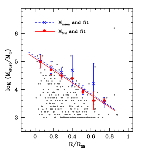
Figure 1: M 33, radial distributions. Left panel: log cluster mass. Grey dots: cluster data; blue crosses and blue short-dashed line: average of 5 most massive clusters in bins $4\farcm 04$ wide (i.e., 1 kpc, $\approx 0.11R_{25}$), and weighted fit; red filled circles and red solid line: median of 5 most massive clusters (i.e., effectively, the third most massive cluster) in the same bins, and fit. Right panel: log surface densities (thick lines) and linear fits (thin lines). Solid: H₂; dotted: HI; dashed: total gas; solid triangles and dotted-long-dashed line: SFR. See text for the fitted relation. The $x$- and $y$- axes of the two panels have the same dynamic ranges, so that the slopes of the fits to the cluster and gas data are directly comparable.

From the weighted fit to the mean, we obtain:

$${\rm log}_{10}\ M_{\rm mean}/M_{\odot}=(-2.2\pm 0.2)R/R_{25}+(5.2\pm 0.1);$$ (1)

the fit to the median yields:

$${\rm log}_{10}\ M_{\rm 3rd}/M_{\odot}=(-2.2\pm 0.2)R/R_{25}+(5.1\pm 0.1).$$ (2)

We note that there is an extremely massive cluster at $\approx 0.85\ R_{25}$, almost at the edge of the available H₂ data and beyond the published radial profiles of $\Sigma_{\rm H2}$ and $\Sigma_{\rm SFR}$. This cluster, the most massive in the galaxy with $M_{\rm clust}\gtrsim 10^{6}M_{\odot}$, sits over one of the brightest spots in the CO J=1-0 map, while there is very little emission detected from the rest of the galaxy at the same galactocentric distance (see Heyer et al., 2004, their Figure 2.). The region is also quite bright at 21 cm, and is the brightest location between 24 and 170 $\mu$m (Heyer et al., 2004; Hippelein et al., 2003; Tabatabaei et al., 2007). Hence, the azimuthally averaged emission of the corresponding annulus would not be representative of the star-forming conditions at the location of the cluster. This cluster has, instead, formed in a local major instability in the interstellar medium.

The SFR and gas surface densities (Heyer et al., 2004), and our linear fits to the data are shown in the right panel of Figure 1. The x-axes of both panels in the figure are the same, whereas the y-axes have the same dynamic ranges, so that the slopes of fits to gas surface densities and cluster masses are directly comparable.

The fits to the available gas are:

$${\rm log}_{10}\ \Sigma_{\rm gas}=(-0.47\pm 0.01)R/R_{25}+(1.363\pm 0.005);$$

$${\rm log}_{10}\ \Sigma_{\rm H_{2}}=(-1.63\pm 0.01)R/R_{25}+(0.84\pm 0.01);$$

$${\rm log}_{10}\ \Sigma_{\rm SFR}=(-2.17\pm 0.02)R/R_{25}+(1.62\pm 0.01);$$

$${\rm log}_{10}\ \Sigma_{\rm H_{I}}=(-0.23\pm 0.02)R/R_{25}+(1.05\pm 0.01).$$

For M 33, then, both the mean and the median of the 5 most massive clusters yield: $M_{\rm mean,3rd}\propto\Sigma_{\rm gas}^{4.7\pm 0.4}$; $M_{\rm mean,3rd}\propto\Sigma_{\rm H_{2}}^{1.3\pm 0.1}$; $M_{\rm mean,3rd}\propto\Sigma_{\rm SFR}^{1.0\pm 0.1}$.

We discard here the possibility that the change in mean and median maximum cluster mass with radius is a statistical effect, due to the number of clusters in each equal sized bin decreasing with increasing radius. If clusters are drawn purely randomly, or stochastically, from the same mass distribution function that declines with mass, and that has a constant upper truncation mass $M_{\rm u}>10^{6}M_{\odot}$, the probability of picking a massive cluster decreases with the size of the sample, i.e., with the number of clusters in the sample. We demonstrate in the following that the change in maximum mass is due to physical causes instead.

Figure 2 shows fits to the median mass clusters in bins, each one containing an equal number of objects from the subsample of 258 clusters with $M_{\rm clust}\geq 10^{3}M_{\odot}$ detected by Sharma et al. (2011) in M 33; the total number of bins increases from 3 (upper left panel) to 6 (lower left panel). The number of clusters in each bin is indicated, and the maximum and median masses are shown, respectively, with black empty triangles and red filled circles.

Two fits to the medians are performed: one including all the bins in each panel (red dashed line), and one omitting the last bin (blue solid line); this bin includes a radial range for which there is no molecular gas data, and always contains the most massive cluster in M 33 (see above), an object whose characteristics do not seem to correlate with the average star-forming conditions at its galactocentric radius. The fits have the form:

$${\rm log_{10}}\ M_{\rm clust}/M_{\odot}=(\beta^{\prime}\pm\sigma_{\beta^{\prime}})R/R_{25}+(\alpha^{\prime}\pm\sigma_{\alpha^{\prime}}),$$ (3)

and their coefficients and their uncertainties are listed, respectively, in the top and bottom of Table 1. When the last bin is included, the slopes $\beta^{\prime}$ of these fits get slowly steeper, as the number of bins increases (see top of Table 1) and the relative importance of the last bin progressively diminishes. If, on the other hand, we exclude the last bin, we find that the slope of the fits to the median cluster mass is $\beta^{\prime}=-2.0\pm 0.3$ (see Table 1, bottom), regardless of the number of bins.

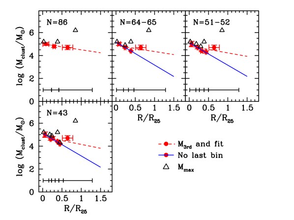
Figure 2: M 33, log cluster mass vs. radius, fits to bins with equal numbers of clusters. The number of bins increases from 3 (upper left panel) to 6 (lower left panel); numbers of clusters in each bin are indicated. The bar at the bottom of each panel shows radial ranges of the bins. Empty triangles: most massive cluster in each bin; filled red circles: median of five most massive clusters (i.e., third most massive cluster) in each bin; red dashed line: fit to medians in all bins; blue solid line: fit to medians excluding last bin. Fits are performed only for three and more bins.

Table 1: Fits to log $M_{\rm 3rd/M_{\odot}}$ vs. $R/R_{25}$, Figure 2 and eq. 3

$N_{b}$	$N_{\rm cl}$	$\beta^{\prime}\pm\sigma_{\beta^{\prime}}$	$\alpha^{\prime}\pm\sigma_{\alpha^{\prime}}$	RMS
3	86	$(-0.5\pm 0.2)$	$(5.01\pm 0.08)$	0.04
4	64-65	$(-0.5\pm 0.6)$	$(4.9\pm 0.2)$	0.2
5	51-52	$(-0.6\pm 0.6)$	$(4.8\pm 0.2)$	0.2
6	43	$(-0.7\pm 0.6)$	$(4.8\pm 0.2)$	0.2
Without last bin
3	64-65	$(-2.00\pm 0.02)$	$(5.17\pm 0.01)$	0.003
4	51-52	$(-2.0\pm 0.3)$	$(5.1\pm 0.1)$	0.05
5	43	$(-2.0\pm 0.3)$	$(5.1\pm 0.1)$	0.1

Note. — Col. (1): number of bins. Col. (2): number of clusters in each bin. Col. (3): best-fit slope. Col. (4): best-fit intercept. Col. (5): best-fit RMS residual.

If, instead of the median, we consider the 90^th percentile cluster (i.e., the 9^th, 6^th, 5^th, and 4^th most massive cluster, respectively, for 3, 4, 5, and 6 bins), the correlation (including the last bin) is consistent in all cases with ${\rm log_{10}}\ M_{\rm 90th}/M_{\odot}=1.2\pm 0.2R/R_{25}+(4.7\pm 0.1)$. Thus, the relation between cluster mass and radius is slightly shallower than for $M_{\rm 3rd}$, but still quite robust and definitely not flat. We note here, though, that for large samples (for example, of a few hundred clusters) the mass of the 90^th percentile point might already be one or two orders of magnitude below that of the most massive clusters, and hence would not be a good estimator for this particular problem.

In order to convince the reader that the intrinsic mass distribution of clusters changes as a function of radius, we perform a Kolmogorov-Smirnov (K-S) test on the 6 different radial subsamples presented in the bottom left panel of Figure 2. Figure 3 shows the cumulative probability distributions and median radii of each subsample, and the $D$ and $P$ values for every bin pair are given in Table 2 (higher bin number indicates larger radius). The visual impression, that the inner bins are different from the outer ones, is confirmed by the K-S statistic: assuming that sample pairs with $P<0.05$ are taken from different distribution functions with high significance, we conclude that bins 1 and 2, within $R=0.22\ R_{25}$, are different from bins 5 and 6, beyond $R=0.42\ R_{25}$. Bin 3 also differs from bin 6, such that the change of the cluster mass distribution function appears to be gradual, rather than stepwise.

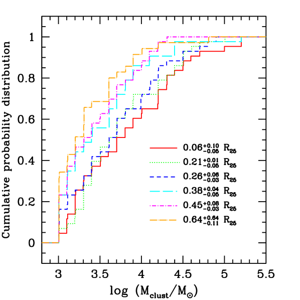
Figure 3: K-S test; cumulative probability distributions of mass for clusters with $M_{\rm clust}\geq 10^{3}\ M_{\odot}$ in the six annuli whose median radii are indicated. Red solid line: bin 1, $R=0.06^{+0.10}_{-0.05}\ R_{25}$; green dotted line: bin 2, $R=0.21^{+0.01}_{-0.05}\ R_{25}$; blue short dashed line: bin 3, $R=0.26^{+0.06}_{-0.03}\ R_{25}$; cyan long dashed line: bin 4, $R=0.38^{+0.04}_{-0.05}\ R_{25}$; purple short dashed-dotted line: bin 5, $R=0.45^{+0.08}_{-0.03}\ R_{25}$; orange long dashed-dotted line: bin 6, $R=0.64^{+0.64}_{-0.11}\ R_{25}$.

Table 2
K-S test $D$ and $P$ values
            $D$ $P$ $D$ $P$ $D$ $P$ $D$ $P$ $D$ $P$ Bin 2 3 4 5 6 1 0.56 0.9168 0.78 0.5799 1.22 0.1005 1.45 0.0307 1.63 0.0096 2 0.67 0.7651 1.33 0.0569 1.45 0.0307 1.72 0.0052 3 1.00 0.2694 1.11 0.1687 1.63 0.0096 4 0.56 0.9168 1.10 0.1797 5 0.69 0.7271

These results rule out the size of sample effect, according to which no correlation ($\beta^{\prime}=0$) is expected between maximum cluster mass and galactic radius. From the ratio $\sigma_{\beta^{\prime}}/\beta^{\prime}$, it follows that the falsification of stochastic sampling is at a confidence level of at least 7$\sigma$.

5 Conclusions

We have analyzed the relationship between maximum cluster mass and gas surface density in M 33, in order to explore the suggestion that maximum cluster mass is determined by physical processes, e.g., the equilibrium pressure between cluster forming cores and the ambient interstellar medium (Larsen, 2002; Billett et al., 2002), and since the existence of such a relationship can reconcile, via the IGIMF theory, SFR measurements derived, respectively, from H$\alpha$ and FUV emission in galaxy disks.

To this end, we have used published gas data of M 33 (Corbelli, 2003; Heyer et al., 2004), and a catalog of more than 600 young star clusters in its disk, also from the literature (Sharma et al., 2011). Because often the most massive cluster in a range of galactocentric distances is formed under conditions that are not average for the annulus, we find that it is best, in the present annular averaging approach, to use the median of the five most massive clusters (i.e, the third most massive cluster) in each bin for this kind of analysis.

We have compared radial distributions, and have found that $M_{\rm 3rd}\propto\Sigma_{\rm H_{2}}^{1.3\pm 0.1}$, while $M_{\rm 3rd}\propto\Sigma_{\rm SFR}^{1.0\pm 0.1}$ (in a range consistent with the expectations from pressure equilibrium considerations). On the other hand, $M_{\rm max}\propto\Sigma_{\rm gas}^{4.7\pm 0.4}$, steeper than needed to explain the H$\alpha$ cut-off in galaxy disks. Both this correlation and the steeper than average star formation law might be related to the shallowness of the HI profile.

In order to test whether the trend of $M_{\rm max}$ (or its proxy, $M_{\rm 3rd}$), with galactocentric radius is consistent with random sampling from the cluster mass function, we have also measured the radial distribution of maximum mass in 3 to 6 bins with an equal number of clusters in each bin. After accounting for the presence of the most massive cluster in the galaxy at $\approx 0.85R_{25}$, whose formation environment is certainly not represented by the average conditions across the galaxy at its galactocentric distance, and for the lack of gas data beyond this same radius, we find exactly the same results as before, regardless of the width of the bins. A K-S test on the mass distributions in these bins suggests that the two bins closest to the galaxy center are different from the two most external ones, i.e., that the mass distribution function changes with radius.

The significant decrease of ${\rm log}\ M_{\rm max}$ with radial distance in M 33, as a power law with index $\beta^{\prime}\approx-2.0\pm 0.3$, and despite there being the same number of clusters per radial bin, rules out random sampling with extremely high confidence. This one galaxy, thus, falsifies the hypothesis that the most massive cluster masses scale with the size of the sample. Instead, the range of star cluster masses is driven by environmental physics. Indeed, the available data for M 33 suggest log${}_{10}\ M_{\rm 3rd}\propto\ {\rm log}_{10}\Sigma_{\rm H_{2}}\propto\ {\rm log}_{10}\Sigma_{\rm SFR}$. This, however, may be merely a (trivial) self-consistent result because, after all, stars may form from molecular clouds in a free-fall timescale and subsequently destroy the clouds (Hartmann et al., 2001). The non-trivial challenge remains to answer how the interstellar medium, and thus mostly the HI gas, arranges itself to form molecular clouds.

References

- Bell & Kennicutt (2001) Bell, E. F., & Kennicutt, R. C., Jr. 2001, ApJ, 548, 681
- Billett et al. (2002) Billett, O. H., Hunter, D. A., & Elmegreen, B. G. 2002, AJ, 123, 1454
- Boissier et al. (2007) Boissier, S., Gil de Paz, A., Boselli, A., et al. 2007, ApJS, 173, 524
- Boselli et al. (2009) Boselli, A., Boissier, S., Cortese, L., et al. 2009, ApJ, 706, 1527
- Corbelli (2003) Corbelli, E. 2003, MNRAS, 342, 199
- Corbelli & Schneider (1997) Corbelli, E., & Schneider, S. E. 1997, ApJ, 479, 244
- Demleitner et al. (2001) Demleitner, M., Accomazzi, A., Eichhorn, G., et al. 2001, Astronomical Data Analysis Software and Systems X, 238, 321
- Elmegreen (1983) Elmegreen, B. G. 1983, MNRAS, 2003, 1011
- Freedman et al. (1991) Freedman, W. L., Wilson, C. D., & Madore, B. F. 1991, ApJ, 372, 455
- Gil de Paz et al. (2007) Gil de Paz, A., Boissier, S., Madore, B. F., et al. 2007, ApJS, 173, 185
- Greenawalt et al. (1998) Greenawalt, B., Walterbos, R. A. M., Thilker, D., & Hoopes, C. G. 1998, ApJ, 506, 135
- Hartmann et al. (2001) Hartmann, L., Ballesteros-Paredes, J., & Bergin, E. A. 2001, ApJ, 562, 852
- Heyer et al. (2004) Heyer, M. H., Corbelli, E., Schneider, S. E., & Young, J. S. 2004, ApJ, 602, 723
- Hippelein et al. (2003) Hippelein, H., Haas, M., Tuffs, R. J., et al. 2003, A&A, 407, 137
- Hoopes & Walterbos (2000) Hoopes, C. G., & Walterbos, R. A. M. 2000, ApJ, 541, 597
- Kennicutt (1998) Kennicutt, R. C., Jr. 1998, ARA&A, 36, 189
- Kroupa & Weidner (2003) Kroupa, P., & Weidner, C. 2003, ApJ,598, 1076
- Larsen (2002) Larsen, S. S. 2002, AJ, 124, 1393
- Lada & Lada (2003) Lada, C. J., & Lada, E. A. 2003, ARA&A, 41, 57
- Lee et al. (2009) Lee, J. C., Gil de Paz, A., Tremonti, C., et al. 2009, ApJ, 706, 599
- Leitherer et al. (1999) Leitherer, C., Schaerer, D., Goldader, J. D., et al. 1999, ApJS, 123, 3
- Marks & Kroupa (2012) Marks, M., & Kroupa, P. 2012, arXiv:1205.1508
- Maschberger & Kroupa (2007) Maschberger, T., & Kroupa, P. 2007, MNRAS, 379, 34
- McConnachie et al. (2010) McConnachie, A. W., Ferguson, A. M. N., Irwin, M. J., et al. 2010, ApJ, 723, 1038
- Meurer et al. (2009) Meurer, G. R., Wong, O. I., Kim, J. H., et al. 2009, ApJ, 695, 765