Electron optical depths and temperatures of symbiotic nebulae from Thomson scattering

Abstract

Symbiotic binaries are comprised of nebulae, whose densest portions have electron concentrations of $10^{8}-10^{12}$ cm^-3 and extend to a few AU. They are optically thick enough to cause a measurable effect of the scattering of photons on free electrons. In this paper we introduce modelling the extended wings of strong emission lines by the electron scattering with the aim to determine the electron optical depth, $\tau_{\rm e}$, and temperature, $T_{\rm e}$, of symbiotic nebulae. We applied our profile-fitting analysis to the broad wings of the OVI 1032, 1038 Å doublet and HeII 1640 Å emission line, measured in the spectra of symbiotic stars AG Dra, Z And and V1016 Cyg. Synthetic profiles fit well the observed wings. By this way we determined $\tau_{\rm e}$ and $T_{\rm e}$ of the layer of electrons, throughout which the line photons are transferred. During quiescent phases, the mean $\tau_{\rm e}=0.056\pm 0.006$ and $T_{\rm e}=19\,200\pm 2\,300$ K, while during active phases, mean quantities of both parameters increased to $\tau_{\rm e}=0.64\pm 0.11$ and $T_{\rm e}=32\,300\pm 2\,000$ K. During quiescent phases, the faint electron-scattering wings are caused mainly by free electrons from/around the accretion disk and the ionized wind from the hot star with the total column density, $N_{\rm e}\la 10^{23}$  cm^-2. During active phases, the large values of $\tau_{\rm e}$ are caused by a supplement of free electrons into the binary environment as a result of the enhanced wind from the hot star, which increases $N_{\rm e}$ to $\sim 10^{24}$  cm^-2.

1 Introduction

Symbiotic stars are long-period interacting binaries with orbital periods in the range of years. In their spectra we can recognize three main sources of radiation. The first one is represented by a giant star of spectral type (G-)K-M, the second one is a very hot ($T_{\rm h}\ga 10^{5}\,\rm K$) compact star, which is in most cases a white dwarf accreting from the wind of the giant. The third component of radiation is produced by a nebula, which represents the ionized fraction of the circumstellar material in the binary (e.g. Boyarchuk, 1967; Seaquist, Taylor & Button, 1984, hereafter STB; Kenyon, 1986; Nussbaumer & Vogel, 1987; Corradi et al., 2003; Skopal, 2005, and references therein). As a result, the circumstellar environment of symbiotic binaries comprises energetic photons from the hot star with luminosities of $10^{2}-10^{4}$  $L_{\sun}$ (e.g. Mürset et al., 1991; Greiner et al., 1997; Skopal, 2005), neutral particles produced by the cool giant at rates of a few times $10^{-7}$  $M_{\sun}\,{\rm yr}^{-1}$ (e.g. STB, Mikolajewska et al., 2002; Skopal, 2005), and ions and free electrons resulting from the processes of ionization. Symbiotic stars thus represent ideal objects for studying effects of Rayleigh, Raman and Thomson scattering. Raman and Rayleigh scattering results from interaction between the hot star photons and the neutral atoms in the giant’s wind. They are important tools in mapping the ionization structure of symbiotic binaries (e.g. Isliker et al., 1989; Nussbaumer et al., 1989; Schmid, 1998; Birriel, 2004; Lee, 2009, 2012). In contrast, the Thomson scattering of photons by free electrons acts within the ionized part of the symbiotic stars environment, and thus can diagnose the symbiotic nebula. In the spectrum, we can indicate this effect in the form of shallow, wide wings of the strongest emission lines, which photons are scattered by free electrons, and thus are Doppler shifted by their thermal motion to both the red and blue side of the line. The effect of this process is weak and wavelength independent, because of a very small and constant value of the Thomson cross-section, $\sigma_{\rm T}=6.652\times 10^{-25}$ cm². Nevertheless, the densest portions of symbiotic nebulae with electron concentrations of $\log(n_{\rm e})\sim 8-12$ ($n_{\rm e}$ in  cm^-3), could be optically thick enough to cause a measurable effect of the electron scattering. From this point of view, strong emission lines of highly ionized elements that are formed in the densest part of the ionized medium in a vicinity of the hot white dwarf, represent the best candidates.

Originally, Schmid et al. (1999) suggested that the broad wings of the OVI 1032 and 1038 Å resonance lines could be explained by scattering of the OVI photons by free electrons. Young et al. (2005) successfully compared a model of the electron scattering wings with the OVI doublet in the AG Dra spectrum. This process was also used by Jung & Lee (2004) to model the broad H$\alpha$ wings in the spectrum of the symbiotic star V1016 Cyg as an alternative to the Raman scattering of Ly$\beta$ photons on atomic hydrogen. Skopal et al. (2009) used the electron scattering of the OVI 1032, 1038 Å doublet and HeII 1640 Å line in the AG Dra spectrum to support the origin of the X-ray–UV flux anticorrelation, revealed by modelling the SED.

In this paper we describe a simplified method for fitting the broad wings of intense emission lines by the electron scattering process (Sect. 3). We applied our profile-fitting procedure to the OVI resonance doublet and the HeII 1640 Å line, observed in the spectra of symbiotic stars AG Dra, Z And and V1016 Cyg, with the aim to determine the electron optical depth, $\tau_{\rm e}$, and temperature, $T_{\rm e}$, of their nebulae. Sect. 4 presents the results and their discussion. Conclusions are found in Sects. 5.

2 Observations and data treatment

For the purpose of this paper, we used extremely intense emission lines of the OVI 1032, 1038 Å doublet observed in the FUSE (Far Ultraviolet Spectroscopic Explorer), BEFS (Berkeley Extreme and Far-UV Spectrometer) and TUES (Tübingen Ultraviolet Echelle Spectrograph) spectra of AG Dra, Z And and V1016 Cyg. We used also the strong emission line HeII 1640 Å in the high-resolution IUE (International Ultraviolet Explorer) spectra of AG Dra. The spectra were obtained from the satellite archives with the aid of the Multimission Archive at the Space Telescope Science Institute (MAST). They are summarized in Table 1.

The FUSE spectra were processed by the calibration pipeline version 3.0.7, 3.0.8 and 2.4.1. We used the calibrated time-tag observations (TTAG photon collecting mode). Before adding the flux from all exposures we applied an appropriate wavelength shift relative to one so to get the best overlapping of the absorption features. Then we co-added spectra of individual exposures and weighted them according to their exposure times. The wavelength scale of the spectra was calibrated with the aid of the interstellar absorption lines (e.g. Rogerson & Ewell, 1984). Accuracy of such calibration is of $\pm$ 0.05 Å. Finally, we binned the resulting spectrum within 0.025 Å.

Table 1: Log of spectroscopic observations.

Date	Julian date	Orb.	Obs.	Line${}^{b})$
(dd/mm/yyyy)	- 2 400 000	phase${}^{a})$	Satellite
AG Dra
11/12/1981	44949.5	0.38	IUE	HeII
18/09/1993	49248.5	0.22	BEFS	OVI
29/06/1994	49532.5	0.74	IUE	HeII
09/07/1994	49542.5	0.75	IUE	HeII
12/07/1994	49545.5	0.76	IUE	HeII
28/07/1994	49561.5	0.79	IUE	HeII
17/09/1994	49612.5	0.88	IUE	HeII
28/07/1995	49927.5	0.46	IUE	HeII
14/02/1996	50127.5	0.82	IUE	HeII
22/11/1996	50409.5	0.33	TUES	OVI
16/03/2000	51619.5	0.54	FUSE	OVI
25/04/2001	52024.5	0.28	FUSE	OVI
14/11/2003	52957.5	0.98	FUSE	OVI
24/06/2004	53180.5	0.38	FUSE	OVI
25/12/2004	53364.5	0.72	FUSE	OVI
15/03/2007	54174.5	0.20	FUSE	OVI
Z And
05/07/2002	52460.5	0.90	FUSE	OVI
04/08/2003	52855.5	0.42	FUSE	OVI
V1016 Cyg
10/08/2000	51766.5	?	FUSE	OVI

${}^{a})$ - According to Fekel et al. (2000), ${}^{b})$ - HeII 1640 Å, OVI 1032, 1038 Å doublet,

All the spectra were corrected for heliocentric velocity including that of the satellite, and dereddened with $E_{\rm B-V}$ = 0.30 (Z And, Mürset et al., 1991), 0.28 (V1016 Cyg, Nussbaumer & Schild, 1981) and 0.08 for AG Dra (Birriel et al., 2000), using the extinction curve of Cardelli et al. (1989).

3 The model

3.1 Assumptions and simplifications

Thomson scattering represents a special case of the scattering of a photon off a free electron, which is fully elastic (i.e. the photon energy does not change). In the real case, the photon always transfers some of its energy to the electron, which shifts its wavelength by $\sim$+0.024 Å, the so-called Compton wavelength of the electron. However, the Doppler effect arising from the thermal motion of free electrons leads to significantly larger shifts to both sides of the spectrum. Therefore, the elastic Thomson scattering is a good approximation in studying scattering of low-energy photons ($h\nu<<m_{\rm e}c^{2}$) off non-relativistic electrons (see e.g. Rosswog & Brüggen, 2007, in detail).

To model the effect of the electron scattering we have to know how the scattered photons are redistributed in frequencies and directions. It was shown by Hummer & Mihalas (1967) that it is convenient and sufficiently accurate to regard the radiation field, from which scattering occurs, as isotropic, so that the direction can be averaged out. Therefore, for the sake of simplicity, we consider isotropic scattering with Maxwellian distribution of electron velocities. Under these assumptions the redistribution function can be expressed in a form (Mihalas, 1970),

$$R_{\rm e}\left(\nu,\nu^{{}^{\prime}}\right)=\frac{1}{w}\left(\frac{e^{-{\left|\frac{\nu-\nu^{{}^{\prime}}}{2w}\right|}^{2}}}{\sqrt{\pi}}\right)-\left|\frac{\nu-\nu^{{}^{\prime}}}{2w}\right|{\rm erfc}\left|\frac{\nu-\nu^{{}^{\prime}}}{2w}\right|,$$ (1)

where $\nu$ and $\nu^{{}^{\prime}}$ are frequencies of radiation before and after the scattering and $w$ is the electron Doppler width,

$$w=\frac{\nu_{0}}{c}\sqrt{\frac{2kT_{\rm e}}{m_{\rm e}}},$$ (2)

and the complementary error function $\rm{erfc(x)}$ is defined as

$${\rm erfc}\left(x\right)=\frac{2}{\sqrt{\pi}}\int^{\infty}_{x}e^{-z^{2}}dz.$$ (3)

To calculate the electron-scattering wings profiles, we adopted a simplified scheme of Münch (1950), which assumes that a plane-parallel layer of free electrons of the optical thickness $\tau_{\rm e}$ and the temperature $T_{\rm e}$ is irradiated by the line photons, and that the electrons are segregated from the other opacity sources, which implies no change in the equivalent width of the line. In our case, this assumption corresponds to modelling the wings of highly ionized OVI and HeII lines, which are formed within the O⁺⁵ and/or He⁺ zone close to the hot white dwarf photosphere, and the layer of free electrons, where the Thomson scattering arises, is located above the line formation region.

According to the radiative transfer equation, assuming that the electron scattering is the only process attenuating the original line photons, the observed line flux can be expressed as

$$F^{\rm obs}=F_{0}\,e^{-\tau_{\rm e}},$$ (4)

where $F_{0}$ is the line flux before scattering, $\tau_{\rm e}=\sigma_{\rm T}N_{\rm e}$ is the electron optical depth and $N_{\rm e}$ is the column density of free electrons along the line of sight. As the scattered fraction of the original flux is redistributed into the line wings so that the equivalent width before and after the scattering is constant, $F_{\rm wing}=F_{0}-F^{\rm obs}=F_{0}(1-e^{-\tau_{\rm e}})$. Then the line profile after it emerges from the layer of scattering electrons may be approximated by (see also Castor et al., 1970)

$$\Psi(x)=e^{-\tau_{\rm e}}\Phi(x)+(1-e^{-\tau_{\rm e}})\!\int\limits_{\infty}^{-\infty}\!\Phi(x^{{}^{\prime}})R_{e}(x^{{}^{\prime}},x){\rm d}x^{{}^{\prime}},$$ (5)

where $\Phi(x)$ is the incident line profile, $R_{\rm e}(x^{{}^{\prime}},x)$ is the redistribution function for Thomson scattering (Eq. (1)) and $x$ or $x^{{}^{\prime}}$ is a frequency displacement from the line center in units of electron Doppler width before and after the scattering, respectively. So, the first right-side term of Eq. (5) represents the original flux at $x$ attenuated by the scattering (Eq. (4)), and its scattered, $(1-e^{-\tau_{\rm e}})$, fraction is redistributed in the wings (the second term). Note that the scattered profile used previously by e.g. Castor et al. (1970) represents a special case of Eq. (5) for $\tau_{\rm e}\ll 1$.

To fit the theoretical profile (5) to observations, means to determine its variables, $\tau_{\rm e}$, $T_{\rm e}$, and those of the incident profile $\Phi(x)$.

Figure 1: Examples of the observed (solid lines) and the incident (dotted lines) profiles of the OVI 1032 Å line. Arrows denote the red-side emission bumps.

3.2 The incident profile

First, we estimated the continuum level from a large wavelength interval around the OVI lines by a linear fit to the noise in the spectrum. In the case of the HeII 1640 Å line, the continuum level was estimated with the aid of the corresponding low-resolution spectrum. Second, we approximated the incident profile $\Phi(\lambda)$ in the model (5) as follows. The HeII 1640 Å line was possible to fit with a single Gauss curve. The fit of the observed emission core provided the first estimate of its position, width and the height. The OVI 1032 Å line is in most cases asymmetric with respect to its reference wavelength. Its blue emission wing is steeper than the red one, being cut by an absorption component (see Fig. 1). It is probably caused by the scattering in the line at the close vicinity of the white dwarf within the densest part of the wind moving to the observer. This absorption can be more pronounced during active phases, when a higher mass-loss rate is observed (Skopal, 2006). The observation of AG Dra from 2007 May 15, made during the 2006-08 active phase, is consistent with this view (see the left panel of Fig. 1). The scattering in the line operates within the line formation region. Therefore, we take the incident profile of the OVI 1032 Å line as a sum of emission and absorption Gaussians. The incident emission of the OVI 1038 Å line was not possible to reconstruct by a direct fitting of its observed remainder, because of a strong influence by the absorption of the interstellar molecular hydrogen, $H_{2}$ (e.g. Schmid et al., 1999). Therefore, we reconstructed the incident OVI 1038 Å profile with the aid of the theoretical ratio of the doublet lines with the assumption that they have the same width (see below).

Based on the above mentioned observational properties of the OVI 1032, 1038 Å doublet, we reconstructed its incident profile by a superposition of three Gaussians,

$$\Phi(\lambda)=\sum_{\rm n=1}^{\rm 3}I_{\rm n}\exp\left[{-\frac{1}{2}\left(\frac{\lambda-\lambda_{\rm n}}{\sigma_{\rm n}}\right)^{2}}\right],$$ (6)

where indices n = 1 and 3 denote the Gaussians of the emission cores at $\lambda_{1}\sim 1032$ Å and $\lambda_{3}\sim 1038$ Å. The second curve (n = 2) represents the absorption component, which cut the blue side of the 1032 Å emission line (Fig. 1). However, this rather strong absorption did not reproduce the narrow one seen in the scale of Figs. 2 and 3 as a P-Cyg component in the 1032 Å line, but not recognizable in the scale of Fig. 1. Only for the V1016 Cyg spectrum, due to a symmetrical emission core of the 1032 Åline, it was possible to fit this narrow P-Cyg absorption by the $\rm{\scriptsize I}_{2}$ component (see the right panel of Fig. 3). Irrespectively of its origin, we neglected its influece to the profile.

The effect of the interstellar $H_{2}$ absorption to the OVI 1038 Å line profile was significant in the spectra of Z And and V1016 Cyg, because of a large amount of interstellar matter on the line of sight to these objects ($E_{\rm B-V}\sim 0.3$). As a result, the observed intensity ratio $\rm{\scriptsize I}_{1}/\rm{\scriptsize I}_{3}$ was $\approx 7$ for Z And and $\approx 15$ for V1016 Cyg. Therefore, we reconstructed the original OVI 1038 Å line adopting the theoretical ratio $\rm{\scriptsize I}_{1}/\rm{\scriptsize I}_{3}=2$, $\sigma_{3}=\sigma_{1}$ and $\lambda_{3}$ so to fit the emission remainder of the line. The absorption effect from the $H_{2}$ molecules was apparently fainter on the AG Dra spectra ($E_{\rm B-V}\sim 0.08$, $\rm{\scriptsize I}_{1}/\rm{\scriptsize I}_{3}\approx 2$), and thus the estimate of the initial OVI 1038 Å line profile was more trustworthy.

Some spectra show a noticeable additional emission features at the red side of the 1032 Å and 1038 Å line cores up to $\sim 10$% of their height. We did not investigate the origin of these features and did not take them into account in the fitting procedure. However, in the AG Dra spectrum from 2007 March, the unknown emission features were rather strong. Therefore, we included them to the incident OVI 1032 Å, 1038 Å line profiles as an additional Gaussians (see Fig. 1).

3.3 Profile-fitting analysis

First, we selected the flux-points of the observed profile(s), $F^{\rm obs}(\lambda_{\rm i})$, for fitting with the function (5). They were selected from the observed profiles by omitting some artificial (sharp) emission/absorption features and the depression around the Ly${\beta}$ line, caused by the Rayleigh scattering (see Fig. 2). To find the best solution, we calculated a grid of models for reasonable ranges of the fitting parameters, $I_{\rm n}$, $\sigma_{\rm n}$, $\lambda_{\rm n}$ for the original profile $\Phi(x)$ and $\tau_{\rm e}$, $T_{\rm e}$ for the scattered wings. In the case of the OVI 1032 Å, 1038 Å doublet, the parameters $I_{3}$, $\sigma_{3}$, $\lambda_{3}$ of its 1038 Å component were estimated according to the properties of both the doublet lines, as described in Sect. 3.2. The grid of models was prepared with steps $\Delta\tau_{\rm e}=0.0005$, $\Delta T_{\rm e}=100$ K, $\Delta I_{\rm n}=I_{\rm n}/100$, $\Delta\sigma_{\rm n}=0.001$ and $\Delta\lambda_{\rm n}=0.001$ Å. Finally, we selected the model corresponding to a minimum of the function

$$\chi^{2}_{\rm red}=\frac{1}{\aleph}\sum_{\rm i=1}^{\rm N}\left[\frac{F^{\rm obs}(\lambda_{\rm i})-\Psi(\lambda_{\rm i})}{\Delta F^{\rm obs}(\lambda_{\rm i})}\right]^{2},$$ (7)

where $F^{\rm obs}(\lambda_{\rm i})$ are the observed fluxes of the profile, $N$ is their number ($\approx 200$), $\aleph$ is the number of d.o.f., $\Delta F^{\rm obs}(\lambda_{\rm i})$ are their errors and $\Psi(\lambda_{\rm i})$ are theoretical fluxes.

Errors in the selected flux points were around of 10–15% of the line wings. Based on them we determined uncertainties in $T_{\rm e}$ and $\tau_{\rm e}$ for individual spectra. To obtain a rough estimate of the corresponding range of $T_{\rm e}$ we fixed other fitting parameters and varied $T_{\rm e}$ so to fit fluxes $F^{\rm obs}(\lambda_{\rm i})\pm\Delta F^{\rm obs}(\lambda_{\rm i})$. Similarly we proceeded to estimate the limits for $\tau_{\rm e}$. Such the estimated ranges of fitting parameters can be as large as $\sim 50$% of the best model value and are asymmetrically placed with respect to it (see Table 2). This is a result of the non-uniformly distributed fluxes determining the profile of electron-scattered wings (see the beginning of Sect. 3.3.). In the case of the AG Dra spectrum from 14/02/1996, the relatively small uncertainties in $T_{\rm e}$ and $\tau_{\rm e}$, but the large value of $\chi^{2}_{\rm red}$ probably reflect underestimated flux errors, $\Delta F^{\rm obs}(\lambda_{\rm i})$. Large flux uncertainties on the spectrum from 22/11/1996 and poorly defined continuum level did not allow us to estimate the upper limit of $T_{\rm e}$ (see Fig. 2).

4 Results and Discussion

The resulting fits are shown in Fig. 2 and 3 and corresponding parameters are in Table 2. Significant changes in $\tau_{\rm e}$ and $T_{\rm e}$ reflect different properties of the symbiotic nebula during different levels of the activity. During quiescent phases, the mean $T_{\rm e}=19\,200\pm 2\,300$ K, $\tau_{\rm e}=0.056\pm 0.006$, while during active phases $T_{\rm e}=32\,300\pm 2\,000$ K, $\tau_{\rm e}=0.64\pm 0.11$, respectively. Here the uncertainties represent rms errors of the average values.

The average quantities of $T_{\rm e}$ and $\tau_{\rm e}$ as derived from quiescent and active phases agree well with those found independently by modelling the SED (e.g. Skopal, 2005; Skopal et al., 2009). More than one order of magnitude difference in $\tau_{\rm e}$ (i.e. in $N_{\rm e}$) reflect a significant increase of free electrons on the line of sight in the direction to the hot star during active phases. The origin of this change is shortly discussed in Sects. 4.2. and 4.3.

4.1 Application to selected symbiotic stars

4.1.1 AG Dra

AG Dra is a yellow symbiotic star comprising a cool giant of a K2 III spectral type (Mürset & Schmid, 1999). It is located at a high galactic latitude of $41^{\circ}$, which implies that its spectrum is less affected by the interstellar matter. As a result, the line ratio $I$(1038 Å)/$I$(1032 Å) was close to its theoretical value of 0.5, which made the modelling of the OVI doublet more trustworthy (Sect. 3.2).

By modelling the UV/IR continuum of AG Dra, Skopal (2005) found that the mean electron temperature of the nebula during quiescent phase and/or small bursts runs between 18 000 and 21 800 K, while during major outbursts (1980-81, 1994-5, 2006-7, Fig. 2), the nebula significantly strengthens and increases its mean $T_{\rm e}$ to $\sim 35\,000$ K. In this work we confirmed these results independently by the profile-fitting analysis of the electron scattered wings. We found that during a quiescent phase, the mean $T_{\rm e}=21\,700\pm 3\,600$ K, while during active phases $T_{\rm e}=32\,300\pm 2\,000$ K. Also $\tau_{\rm e}$ is a function of the star’s activity. Our analysis revealed $\tau_{\rm e}=0.063\pm 0.007$ and $0.64\pm 0.11$ during quiescence and activity, respectively (Table 2, Fig. 2 and 3).

In the 15/03/2007 spectrum, a relatively high value of $\tau_{\rm e}=0.20$, but very faint wings of the OVI doublet (see Fig. 2) is caused by the weak incident line flux, $F_{0}$, because $F_{\rm wing}/F_{0}=1-e^{-\tau_{\rm e}}$ (Sect. 3.1., Fig. 1). So, the well detectable electron scattering wings reflect a relatively large amount of free electrons on the line of sight during the transition from the major 2006 outburst.

Figure 2: Top panel shows the $U$ light curve of AG Dra from 1977. Active phases are characterized by outbursts with multiple maxima. The data are from Skopal et al. (2012). Bottom panels compare the observed (dotted + enhanced line) and modelled (solid smooth line) broad wings of the OVI 1032, 1038 Å doublet and the HeII 1640 Å line at different stages of activity. The enhanced parts of the observed profile were fitted with the function (5). Horizontal dotted line represents the level of the continuum. Timing of individual observations are given in Table 1 (arrows in the top panel). Fluxes are in units of 10^-12$\,\rm\,erg\,cm^{-2}\,s^{-1}\,\AA^{-1}$.

Figure 3: As in Fig. 2, but for Z And and V1016 Cyg.

4.1.2 Z And

Z And is considered to be a prototype of symbiotic stars. Here the white dwarf accretes from the stellar wind of a M3-4 III red giant (e.g. Fernandéz-Castro et al., 1988). During active phases, the light curve shows 2–3 mag brightenings, while the quiescent phase is characterized by a wave-like orbitally-related variation (e.g. Belyakina, 1985; Formiggini & Leibowitz, 1994; Skopal et al., 2006).

Two FUSE spectra used in this work were observed at the end of the major 2000-03 outbursts, 05/07/2002, and just after the optical rebrightening on 04/08/2003 (see Fig. 1 of Skopal et al., 2006). The electron scattering wings observed during both dates (Fig. 3) corresponded to very similar quantities of the fitting parameters, $T_{\rm e}\sim 16\,500$ K, $\tau_{\rm e}\sim 0.050$ and $T_{\rm e}\sim 15\,300$ K, $\tau_{\rm e}\sim 0.051$, respectively (Table 2). Electron temperatures are consistent with those derived from modelling the SED in the continuum (Skopal, 2005).

Table 2: Best solutions of Eq. (7) for $\tau_{\rm e}$ and $T_{\rm e}$ and their ranges $\Delta\tau_{\rm e}$ and $\Delta T_{\rm e}$, corresponding to $\Delta F^{\rm obs}(\lambda_{\rm i})$ (see Sect. 3.3).

Date	Stage⋆	$\tau_{\rm e}$	$\Delta\tau_{\rm e}$	$T_{\rm e}$	$\Delta T_{\rm e}$	$\chi^{2}_{\rm red}$
(dd/mm/yyyy)				[K]	[K]
AG Dra
11/12/1981	A	0.39	0.26–0.55	40 100	22 500–47 200	0.6
18/09/1993	T	0.18	0.15–0.21	20 200	14 600–23 100	1.9
29/06/1994	A	0.39	0.34–0.44	32 700	29 700–34 900	1.6
09/07/1994	A	1.17	1.0–1.4	31 000	28 800–34 500	3.6
12/07/1994	A	0.86	0.70–1.1	29 100	25 300–38 700	3.0
28/07/1994	A	0.80	0.69–0.95	41 300	40 100–46 700	2.5
17/09/1994	A	0.49	0.36–0.66	25 400	14 900–27 400	1.2
28/07/1995	A	0.39	0.33–0.46	28 800	27 500–33 500	0.9
14/02/1996	T	0.30	0.26–0.35	14 300	13 700–15 800	12.1
22/11/1996	T	0.23	0.13–0.34	23 900	18 600-$>$90 000	11.6
16/03/2000	Q	0.044	0.033–0.056	12 800	7 600–18 500	1.0
25/04/2001	Q	0.065	0.051–0.078	23 100	22 900–25 200	1.9
14/11/2003	T	0.084	0.073–0.096	29 900	16 200–41 900	1.2
24/06/2004	Q	0.063	0.051–0.074	20 300	11 200–24 000	0.8
25/12/2004	Q	0.078	0.066–0.091	30 700	29 100–38 900	1.8
15/03/2007	T	0.20	0.16–0.25	21 300	9 600–27 900	2.3
Z And
05/07/2002	Q	0.050	0.042–0.058	16 500	8 600–22 300	2.3
04/08/2003	Q	0.051	0.045–0.056	15 300	10 300–22 400	1.5
V1016 Cyg
10/08/2000	Q	0.038	0.031–0.044	16 000	8 200–26 100	2.0

^⋆ A – active phase, Q – quiescent phase, T – transition to quiescence

4.1.3 V1016 Cyg

V1016 Cyg is a member of a small group of symbiotic stars called symbiotic novae. In 1964 it underwent a nova-like outburst (McCuskey, 1965), during which the star’s brightness increased from m${}_{\rm pg}\sim 15.5$ to $\sim 10.5$ mag in 1971, following a gradual small decrease to $\sim 11.7$ in 2000 (see Fig. 1 of Parimucha et al., 2002).

There was only one well exposed spectrum in the FUSE archive, from 10/08/2000. The wings of the OVI doublet are clearly visible, although the contamination of the 1038Å line is significant ($E_{\rm B-V}=0.28$ mag). In this spectrum we were able to fit also the sharp absorption component in the P-Cyg profile of the 1032Å line (Fig. 3). Fitting parameters of the nebula, $\tau_{\rm e}=0.038$ and $T_{\rm e}=16\,000$ K are similar to those derived from observations during quiescent phase of AG Dra. The very small value of $\tau_{\rm e}$ is a result of a very weak wings with respect to the strong central emission core, $F_{\rm wing}/F_{0}=0.037$.

4.2 Thomson scattering during quiescent phase

Fitting the extended faint wings of the OVI and HeII lines by Thomson scattering suggested a connection between $\tau_{\rm e}$ and the level of the star’s activity (Fig. 2).

During quiescent phase, it is assumed that the symbiotic nebula arises from ionizing a portion of the neutral wind from the giant only, i.e. the wind from the hot star is neglected. As the source of neutral particles and that of ionizing photons are separated, the nebula will be spread asymmetrically around the hot star in the binary. This implies that the column densities of free electrons on the line of sight to the hot star, and thus $\tau_{\rm e}$, will also be a function of the orbital phase, $\varphi$. Here we investigate the function $\tau_{\rm e}(\varphi)$ for the simplest (idealized) case as outlined by STB. In particular, we assume a spherically-symmetric unperturbed wind from the giant, whose particles are accelerated along the $\beta$-law, and the stationary situation (i.e. no binary rotation and no gravitational attraction of the accretor to the wind are included). Under these assumptions, the extent of the ionized zone during quiescence can be obtained from a parametric equation

$$X=f(r,\vartheta),$$ (8)

which solution defines the boundary between neutral and ionized gas at the orbital plane, determined by a system of polar coordinates, $r,\vartheta$, with the origin at the hot star. The function $f(r,\vartheta)$ was treated for the first time by STB for a steady state situation and pure hydrogen gas. Nussbaumer & Vogel (1987) considered also a contribution of free electrons from singly ionized helium, because its zone nearly overlaps that of the HII region. This increases the electron concentration in the ionized zone by a factor of $(1+a({\rm He}))$, where $a({\rm He})$ is the abundance by number of He relative to H. Following derivation of Nussbaumer & Vogel (1987), but replacing the terminal velocity of the wind, $v_{\infty}$, by its $\beta$-law distribution

$$v_{\rm wind}(r)=v_{\infty}\Big{(}1-\frac{R_{\rm g}}{r}\Big{)}^{\beta},$$ (9)

where $r$ is counted from the centre of the cool giant with the radius $R_{\rm g}$ (= the beginning of the wind), we can express the terms of Eq. (8) as

$$X=\frac{4\pi\mu^{2}m_{\rm H}^{2}}{\alpha_{\rm B}({\rm H},T_{\rm e})(1+a({\rm He}))}pL_{\rm H}\left(\frac{v_{\infty}}{\dot{M}_{\rm g}}\right)^{2},$$ (10)

and

$$f(u,\theta)=\int\limits_{0}^{u_{\theta}}\frac{u^{2}}{l^{4}\left(1-\frac{R_{\rm g}}{l\times p}\right)^{2\beta}}{\rm d}u.$$ (11)

The acceleration parameter in the wind (9), $\beta=2.5$ for red giants (Schröder, 1985), $\mu$ is the mean molecular weight, $m_{\rm H}$ is the mass of the hydrogen atom, $\alpha_{\rm B}({\rm H},T_{\rm e})$ stands for the total hydrogenic recombination coefficient for case $B$, $p$ is the separation of the binary components, $L_{\rm H}$ is the flux of hydrogen ionizing photons (s^-1) and $\dot{M}_{\rm g}$ is the mass-loss rate from the giant. Finally, we expressed the radial distances $s$ and $r$ in units of $p$, defining $u=s/p$ and $l=r/p=\sqrt{u^{2}+1-2u\,\cos\theta}$. Solutions of Eq. (8) for $u_{\theta}(=s_{\theta}/p)$ at directions $\theta$ define the ionization HI/HII boundary. For the AG Dra parameters ($p=355$ $R_{\sun}$, $L_{\rm H}=3.4\times 10^{46}$ s^-1, $v_{\infty}=30$  km s^-1, $R_{\rm g}=33$ $R_{\sun}$, $\dot{M}_{\rm g}=3.2\times 10^{-7}$ $M_{\sun}\,{\rm yr}^{-1}$ and $\alpha_{\rm B}=1.4\times 10^{-13}$ cm³ s^-1, Mikolajewska et al., 1995; Fekel et al., 2000; Skopal, 2005; Skopal et al., 2009) the ionization parameter $X=8$, which corresponds to an open HII zone around the hot star (see Fig. 4).

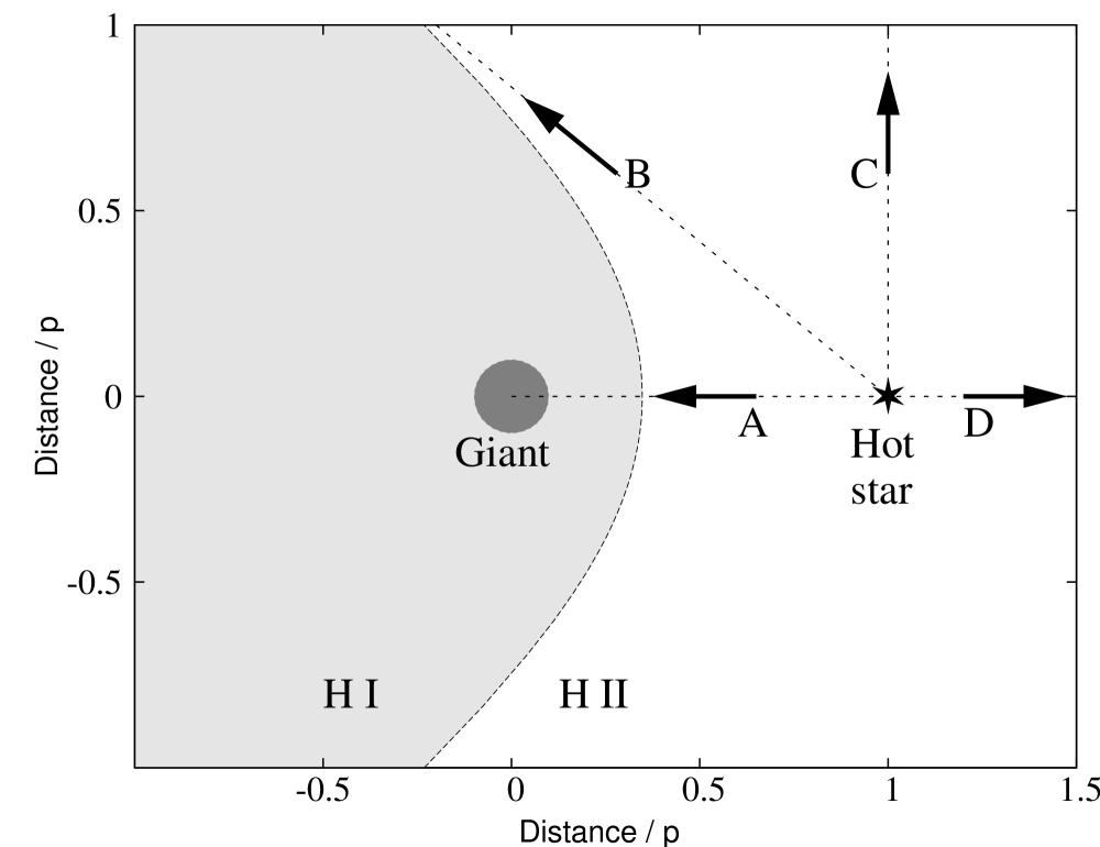
Figure 4: Top panel shows the ionization structure of AG Dra as seen pole-on. The HI/HII boundary was calculated according to Eq. (8) and $X=8$ (Sect. 4.2.). Bottom panel displays the corresponding function $\tau_{\rm e}(\varphi)$ for the orbital inclination of 60 and 90^∘. Labels A,B,C,D mark directions at specific orbital phases. Crosses correspond to $\tau_{\rm e}=0.044-0.078$, derived from the spectra during quiescent phase (Table 2).

Having defined the ionization structure in the binary, we can calculate the function $\tau_{\rm e}(\varphi)$ by integrating the electron concentration throughout the ionized zone along the line of sight to the hot star, i.e.

$$\tau_{\rm e}=\sigma_{\rm T}\int\limits_{0}^{s_{\theta}}n_{\rm e}(s){\rm d}s,$$ (12)

where the electron concentration $n_{\rm e}(s)=(1+a({\rm He}))n(r)$ and $n(r)$ is the density of hydrogen atoms in the wind from the giant. If the line of sight is not passing through the neutral region, $s_{\theta}\rightarrow\infty$ (in practice we adopted $s_{\theta}=100\times p$). To calculate correctly $\tau_{\rm e}(\varphi)$ for AG Dra, we considered its orbital inclination $i=60^{\circ}$ (Schmid & Schild, 1997). The function $\tau_{\rm e}(\varphi)$ is plotted in Fig. 4. A maximum value of $\tau_{\rm e}$ ($\sim$0.03) is around $\varphi=0.1$, when the line of sight passes the ionization region as an asymptote to the boundary (the direction B in the figure). A minimum of $\sim$0.007 corresponds to the position with the hot star in front ($\varphi=0.5$), because of the lowest densities of the wind from the giant. Figure 4 demonstrates that theoretical $\tau_{\rm e}(\varphi)$ function is significantly below the values derived from observations during quiescent phases (crosses in the figure, Table 2). This implies that the ionized fraction of the unperturbed wind from the giant is not capable of producing the observed electron scattering wings.

In a more realistic case the density distribution in a binary with mass-losing giant is determined mainly by the rotation of the binary and accretion by its compact companion, as was demostrated by several hydrodynamical simulations (e.g. Theuns & Jorissen, 1993; Bisikalo et al., 1995; Mastrodemos & Morris, 1998; Nagae et al., 2004). In these studies, it was shown that the regions with highly increased density around the accretor, around the mass-losing star and the whole binary, and behind the accretor (opposite to its orbital motion) were in the form of a disc, a spiralling arm and an elongated accretion wake, respectively. As a result, the column density of free electrons in the direction to the accretor can be enriched by the ionized material accumulated at/around the accretion disk at each position of the binary. Additional extremes can be expected for highly inclined orbits, when the line of sight passes throughout a higher density structure (see e.g. Fig. 6 of Dumm et al., 2000). A lower orbital inclination smooths out the density contrasts at different phases (see Fig. 2 of Theuns & Jorissen, 1993). Accordingly, in the real case, the faint electron-scattering wings during quiescent phases with $\tau_{\rm e}=0.044-0.078$ can be caused mainly by free electrons from/around the accretion disk and the ionized wind from the hot star, which corresponds to the total column density, $N_{\rm e}=\tau_{\rm e}/\sigma_{\rm T}\la 10^{23}$  cm^-2. The presence of the latter was proved by more authors (e.g. Vogel, 1993; Nussbaumer et al., 1995; Skopal, 2006).

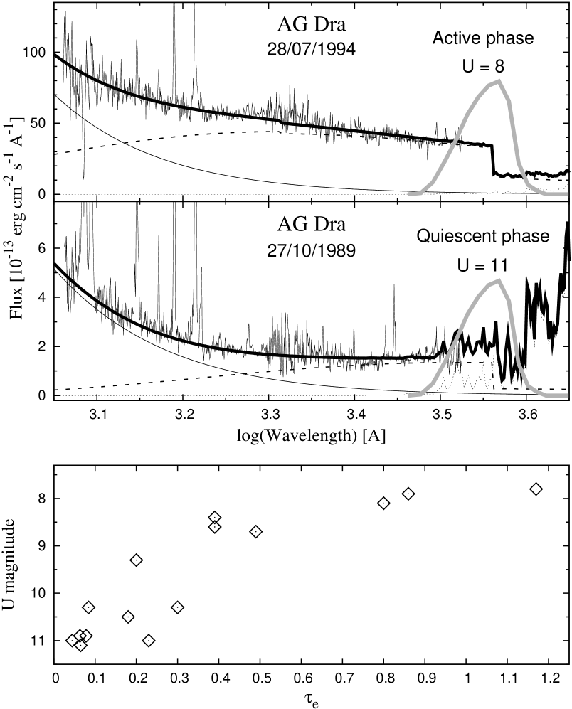
Figure 5: Top panels show the IUE spectra of AG Dra during the 1994 active phase (SWP51632+LWP28752) and a quiescent phase (SWP37473+LWP16675). The dashed, solid thin and dotted line represent the continuum from the nebula, the hot star and the giant, respectively. The solid thick line is their sum, the model SED (see Skopal, 2005, in detail). The gray line figures schematically the profile of the photometric $U$ filter. Bottom panel shows the dependence of $\tau_{\rm e}$ on the $U$-magnitude (Fig. 2, Table 2).

4.3 Thomson scattering during active phase

It is well known that during active phases the hot stars in symbiotic binaries enhance significantly the mass-loss rate (e.g. Fernández-Castro et al., 1995; Nussbaumer et al., 1995; Crocker et al., 2002; Skopal, 2006). The ejected material is ionized by the luminous central hot star, which thus enhances radiation from the symbiotic nebula. For example, Skopal (2005) derived a factor of $\approx$10 stronger nebular emission in the continuum during active phases with respect to values measured during quiescence. The enhanced mass-loss rate from the hot star thus represents a significant supplement of free electrons into the nebula. As a result, the electron optical depth, $\tau_{\rm e}=\sigma_{\rm T}N_{\rm e}$, will be considerably larger during active phases (Table 2). Here, this is well documented by the series of the AG Dra spectra (Fig. 2). The model SED demonstrates that the nebular radiation dominates also the spectral region of the photometric $U$ filter (see top panels of Fig. 5). Therefore, the level of the AG Dra activity is well mapped with the $U$ light curve (top panel of Fig. 2), which thus explains the relationship between $\tau_{\rm e}$ and the star’s brightness in $U$ (bottom panel of Fig. 5). A large scatter around $\tau_{\rm e}=0.2$ is probably connected with the transition phase, when the nebula can be partially optically thick in the continuum.

We can conclude that during active phases the large values of $\tau_{\rm e}=0.39-1.17$ (i.e. $N_{\rm e}=0.58-1.8\times 10^{24}$  cm^-2) are caused by a supplement of free electrons into the binary environment as a result of the enhanced mass-loss rate from the hot star.

5 Conclusions

We investigated the effect of Thomson scattering of the strong emission lines, OVI 1032 Å, 1038 Å and HeII 1640 Å, observed in the spectra of symbiotic stars AG Dra, Z And and V1016 Cyg. Our models of their profiles are in good agreement with those observed by FUSE, BEFS, TUES and IUE satellites (Figs. 2 and 3). This supports the idea that the broad wings of these lines result from the scattering of the line photons on free electrons. Their profile is given by two fitting parameters, $\tau_{\rm e}$ and $T_{\rm e}$ (Table 2), which characterize the scattering region, i.e. the symbiotic nebula. Particular results of our analysis can be summarized as follows.

1. The presence of the electron scattering wings in the line profiles of highly ionized elements locates their origin mostly to the vicinity of the hot star in the binary, with the highest density on the line of sight.

2. During quiescent phases, the mean $T_{\rm e}=19\,200\pm 2\,300$ K, while during active phases $T_{\rm e}=32\,300\pm 2\,000$ K. This findings agrees well with quantities derived independently by modelling the SED.

3. The electron optical depth also depends strongly on the star’s activity. During quiescent phases, $\tau_{\rm e}=0.056\pm 0.006$, while during active phases, $\tau_{\rm e}=0.64\pm 0.11$ (Table 2, Figs. 2 and 3). Uncertainties in the results given in (ii) and (iii) represent rms errors of the average values.

4. During quiescent phases, the ionized fraction of the wind from the giant within a simple (STB) model (Sect. 4.2) is not capable of giving rise a measurable effect of the Thomson scattering. In the real case, the faint electron-scattering wings with $\tau_{\rm e}=0.044-0.078$ are caused mainly by free electrons from/around the accretion disk and the ionized wind from the hot star with the total column density of a few $\times 10^{22}$  cm^-2 (Sect. 4.2., Fig. 4).

5. During active phases, the large values of $\tau_{\rm e}$ are caused by a supplement of free electrons into the nebula from the enhanced wind of the hot star, which increases $N_{\rm e}$ to $\sim 10^{24}$  cm^-2 (Sect. 4.3., Fig. 5).

The presumable relationship between $\tau_{\rm e}$ and the level of the activity, as suggested by our profile-fitting analysis, could be used in probing the mass-loss rate from the hot stars in symbiotic binaries.

References

- Belyakina (1985) Belyakina, T. S. 1985, IBVS, 2698
- Birriel et al. (2000) Birriel, J. J., Espey, B. R. & Schulte-Ladbeck, R. E. 2000, ApJ, 545, 1020
- Birriel (2004) Birriel, J. J. 2004, ApJ, 612, 1136
- Bisikalo et al. (1995) Bisikalo, D. V., Boyarchuk, A. A., Kuznetsov, O. A., Popov, Y. P., & Chechetkin, V. M. 1995, Astron. Reports, 39, 325
- Boyarchuk (1967) Boyarchuk, A. A. 1967, Soviet Astronomy, 11, 8
- Cardelli et al. (1989) Cardelli, J. A., Clayton G.C. & Mathis, J. S. 1989, ApJ, 345, 245
- Castor et al. (1970) Castor, J. I., Smith, L. F., & van Blerkom, D. 1970, ApJ, 159, 1119
- Corradi et al. (2003) Corradi, R. L. M., Mikolajewska, J., & Mahoney, T. J. 2003, Symbiotic Stars Probing Stellar Evolution, ASP Conf. Ser. 303 (San Francisco: ASP)
- Crocker et al. (2002) Crocker, M. M., Davis R. J., Spencer, R. E., et al. 2002, MNRAS, 335, 1100
- Dumm et al. (2000) Dumm, T., Folini, D., Nussbaumer, H., Schild, H., Schmutz, W., & Walder, R. 2000, A&A, 345, 1014
- Fekel et al. (2000) Fekel, F. C., Hinkle, K. H., Joyce, R. R. & Skrutskie, M.F. 2000, AJ, 120, 3255
- Fernandéz-Castro et al. (1988) Fernandéz-Castro, T., Cassatella, A., Gimenez, A., & Viotti, R. 1988, ApJ, 324, 1016
- Fernández-Castro et al. (1995) Fernández-Castro, T., González-Riestra, R., Cassatella, A., Taylor, A.R., & Seaquist E.R. 1995, ApJ, 442, 366
- Formiggini & Leibowitz (1994) Formiggini, L.; Leibowitz, E. M. 1994, A&A, 292, 534
- Greiner et al. (1997) Greiner, J. Bickert, K., Luthardt, R., Viotti, R., Altamore, A. Gonzalez-Riestra, R. & Stencel, R. E. 1997, A&A, 322, 576
- Hummer & Mihalas (1967) Hummer, D. G. & Mihalas, D. 1967, ApJ, 150, L57
- Isliker et al. (1989) Isliker, H., Nussbaumer, H., & Vogel, M. 1989, A&A, 219, 271
- Jung & Lee (2004) Jung, Y.-Ch., & Lee, H.-W. 2004, MNRAS, 350, 580
- Kenyon (1986) Kenyon, S. J. 1986, The Symbiotic Stars (Cambridge: Cambridge Univ. Press)
- Lee (2009) Lee, H.-W. 2009, MNRAS, 400, 2153
- Lee (2012) Lee, H.-W. 2012, ApJ, 750, 127
- Mastrodemos & Morris (1998) Mastrodemos, N., & Morris, M. 1998, ApJ, 497, 303
- McCuskey (1965) Mc Cuskey, S. 1965, IAUC. No. 1916
- Mihalas (1970) Mihalas, D. 1970, Stellar Atmosheres (San Francisco: W. H. Freeman), p. 321
- Mikolajewska et al. (1995) Mikolajewska, J., Kenyon, S. J., Mikolajewski, M., et al. 1995, AJ, 109, 1289
- Mikolajewska et al. (2002) Mikolajewska, J., Ivison, R. J., & Omont, A. 2002, Adv. Space Res., 30, 2045
- Münch (1950) Münch, G. 1950, ApJ, 112, 266
- Mürset et al. (1991) Mürset, U., & Nussbaumer, H., Schmid, H.M. & Vogel, M. 1991, A&A, 248, 458
- Mürset & Schmid (1999) Mürset, U. & Schmid, H. M. 1999, A&A, 137, 473
- Nagae et al. (2004) Nagae, T., Oka, K., Matsuda, T., Fujiwara, H., Hachisu, I., & Boffin, H. M. J. 2004, A&A, 419, 335
- Nussbaumer & Schild (1981) Nussbaumer, H. & Schild, H. 1981, A&A, 101, 118
- Nussbaumer & Vogel (1987) Nussbaumer, H. & Vogel, M. 1987, A&A, 182, 51
- Nussbaumer et al. (1989) Nussbaumer, H., Schmid, H. M., & Vogel, M. 1989, A&A, 211, L27
- Nussbaumer et al. (1995) Nussbaumer, H., Schmutz, W., & Vogel, M. 1995, A&A, 293, L13
- Parimucha et al. (2002) Parimucha, Š., Chochol, D., Pribulla, T., Buson, L. M., & Vittone, A. A. 2002, A&A, 391, 999
- Rogerson & Ewell (1984) Rogerson, J. B., & Ewell, M. W. 1984, ApJS, 58, 265
- Rosswog & Brüggen (2007) Rosswog, S., & Brüggen, M. 2007, Introduction to High-Energy Astrophysics (Cambridge: Cambridge Univ. Press)
- Schmid (1998) Schmid, H.M. 1998, Reviews in Modern Astronomy, 11, 297
- Schmid & Schild (1997) Schmid, H.M. & Schild, H. 1997, A&A, 321, 791
- Schmid et al. (1999) Schmid, H. M., Krautter, J., Appenzeller, I., et al. 1999, A&A, 348, 950
- Schröder (1985) Schröder, K. P. 1985, A&A, 147, 103
- Seaquist, Taylor & Button (1984, hereafter STB) Seaquist, E. R., Taylor, A. R., & Button, S. 1984, ApJ, 284, 202 (STB)
- Skopal (2005) Skopal, A. 2005, A&A, 440, 995
- Skopal (2006) Skopal, A. 2006, A&A, 457, 1003
- Skopal et al. (2006) Skopal, A., Vittone, A. A., Errico, L., et al. 2006, A&A, 453, 279
- Skopal et al. (2009) Skopal, A., Sekeráš, M., González-Riestra, R., & Viotti, R. F. 2009, A&A, 507, 1531
- Skopal et al. (2012) Skopal, A., Shugarov, S., Vaňko, M., et al., 2012, Astron. Nachr., 333, 242
- Theuns & Jorissen (1993) Theuns, T., & Jorissen, A. 1993, MNRAS, 265, 946
- Vogel (1993) Vogel, M. 1993, 274, L21
- Young et al. (2005) Young, P. R., Dupree, A. K., Espey, B. R., Kenyon, S. J., & Ake, T. B. 2005, ApJ, 618, 891