Photo-production of Bound States with Hidden Charms

Abstract

The photo-production of $J/\Psi$-${}^{3}He$ bound state ($[^{3}He]_{J/\Psi}$) on a ${}^{4}He$ target has been investigated using the impulse approximation. The calculations have been performed using several $\gamma+N\rightarrow J/\Psi+N$ models based on the Pomeron-exchange and accounting for the pion-exchange mechanism at low energies. The $J/\Psi$ wavefunctions in $[^{3}He]_{J/\Psi}$ are generated from various $J/\Psi$-nucleus potentials which are constructed by either using a procedure based on the Pomeron-quark coupling mechanism or folding a $J/\Psi$-N potential ($v_{J/\Psi,N}$) into the nuclear densities. We consider $v_{J/\Psi,N}$ derived from the effective field theory approach, Lattice QCD, and Pomeron-quark coupling mechanism. The upper bound of the predicted total cross sections is about $0.1-0.3$ pico-barn. We also consider the possibility of photo-production of a six quark-$J/\Psi$ bound state ($[q^{6}]_{J/\Psi})$ on the ${}^{3}He$ target. The Compound Bag Model of $NN$ scattering and the quark cluster model of nuclei are used to estimate the $[q^{6}]$-N wavefunction in ${}^{3}He$ by imposing the condition that the calculated ${}^{3}He$ charge form factor must be consistent with what is predicted by the conventional nuclear model. The upper bound of the predicted total cross sections of $\gamma+^{3}He\rightarrow[q^{6}]_{J/\Psi}+N$ is about 2 - 4 pico-barn, depending on the model of $\gamma+N\rightarrow J/\Psi+N$ used in the calculations. Our results call for the need of precise measurements of $\gamma+p\rightarrow J/\Psi+p$ and also the $\gamma+^{2}H\rightarrow J/\Psi+n+p$ reactions near the threshold.

I introduction

The role of the gluon field in determining the interactions between nucleons and quark-antiquark ($Q\bar{Q}$) systems, which do not share the same $up$ and $down$ quarks with the nucleon, is one of the interesting subjects in understanding Quantum Chromodynamics(QCD). An important step toward this direction was taken by Peskinpesk79 who applied the methodology of the operator product expansion to evaluate the strength of the color field emitted by heavy $Q\bar{Q}$ systems. His results suggestedbp79 that the van der Waals force induced by the color field of $J/\Psi$ on nucleons can generate an attractive short-range $J/\Psi$-$N$ interaction. By using the effective field theory method, Luke, Manohar, and Savageluke92 used the results from Peskin to predict the $J/\Psi$-nucleon forward scattering amplitude which was used to get an estimation that $J/\Psi$ can have a few MeV/nucleon attraction in nuclear matter. Brodsky and Millerbrodsky-1 further investigated the $J/\Psi$-N forward scattering amplitude of Ref.luke92 to derive a $J/\Psi$-N potential ($v_{J/\Psi,N}$) which gives an $J/\Psi$-N scattering length of -$0.24$ fm. The result of Peskin was also used by Kaidalov and Volkovitskyrussia , who differed from Ref.brodsky-1 in evaluating the gluon content in the nucleon, to give a much smaller scattering length of -$0.05$ fm. In a Lattice QCD calculation, Kawanai and Saskilqcd obtained an attractive $J/\Psi$-N potential $v_{J/\Psi,N}=$ - $\alpha e^{-\mu r}/{r}$ with $\alpha=0.1$ and $\mu=0.6$ GeV, which gives a scattering length - $0.09$ fm. In Ref.brodsky90 , Brodsky, Schmidt and de Teramond proposed an approach to calculate the potential between a $c\bar{c}$ meson and a nucleus by using the Pomeon-exchange model of Dannachie and Lanshoffdonn84 . The $J/\Psi$-N potential obtained in this approach is $v_{J/\Psi,N}=$ - $\alpha e^{-\mu r}/{r}$ with $\alpha=0.6$ and $\mu=0.6$ GeV which gives a rather large scattering length - $8.83$ fm.

Our first objective in this paper is to explore whether these $J/\Psi$-N potentials, with rather different attractive strengths, can form $J/\Psi$-nucleus bound states. Following the well developed method in nuclear reaction theoryfeshbach-1 , this is done by searching for bound states by solving the Schrodinger equation with a folding potential constructed by integrating the $J/\Psi$-N potential over the nuclear density. We will also consider the approach of Ref.brodsky90 in predicting $J/\Psi$-nucleus bound states by the coherent sum of Pomeon-exchange between quarks in $J/\Psi$ and all quarks in the nucleus. For each of the predicted bound $[^{3}He]_{J/\Psi}$ systems, we then estimate the photo-production cross section of the $\gamma+^{4}He\rightarrow[^{3}He]_{J/\Psi}+N$ reaction to facilitate future experimental investigationsworkshop .

The second part of this work is motivated by the investigations by Brodsky and de Teramondbrodsky-3 who found that the spin correlation of $pp$ elastic scattering near the $J/\Psi$ production threshold can be explained if one postulates the excitation of a hidden charm ($c$) state $|qqqqqqc\bar{c}>$. Based on the similar consideration on the role of multi-quark configurations, Brodsky, Chudakov, Hoyer, and Lagetbrodsky-2 suggested in a study of $\gamma+^{2}H\rightarrow J/\Psi+n+p$ reaction that $J/\Psi$ can interact strongly with the six-quark $[q^{6}]$ component of the deuteron wavefunction because the octet 3-quark $[q^{3}]_{8}$ in the $[q^{6}]$ can directly interact with each quark in $J/\Psi$. These two works suggest the possibility that if $J/\Psi$ overlap with a $[q^{6}]$ cluster in nuclei, a bound $[q^{6}]_{J/\Psi}$ system could be formed. It is of course very difficult, if not impossible, to estimate $[q^{6}]$-${J/\Psi}$ interaction. Instead, we will simply assume the existence of such states and use the previous workslow ; mulder ; itep ; fasano-1 ; fasano-2 ; bakker ; vary ; japan-he3 on quark clusters in nuclei to explore how the cross sections of $\gamma+^{3}He\rightarrow[q^{6}]_{J/\Psi}+N$ depend on the parameters characterizing the $[q^{6}]$-${J/\Psi}$ interaction within a potential model.

Our first task is to construct a model of $\gamma+N\rightarrow J/\Psi+N$ reaction. At high energies, it is well recognized that this reaction can be described by the Pomeron-exchange model with an interpretationdonn84 ; LN87 ; LM95 ; PL97 that Pomeron-exchange is due to the exchange of gluons within QCD. This is illustrated in part (a) of Fig.1. At low energies, one expects that mechanisms other than Pomeron-exchange could also contribute as can be seen in the exclusive $\phi$ photo-production reaction on the nucleonPL97 ; titov-lee ; ky12 . However, very little investigation has been done for $J/\Psi$ photo-production in the near threshold region. As a first step, we will only consider the meson-exchange mechanism which can be calculated from using the partial decay width of $J/\Psi\to\pi\rho$ listed by Particle Data Grouppdg (PDG). With the vector meson dominance (VDM) assumption, this observed decay process indicates that $J/\Psi$ photo-production can also be due to the exchanges of a $\pi$ meson with the nucleon, as illustrated in part (b) of Fig.1.

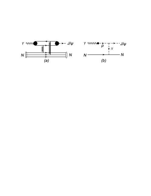
Figure 1: Reaction mechanisms of $\gamma N\rightarrow J/\Psi+N$ : (a) Pomeron-exchange, (b) pion-exchange.

We next consider the photo-nuclear reaction mechanism that a $J/\Psi$ is produced from a nucleon in a nucleus with mass number $A$ and then forms a bound state with the spectator $B$ system which can be a $(A-1)$ nuclear system or a quark cluster $[q^{3(A-1)}]$ in the target nucleus $A$. With this commonly used impulse approximation, the reaction cross sections can be calculated from the $\gamma+N\rightarrow J/\Psi+N$ amplitude, which will be generated from the Pomeron-exchange and pion-exchange mechanisms described above, and the initial nucleon and final $J/\Psi$ wavefunctions. The nucleon wavefunctions can be taken from the available nuclear models. The $J/\Psi$ wavefunctions will be generated from various $J/\Psi$-$B$ potentials mentioned above. For simplicity, we only present the predictions of the cross sections of $\gamma+[^{4}He]\rightarrow N+[^{3}He]_{J/\Psi}$ and $\gamma+[^{3}He]\rightarrow N+[q^{6}]_{J/\Psi}$ reactions.

In section II, we present formula for calculating the $\gamma+N\rightarrow J/\Psi+N$ amplitudes from the Pomeron-exchange and pion-exchange mechanisms. The impulse approximation formula for calculating the cross sections of $\gamma+[A]\rightarrow[B]_{J/\Psi}+N$ are given in section III. Our results are presented in section IV. In section V, we give a summary and discuss the necessary future work.

II Formula for $\gamma+N\rightarrow J/\Psi+N$ reaction

In the center of mass system, the differential cross section of $\gamma(\vec{q})+N(-\vec{q})\rightarrow J/\Psi(\vec{k})+N(-\vec{k})$ with invariant mass $W$ can be written

$$\frac{d\sigma}{d\Omega} = [\frac{(2\pi)^{4}E_{N}(q)}{W}][\frac{kE_{J/\Psi}(k)E_{N}(k)}{W}]\frac{1}{4}\sum_{\lambda_{\gamma},\lambda_{J/\Psi}}\sum_{m_{s},m^{\prime}_{s}}|<\vec{k}\lambda_{J/\Psi}m^{\prime}_{s}|t(W)|\vec{q}\lambda_{\gamma}m_{s}>|^{2}\,,$$ (1)

where $\lambda_{J/\Psi}$ and $\lambda_{\gamma}$ are the helicities of the $J/\Psi$ and photon, respectively, $m_{s}$ is the z-component of the nucleon spin, and $E_{a}(p)=[m^{2}_{a}+\vec{p}^{\,\,2}]^{1/2}$ is the energy of a particle with mas $m_{a}$. The reaction amplitude is written as

$$<\vec{k}\lambda_{J/\Psi}m^{\prime}_{s}|t(W)|\vec{q}\lambda_{\gamma}m_{s}> = \frac{1}{(2\pi)^{3}}\frac{1}{\sqrt{2E_{J/\Psi}(k)}}\sqrt{\frac{m_{N}}{E_{N}(k)}}\sqrt{\frac{m_{N}}{E_{N}(q)}}\frac{1}{\sqrt{2q}}$$ (2)

$$\times[\bar{u}_{m^{\prime}_{s}}(p^{\prime})\epsilon^{*}_{\mu}(k,\lambda_{J/\Psi})M^{\mu\nu}(p^{\prime},p)\epsilon_{\nu}(q,\lambda_{\gamma})u_{m_{s}}({p})]\,,$$

where $u_{m_{s}}({p})$ is the nucleon spinor (with the normaliztion $\bar{u}_{m_{s}}({p}){u}_{m^{\prime}_{s}}({p})=\delta_{m_{s},m^{\prime}_{s}}$) , $\epsilon_{\mu}(k,\lambda_{J/\Psi})$ and $\epsilon_{\nu}(q,\lambda_{\gamma})$ are the polarization vectors of $J/\Psi$ and photon, respectively. Here we also have introduced the four-momenta for the initial and final nucleons:

$$p = (E_{N}(q),-\vec{q})\,\,\,\,\,;\,\,\,p^{\prime}=(E_{N}(k),-\vec{k})\,.$$

In the following subsections, we give formula for calculating the invariant amplitude $M^{\mu\nu}$ due to the Pomeron-exchange and meson-exchange mechanisms, as illustrated in Fig.1.

II.1 Pomeron-exchange amplitude

Within the Pomeron-exchange model of Donnachie and Landshoff donn84 , the vector meson photo-production at high energies is due to the mechanism that the incoming photon couples with a $q\bar{q}$ pair which interacts with the nucleon by the Pomeron exchange before forming the outgoing vector meson. The quark-Pomeron vertex is obtained by the Pomeron-photon analogydonn84 , which treats the Pomeron as a $C=+1$ isoscalar photon, as suggested by a study of non perturbative two-gluon exchanges LN87 . Following the formula given explicitly in Ref.OL02 , we then have

$$\mathcal{M}^{\mu\nu}_{\mathbb{P}}(p^{\prime},p)=G_{\mathbb{P}}(s,t)\mathcal{T}^{\mu\nu}_{\mathbb{P}}(p^{\prime},p)$$ (3)

with

$$\mathcal{T}^{\mu\nu}_{\mathbb{P}}(p^{\prime},p)=i12\sqrt{4\pi\alpha_{\rm em}}\frac{M_{V}^{2}\beta_{q}\beta_{q^{\prime}}}{f_{V}}\frac{1}{M_{V}^{2}-t}\left(\frac{2\mu_{0}^{2}}{2\mu_{0}^{2}+M_{V}^{2}-t}\right)F_{1}(t)\{k\!\!\!/\,g^{\mu\nu}-k^{\mu}\gamma^{\nu}\}\,,$$ (4)

where $t=(p-p^{\prime})^{2}$, $s=(q+p)^{2}=W^{2}$, $\alpha_{\rm em}=e^{2}/4\pi$, $\beta_{q}$ is the Pomeron-quark coupling constant, $M_{V}$ is the vector meson mass, and $F_{1}(t)$ is the isoscalar electromagnetic form factor of the nucleon,

$$F_{1}(t)=\frac{4M_{N}^{2}-2.8t}{(4M_{N}^{2}-t)(1-t/0.71)^{2}}.$$ (5)

Here $t$ is in unit of GeV², and $M_{N}$ is the proton mass.

The Regge propagator for the Pomeron in Eq. (3) is

$$G_{\mathbb{P}}=\left(\frac{s}{s_{0}}\right)^{\alpha_{P}(t)-1}\exp\left\{-\frac{i\pi}{2}\left[\alpha_{P}(t)-1\right]\right\}\,,$$ (6)

where $\alpha_{P}(t)=\alpha_{0}+\alpha^{\prime}_{P}t$. It is commonOL02 to use $\alpha_{0}=1.08$ and $\alpha^{\prime}_{P}=1/s_{0}=0.25$ GeV^-2. In Eq. (4), $f_{V}$ is the vector meson decay constant: $f_{\rho}=5.33$, $f_{\omega}=15.2$, $f_{\phi}=13.4$, and $f_{J/\Psi}=11.2$. The other parameters in Eq.(4) have been determined by fittingOL02 the total cross section data of the photo-production of $\rho$ and $\omega$ : $\beta_{u}=\beta_{d}=2.07$ GeV^-1 and $\mu_{0}^{2}=1.1$ GeV².

With the parameters specified above, our task is to examine the extent to which the total cross section of photo-production of $J/\Psi$ can be fitted by only adjusting the Pomeron-charmed quark coupling constant $\beta_{c}$. This will be discussed in section IV.

II.2 Pion-exchange amplitude

We observe from Particle Datapdg that the width of the $J/\Psi\to\pi^{0}\rho^{0}$ is significant,

$$\Gamma_{J/\Psi\rightarrow\pi^{0}\rho^{0}}=0.92\,\,\,MeV\,\,\,\times(0.56\pm 0.07)\%\,.$$ (7)

With the vector meson dominance (VDM) assumption, this experimental information allows us to calculate the one-pion-exchange amplitude of $\gamma+N\rightarrow J/\Psi+N$, as illustrated in Fig.1(b), by using the following Lagrangian

$$L=L_{J/\Psi,\rho^{0}\pi^{0}}+L_{\pi NN}+L_{VDM}$$ (8)

with

$$L_{J/\Psi,\rho^{0}\pi^{0}} = -\frac{g_{J/\Psi,\rho^{0}\pi^{0}}}{m_{J/\Psi}}\epsilon^{\mu\nu\alpha\beta}\partial_{\mu}{\rho^{0}}_{\nu}\partial_{\alpha}\phi_{J/\Psi,\beta}{\phi}_{\pi^{0}}\,,$$ (9)

$$L_{\pi NN} = -\frac{f_{\pi NN}}{m_{\pi}}\bar{\psi}_{N}\gamma_{\mu}\gamma_{5}\vec{\tau}\psi_{N}\partial^{\mu}\cdot\vec{\phi}_{\pi}\,,$$ (10)

$$L_{VDM} = \frac{em_{\rho}}{f_{\rho}}A^{\mu}\rho^{0}_{\mu}\,,$$ (11)

where $\rho^{0}_{\mu}$, $\phi_{J/\Psi,\beta}$, $\vec{\phi}_{\pi}$, $A^{\mu}$, and $\psi_{N}$ are the field operators for $\rho^{0}$, $J/\Psi$, $\pi$, photon ($\gamma$), and nucleon ($N$), respectively. The mass for particle $a$ is denoted as $m_{a}$. The well determined coupling constants are $f^{2}_{\pi NN}/4\pi=0.079$, $e^{2}/4\pi=1/137$, and $f_{\rho}=5.33$. To determine $g_{J/\Psi,\rho^{0}\pi^{0}}$, we use $L_{J/\Psi,\rho^{0}\pi^{0}}$ given in Eq.(9) to calculate the decay width

$$\Gamma_{J/\Psi\rightarrow\pi^{0}\rho^{0}} = (2\pi)\frac{1}{3}\sum_{\lambda_{\rho},\lambda_{J/\Psi}}\int d\Omega_{k}|<\vec{k}\lambda_{\rho}|H|\vec{p}=0,\lambda_{J/\Psi}>|^{2}\frac{kE_{\pi}(k)E_{\rho}(k)}{m_{J/\Psi}}\,,$$ (12)

where $k$ is defined by $m_{J/\Psi}=E_{\pi}(k)+E_{\rho}(k)$, and

$$<\vec{k}\lambda_{\rho}|H|\vec{\vec{p},\lambda_{J/\Psi}}> = \frac{1}{(2\pi)^{3/2}}\frac{1}{\sqrt{2E_{J/\Psi}(p)}}\frac{1}{\sqrt{2E_{\rho}(k)}}\frac{1}{\sqrt{2E_{\pi}(k)}}$$ (13)

$$\times\epsilon^{\mu\nu\alpha\beta}k^{\rho}_{\mu}\epsilon_{\nu,\lambda_{\rho}}(k^{\rho})p_{\alpha}\epsilon_{\beta,\lambda_{J/\Psi}}(p)[\frac{\Lambda^{2}_{J/\Psi}}{(\vec{k}^{2}+\Lambda^{2}_{J/\Psi})}]^{2}\,.$$

Here we have included a dipole cutoff function with a range parameter $\Lambda_{J/\Psi}$. The four-momenta are defined in the rest frame of $J/\Psi$:

$$p = (m_{J/\Psi},\vec{0})\,,$$

$$k^{\rho} = (E_{\rho}(k),\vec{k})\,,$$

$$k^{\pi} = (E_{\pi}(k),-\vec{k})\,.$$

By using Eqs.(12)-(13) and the experimental value given in Eq.(7), we find $g_{J/\Psi,\pi^{0}\rho^{0}}=0.032$ for a cutoff $\Lambda_{J/\Psi}=2000$ MeV.

With the Lagrangian Eq.(8), the one-pion-exchange invariant amplitude for $\gamma(q)+N(p)\rightarrow J/\Psi(k)+N(p^{\prime})$ can be written as

$$I_{fi}=\bar{u}_{m^{\prime}_{s}}(p^{\prime})\epsilon^{*}_{\mu}(k,\lambda_{J/\Psi})M^{\mu\nu}_{\pi}(p^{\prime},p)\epsilon_{\nu}(q,\lambda_{\gamma})u_{m_{s}}(p)$$ (14)

with

$$M^{\mu\nu}_{\pi}(p^{\prime},p) = G\times F(t)\frac{1}{t-m^{2}_{\pi}}\epsilon^{\mu\nu\alpha\beta}k_{\alpha}q_{\beta}[\gamma\cdot(p^{\prime}-p)]\,,$$ (15)

where $t=(p-p^{\prime})^{2}$, and

$$G = \frac{e}{f_{\rho}}\frac{g_{J/\Psi,\rho^{0}\pi^{0}}}{m_{J/\Psi}}\frac{f_{\pi NN}}{m_{\pi}}\,,$$ (16)

$$F(t) = F_{\pi NN}(t)F_{J/\Psi,\rho^{0}\pi^{0}}(t)\,.$$ (17)

Here we have introduced a cutoff form factor $F(t)$ to regularize the interaction verteces. For simplicity, we use the following form

$$F(t)=\left(\frac{\Lambda^{2}}{\Lambda^{2}-t}\right)^{n}\,.$$ (18)

We set $n=4$, and $\Lambda=\Lambda_{J/\Psi}=2000$ MeV.

III Photo-production of $[B]_{J/\Psi}$ bound state

III.1 Reaction Mechanism

With the impulse approximation, we assume that a $J/\Psi$ is produced on a nucleon in the target nucleus $A$ and then is attracted by a spectator system $B$ to form a bound state $[B]_{J/\Psi}$. For simplicity, $[B]_{J/\Psi}$ is denoted as $d$ in the following formula.

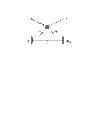
Figure 2: The impulse approximation mechanism of $\gamma+A\rightarrow N+[B]_{J/\Psi}$ reaction. $A$ is a nucleus with mass number $A$ and $B$ could be a nucleus with mass number $(A-1)$ or a $[q^{3(A-1)}]$ multi-quark cluster.

With the mechanism illustrated in Fig.2, the cross section of $\gamma(\vec{q})+A(-\vec{q})\rightarrow N(\vec{p})+d(-\vec{p})$ in the center of mass system can be written as

$$\frac{d\sigma}{d\Omega} = [\frac{(2\pi)^{4}E_{A}(q)}{W}][\frac{pE_{N}(p)E_{d}(p)}{W}]$$ (19)

$$\times\frac{1}{2}\frac{1}{2J_{A}+1}\sum_{\lambda,M_{J_{A}}}\sum_{m_{s},m_{d}}|<\vec{p}m_{s},\Psi_{j_{d}M_{d}}|T(W)|\vec{q}\lambda,\Phi^{A}_{J_{A},M_{J_{A}}}>|^{2}\,,$$

where

$$<\vec{p}m_{s},\Psi_{j_{d}M_{d}}|T(W)|\vec{q}\lambda,\Phi^{A}_{J_{A},M_{J_{A}}}>=\sum_{j,m_{j}}\sum_{j_{\alpha},m_{j_{\alpha}}}<\Psi_{j_{d}M_{d}}|a^{\dagger}_{jm_{j}}b_{j_{\alpha},m_{j_{\alpha}}}|\Phi^{A}_{J_{A},M_{J_{A}}}>$$

$$\times[\sum_{m_{J/\Psi},m_{s_{\alpha}}}\int d\vec{k}\chi^{*}_{j,m_{j}}(\vec{Q}_{d},m_{J/\Psi})<\vec{p}m_{s},\vec{k}m_{J/\Psi}|t(W)|\vec{q}\lambda,\vec{p}_{\alpha}m_{s_{\alpha}}>\phi_{j_{\alpha},m_{j_{\alpha}}}(\vec{Q}_{A},m_{s_{\alpha}})\,.$$

(20)

Here $a^{\dagger}_{jm_{j}}$ is the creation operator for a $J/\Psi$ with wavefunction $\chi_{j,m_{j}}(\vec{Q}_{d},m_{J/\Psi})$, $b_{j_{\alpha},m_{j_{\alpha}}}$ an annihilation operator for a nucleon with wavefunction $\phi_{j_{\alpha},m_{\alpha}}(\vec{Q}_{A},m_{s_{\alpha}})$, and the $\gamma+N\rightarrow J/\Psi+N$ amplitude is

$$<\vec{p}m_{s},\vec{k}m_{J/\Psi}|t(W)|\vec{q}\lambda,\vec{p}_{\alpha}m_{s_{\alpha}}> = \frac{1}{(2\pi)^{3}}\frac{1}{\sqrt{2E_{J/\Psi}(k)}}\sqrt{\frac{m_{N}}{E_{N}(p_{\alpha})}}\frac{1}{\sqrt{2q}}\sqrt{\frac{m_{N}}{E_{N}(p)}}$$

$$\times[\bar{u}_{m_{s}}(p)\epsilon^{*}_{\mu}(k,m_{J/\Psi})\{M^{\mu\nu}_{\pi}(p,p_{\alpha})+\mathcal{M}^{\mu\nu}_{\mathbb{P}}(p,p_{\alpha})\}$$

$$\,\,\times\epsilon_{\nu}(q,\lambda)u_{m_{s_{\alpha}}}(p_{\alpha}))]\,,$$

where $M^{\mu\nu}_{\pi}$ is the pion-exchange amplitude given in Eq.(15), and $\mathcal{M}^{\mu\nu}_{\mathbb{P}}$ is the Pomeron-exchange amplitude in Eq.(3).

For simplicity, we will only perform calculations for the reactions on ${}^{3}He$ and ${}^{4}He$. For estimations of cross sections on these target nuclei, it is sufficient to use the s-wave harmonic oscillator wavefunctions for both the target $A$ and $B$ in the $[B]_{J/\Psi}$ bound state. We also only consider the case that the $J/\Psi$ in the produced bound $B_{J/\Psi}$ is on an s-wave orbital. For the case $B=A-1$ nuclear system, we thus write the initial ($|\Phi^{A}>$) and final ($|\Psi>$) nuclear states as

$$|\Phi^{A}> = [|N>\otimes|\Phi^{A-1}>]_{L=0}\,,$$ (22)

$$|\Psi> = [|J/\Psi>\otimes|\Phi^{A-1}>]_{L=0}\,,$$ (23)

where $L$ is the relative angular momentum between $N$ or $J/\Psi$ and the $(A-1)$ nucleus. Explicitly, we have

$$|\Phi^{A}_{J_{A},M_{J_{A}}}> = \sum_{M_{J_{A-1}}}\sum_{j_{\alpha},m_{j_{\alpha}}}<J_{A}M_{J_{A}}|j_{\alpha}J_{A-1}m_{j_{\alpha}}M_{J_{A-1}}>b^{\dagger}_{j_{\alpha}m_{j_{\alpha}}}|\Phi^{A-1}_{J_{A-1},M_{J_{A-1}}}>\,,$$

$$|\Psi_{J_{d},M_{J_{d}}}> = \sum_{M_{J_{A-1}}}\sum_{j,m_{j}}<J_{d}M_{d}|jJ_{A-1}m_{j}M_{J_{A-1}}>a^{\dagger}_{jm_{j}}|\Phi^{A-1}_{J_{A-1},M_{J_{A-1}}}>\,.$$ (24)

Then the momentum variables in Eqs.(20) and (LABEL:eq:t-mx) are

$$\vec{p}_{\alpha} = \vec{p}+\vec{k}-\vec{q}\,,$$ (25)

$$\vec{p}_{\beta} = -\vec{p}-\vec{k}=-\vec{q}-\vec{p}_{\alpha}\,,$$ (26)

$$\vec{Q}_{A} = \frac{\vec{p}_{\alpha}E_{A-1}(\vec{p}_{\beta})-\vec{p}_{\beta}E_{N}(\vec{p}_{\alpha})}{E_{A-1}(\vec{p}_{\beta})+E_{N}(\vec{p}_{\alpha})}\,,$$ (27)

$$\vec{Q}_{d} = \frac{\vec{k}E_{A-1}(\vec{p}_{\beta})-\vec{p}_{\beta}E_{J/\Psi}(\vec{k})}{E_{J/\Psi}(\vec{k})+E_{A-1}(\vec{p}_{\beta})}\,,$$ (28)

where $\vec{Q}_{d}$ ($\vec{Q}_{A}$) is the relativistic relative momentum between $J/\Psi$ ($N)$ and the $(A-1)$ nuclear system.

For the target ${}^{4}He$, we have $J_{A}=0$ and assume that $|\Phi^{A-1}_{J_{A-1},M_{J_{A-1}}}>$ is the ${}^{3}He$ ground state with $J_{A-1}=1/2$. We then have the following simplicities:

$$<\Psi_{j_{d}M_{d}}|a^{\dagger}_{jm_{j}}b_{j_{\alpha},m_{j_{\alpha}}}|\Phi^{A}_{J_{A},M_{J_{A}}}> = <J_{A}M_{J_{A}}|j_{\alpha}J_{A-1}m_{j_{\alpha}}M_{J_{A-1}}><J_{d}M_{d}|jJ_{A-1}m_{j}M_{J_{A-1}}>$$ (29)

$$\rightarrow \frac{1}{\sqrt{2}}<J_{d}M_{J_{d}}|j_{\alpha}j-m_{j_{\alpha}}m_{j}>\,,$$

and

$$\chi_{j,m_{j}}(\vec{Q}_{d},m_{J/\Psi}) = \delta_{j,1}\delta_{m_{j},m_{J/\Psi}}\frac{1}{\sqrt{4\pi}}F({Q}_{d})\,,$$ (30)

$$\phi_{j_{\alpha},m_{j_{\alpha}}}(\vec{Q}_{A},m_{s_{\alpha}}) = \delta_{j_{\alpha},1/2}\delta{m_{j_{\alpha}},m_{s_{\alpha}}}\frac{1}{\sqrt{4\pi}}R({Q}_{A})\,,$$ (31)

Eq.(20) then becomes

$$<\vec{p}m_{s},\Psi_{j_{d}M_{d}}|T(W)|\vec{q}\lambda,\Phi^{A}_{J_{A},M_{J_{A}}}>$$

$$=\sum_{M_{J_{A-1}}}\sum_{m_{J/\Psi},m_{s_{\alpha}}}<J_{A}M_{J_{A}}|j_{\alpha}J_{A-1}m_{j_{\alpha}}M_{J_{A-1}}><J_{d}M_{d}|jJ_{A-1}m_{j}M_{J_{A-1}}>$$

$$\times[\int d\vec{k}\frac{1}{\sqrt{4\pi}}F({Q}_{d})<\vec{p}m_{s}\vec{k}m_{J/\Psi}|t(W)|\vec{q}\lambda,\vec{p}_{\alpha}m_{s_{\alpha}}>\frac{1}{\sqrt{4\pi}}R({Q}_{A})]\,.$$ (32)

We have applied the formula Eqs.(19) and (32) to estimate the production cross section on ${}^{4}He$. We use the usual s-wave harmonic oscillator wavefunction with $b=1.32$ fm for the target ${}^{4}He$

$$R(p)=[Ne^{\frac{-b^{2}p^{2}}{2}}]$$ (33)

with the normalization $\int R^{2}(p)p^{2}dp=1$. For the $J/\Psi$ wavefunction in $d=[^{3}He]_{J/\Psi}$, we will generate a s-wave $\psi_{J/\Psi}(r)$ from a potential $V_{J/\Psi,B}(r)$ with the normalization $\int r^{2}dr|\psi_{J/\Psi}(r)|^{2}=1$. The wavefunction in Eq.(30) and also in (32) can then be calculated from

$$F(p) = \int_{0}^{\infty}r^{2}drj_{0}(pr)\psi_{J/\Psi}(r)\,,$$ (34)

where $j_{0}(z)$ is the spherical Bessel function. The form of $V_{J/\Psi,B}(r)$ will be discussed in section IV.

The above formula can be easily extended to investigate other possible impulse approximation mechanisms as far as all wavefucnctions in the bound $A$ and $[B]_{J/\psi}$ are all in s waves. This is what we will need in section IV when we consider the production of $[q^{6}]_{J/\Psi}$ from the $q^{6}$-N component of ${}^{3}He$.

IV Results

IV.1 Models of $\gamma+N\rightarrow J/\Psi+N$ reaction

We first develop a model consisting of Pomeron-exchange and pion-exchange mechanisms, as described in section II. With the parameters specified there, we try to fit the available total cross section data of $\gamma+p\rightarrow J/\Psi+p$ up to invariant mass $W=300$ GeV by only adjusting the charmed quark-Pomeron coupling constant $\beta_{c}$. With $\beta_{c}=1.21$ we only able to fit the data up to 20 GeV. Clearly, the result at high energy is not satisfactory as shown in the red dashed curve in the left-hand side of Fig.3. We then find that by changing $\alpha_{0}$ of the Regge trajectory in the Pomeron propagator Eq.(6) from $\alpha_{0}=1.08$, as determined in the previous fitsOL02 to the total cross sections of $\rho$ and $\omega$ photo-production, to $\alpha_{0}=1.25$, we are able to get a very good fit to the data by choosing $\beta_{c}=0.84$ GeV^-1. Our fit is the solid black curve in the left-hand side of Fig.3. We thus will use the model with $\alpha_{0}=1.25$ and $\beta_{c}=0.84$ GeV^-1 (PM model) in our investigations. As also seen in the insert in the left-hand side of Fig.3, the contribution (magenta dotted curve) from the pion-exchange amplitude, as defined by Eqs.(14)-(18), is very weak except in the very near threshold region.

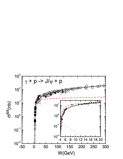
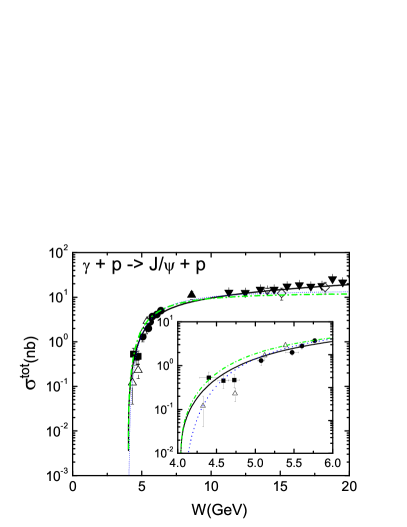
Figure 3: The total cross section of the $\gamma+p\to J/\psi+p$ reaction as function of the $\gamma p$ invariant mass $W$. Left: the black solid and red dashed are the results from using ($\alpha_{0}=1.25$, $\beta_{c}=0.84$ GeV^-1; called the PM model) and ($\alpha_{0}=1.08$, $\beta_{c}=1.21$ GeV^-1) within the model which include both the $\pi$-exchange and Pomeron-exchange mechanisms. The magenta dotted curve in the insert is the contribution from the $\pi$ exchange. Right: the black solid, blue dotted and green dot-dashed lines are from the PM model, the $2g$ model of Ref.brodsky-2 , and the $2g+3g$ model based on Eq.(35). The experimental data are from Barate:1986fq ; Binkley:1981kv ; Camerini:1975cy ; Denby:1983az ; Frabetti:1993ux ; Gittelman:1975ix ; Anderson ; H1 ; ZEUS .

We next consider the model of Ref.brodsky-2 based on the two-gluon ($2g$) and three-gluon ($3g$) exchange mechanisms. In terms of the normalization defined by Eq.(2), the amplitude of this model can be written as

$$<\vec{k}\lambda_{J/\psi}m^{\prime}_{s}|t(W)|\vec{q}\lambda_{\gamma}m_{s}> = \frac{1}{(2\pi)^{3}}\frac{1}{\sqrt{2E_{J/\psi}(k)}}\sqrt{\frac{m_{N}}{E_{N}(k)}}\sqrt{\frac{m_{N}}{E_{N}(q)}}\frac{1}{\sqrt{2q}}$$ (35)

$$\times\frac{4\sqrt{\pi}}{\sqrt{6}}\frac{qw}{m_{N}}[\textbf{M}_{2g}+\textbf{M}_{3g}]$$

with

$$\textbf{M}_{2g} = \frac{A_{2g}}{4\sqrt{\pi}}\frac{1-x}{Rm_{J/\psi}}e^{bt/2}\,,$$ (36)

$$\textbf{M}_{3g} = \frac{A_{3g}}{4\sqrt{\pi}}\frac{1}{R^{2}m^{2}_{J/\psi}}e^{bt/2}\,,$$ (37)

$$x = \frac{2m_{N}m_{J/\psi}+m^{2}_{J/\psi}}{W^{2}-m^{2}_{p}}\,.$$ (38)

where $R=1$ fm, $b=1.13$ GeV^-2 are taken from Ref. brodsky-2 . We follow Ref.brodsky-2 to determine the parameters $A_{2g}$ and $A_{3g}$ by fitting the data up to only 20 GeV. In the two-gluon-exchange model ($2g$), we set $A_{3g}=0$ and obtain $A_{2g}=0.028$ MeV^-2 from the fit. In the $2g+3g$ model, the fit is obtained by choosing $A_{2g}=0.023$ MeV^-2 and $A_{3g}=2000$ MeV^-2. The fits for the $2g$ and $2g+3g$ models are the dotted and dot-dashed curves in the right-hand side of Fig.3, respectively. Clearly, they have differences with that (black solid) of the PM model, as can be seen more clearly in the insert in the right-hand side of Fig.3. Here we also see that the data in the region near the $J/\Psi$ production threshold are very limited and uncertain. We will therefore perform calculations using the PM, $2g$, and $2g+3g$ models to examine the model dependence of our predictions. Clearly, precise data in the near threshold region are needed to make progress.

IV.2 Photo-production of $J/\Psi$-Nucleus bound states

Following the previous investigations brodsky90 ; gao01 , we assume that the interaction between a $J/\Psi$ and a nucleus with mass number $A$ can be parameterized as a non-relativistic potential of the following Yukawa form

$$V_{J/\Psi,A}(r)=-\alpha_{A}\frac{e^{-\mu_{A}r}}{r}\,.$$ (39)

There exists two different approaches to determine the parameters $\alpha_{A}$ and $\mu_{A}$ for the nucleon with $A=1$. We will explain these in the following two subsections.

IV.2.1 Pomeron-quark coupling model

Motivated by the previous studies in Quantum Electrodynamics, it is assumed in the approach of Ref.brodsky90 that the $J/\Psi$-A forward angle scattering amplitude at very high energy can be related to the matrix element of the potential Eq.(39) which is understood to be valid only in the region where $J/\Psi$ moves non-relativistically. They further assume that the $J/\Psi$-A amplitudes can be calculated by using the Pomeron-exchange model of Dannachie and Landshoffdonn84 . In the very high energy approximation, the differential cross section of $J/\Psi$-A elastic scattering can be related to the parameters $\alpha_{A}$ and $\mu_{A}$ of the potential Eq.(39) by following relation

$$\frac{d\sigma}{dt}(J/\Psi\,A\rightarrow J/\Psi\,A) = \frac{[2\beta_{c}F_{J/\Psi}(t)]^{2}[3A\beta_{u/d}F_{A}(t)]^{2}}{4\pi}$$ (40)

$$= \frac{4\pi\alpha^{2}_{A}}{(-t+\mu^{2}_{A})^{2}}\,,$$ (41)

where $t$ is the momentum-transfer squared, $\beta_{u/d}$ ($\beta_{c}$) is the Pomeron coupling with the $up/down$ ( $charmed$ ) quarks, $F_{J/\Psi}(t)$ and $F_{A}(t)$ are the form factors for $J/\Psi$ and the nucleus with mass number $A$, respectively. They further assume that in the $t\rightarrow 0$ limit, the slope of ${d\sigma}/{dt}$ is mainly determined by $dF_{A}(t)/dt$ and that $F_{A}(t)$ can be identified with the nuclear electromagnetic form factor. One then gets the following relations

$$\mu^{-2}_{A} = |\frac{dF_{A}(t)}{dt}|_{t=0}=\frac{<R^{2}_{A}>}{6}\,,$$ (42)

$$\alpha_{A} = \frac{[2\beta_{c}][3A\beta_{u/d}]}{4\pi}\mu^{2}_{A}\,.$$ (43)

The radius $<R^{2}_{A}>^{1/2}$ can be taken from Ref.nucl-data . The Pomeron-quark coupling constants can be taken from fits to the data of meson-nucleon scattering or photo-production of vector mesons. Once $\alpha_{A}$ and $\mu_{A}$ of the potential Eq.(39) are determined, we can predict the possible $J/\Psi$-nucleus bound states. In Table 1, we list our results for proton ($A=1)$, ${}^{3}He$ (A=3) and ${}^{12}C$ (A=12) for various sets of Pomeron-quark coupling constants. The first rows in the results for each $A$ are based on the flavor independent $\beta_{u/d}=\beta_{c}=1.85$ GeV^-1 of Ref.brodsky90 . The other two results use the Pomeron-quark coupling constants $\beta_{u/d}=2.05$ GeV^-1 determinedOL02 in the fits to the data of photo-production of $\rho$ and $\omega$, and $\beta_{c}$ determined from the fits described in section IV.A.

Table 1: Parameters for determining the potential Eq.(39) using the Pomeron-quark coupling model defined by Eqs.(41)-(43). The predicted binding energies (B.E.) for proton ($A=1)$, ${}^{3}He$ (A=3) and ${}^{12}C$ (A=12) are also listed.

A	$<R^{2}_{A}>^{1/2}$	$\mu_{A}$	$\beta_{u/d}$	$\beta_{c}$	$\alpha_{A}$	B.E.
	(GeV-1)	(GeV)	(GeV-1)	(GeV-1)		(MeV)
1	3.9	0.63	1.85	1.85	0.64	-
			2.05	1.21	0.47	-
			2.05	0.84	0.33	-
3	9.5	0.26	1.85	1.85	0.33	19.86
			2.05	1.21	0.23	3.27
			2.05	0.84	0.16	0.04
12	12.69	0.19	1.85	1.85	0.73	280.0
			2.05	1.21	0.53	165.0
			2.05	0.84	0.37	67.0

With the determined potential parameters $\alpha_{A}$ and $\mu_{A}$, the predicted binding energies ($B.E.$) for each considered nuclear system are listed in the last column of Table 1. For the $A=1$ case, we see that there is no $J/\Psi$-$N$ bound state. But all three models predict bound $[^{3}He]_{J/\Psi}$ and $[^{12}C]_{J/\Psi}$ states. In the left-hand side of Fig.4, we show the predicted cross sections of $\gamma+^{4}He\to[^{3}He]_{J/\Psi}+n$. Clearly, the predicted cross sections depend on the Pomeron-quark coupling constants. Furthermore, their magnitudes depend sensitively on the binding energy (B.E.) of the predicted $[^{3}He]_{J/\Psi}$ system. As the binding energy decreases from 19.86 MeV to 0.04 MeV, the predicted cross sections drop by two orders in magnitude. This can be understood from the right-hand side of Fig.4 where we compare the $J/\Psi$-${}^{3}He$ relative wavefunctions which are used in predicting the cross sections in the left-hand side. We see that the wavefunction (solid black) for B.E. $=19.86$ MeV is much shorter range than the other two cases and hence gives more cross sections in this large momentum-transfer reaction. This is explicitly illustrated in Fig.5 where we show that the cross section (red dashed curve) calculated from keeping only the high momentum part ($p_{J/\psi}>1400$ MeV) of the $J/\Psi$ wavefnction in the integration in Eq.(32) is very close to the full calculation (solid black curve).

In Fig.6, we see that the predicted differential cross sections are forward peaked, as expected from the Pomeron-exchange mechanism. In Fig.7, we show that the predicted cross sections depend on the $\gamma+N\rightarrow J/\Psi+N$ model. Their maximum values are, however, comparable $\sim 0.1-0.3$ pico-barn. Clearly, it is important to get accurate data of $\gamma+N\rightarrow J/\Psi+N$ at low energies to refine the employed model for making more precise predictions.

The $[^{12}C]_{J/\Psi}$ can be produced by $\gamma+^{13}C\rightarrow[^{12}C]_{J/\Psi}+n$. However, making predictions for the cross sections of this process is beyond the scope of this paper since the simple s-wave description of the nuclei in section III is no longer a reasonable approximation for nuclei heavier than ${}^{4}He$.

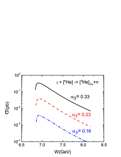
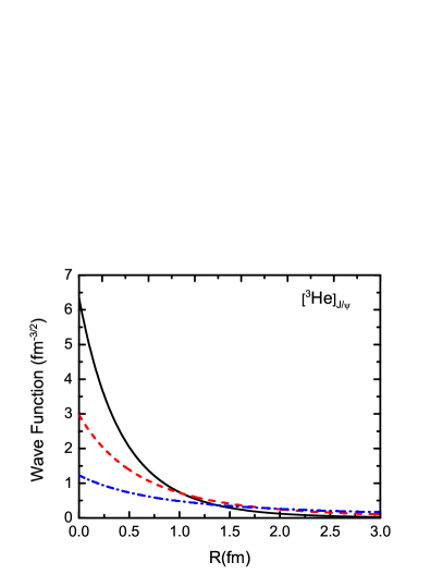
Figure 4: The total cross section of $\gamma+[^{4}He]\to^{3}He_{[J/\psi]}+n$ as function of $\gamma$-${}^{4}He$ invariant mass $W$ (left) and the wave function (right) for $J/\psi-^{3}He$ system. The black solid, red dashed and blue dotted-dashed lines are calculated by using the potential Eq.(39) with $A=3$, $\mu_{A}=0.257$ GeV and $\alpha_{A}=0.33,0.23,0.16$, respectively.

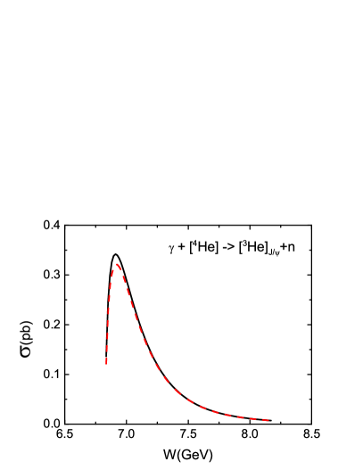
Figure 5: The cross section of $\gamma+[^{4}He]\to[^{3}He]_{[J/\psi]}+n$ as function of $\gamma$-${}^{4}He$ invariant mass $W$. The red dashed curve is obtained from keeping only the contribution from the $J/\Psi$ wavefunction with $k>1400$ MeV in the integration of Eq.(32).

Figure 6: The differential cross section of $\gamma+[^{4}He]\to[^{3}He]_{[J/\psi]}+n$ vs the angle of out going $N$ with the center mass $6.9$ GeV.

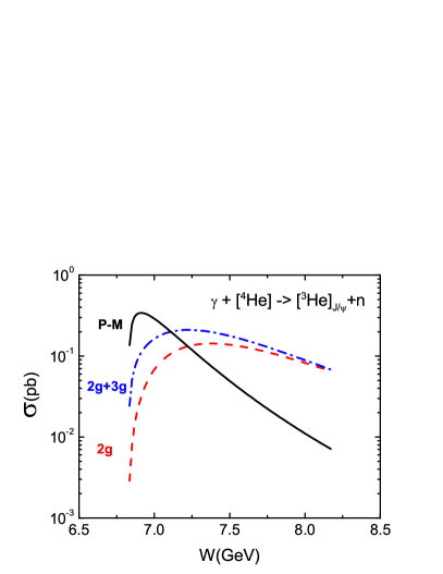
Figure 7: The total cross section of $\gamma+[^{4}He]\to[^{3}He]_{[J/\psi]}+n$ vs the certain mass of system. The black solid, red dashed and blue dot-dashed lines are for the pomeron and $\pi$ exchange, Brodsky’s 2g model and 2g+3g model, respectively.

IV.2.2 Folding model

While all three $J/\Psi$-$N$ models listed in Table 1 do not have bound states, there exist a possibility that adding the $J/\Psi$-$N$ interactions from the nucleons in a nucleus could lead to bound states. To explore this possibility, we follow the usual nuclear physics approach to construct a folding potential for the interaction between a $J/\Psi$ and a nuclear system,

$$V_{J/\Psi,A}(r)=\int v_{J/\Psi,N}(\vec{r}-\vec{r}^{\,\,{}^{\prime}})\rho_{A}(\vec{r}^{\,\,{}^{\prime}})d\vec{r}^{\,\,{}^{\prime}}\,,$$ (44)

where $v_{J/\Psi,N}(r)=V_{J/\Psi,1}(r)$ as defined by Eq.(39) with $A=1$, and the nuclear density is normalized by

$$\int\rho_{A}(\vec{r}^{\,\,{}^{\prime}})d\vec{r}^{\,\,{}^{\prime}}=A\,.$$ (45)

For ${}^{3}He$ we use $\rho_{A}(\vec{r})=\rho_{0}e^{-r^{2}/b^{2}}$ with $b=1.32$ fm which is obtained by fitting the ${}^{3}He$ charge form factor at low momentum-transfer. For heavy nuclei, we use the Woods-Saxon formbohr-moltt

$$\rho_{A}(\vec{r})=\rho_{0}\frac{1}{1+e^{(r-R)/t}}$$ (46)

with $R=1.1A^{-1/3}$ fm and $t=0.53$ fm.

Our results using the parameters of Ref.brodsky90 to calculate $v_{J/\Psi,N}(\vec{R})$ in Eq.(44) are listed in the first row of Table 2. We see that the folding model gives $1.62$ MeV ($7.0$ MeV) for $[^{3}He]_{J/\Psi}$ ( $[^{12}C]_{J/\Psi}$) which are much less than $19.86$ MeV ( $280$ MeV) listed in Table 1. The predicted cross sections for $\gamma+^{4}He\rightarrow[^{3}He]_{J/\Psi}+n$ are also found to be much weaker, close to the blue dot-dashed curve ($\alpha_{3}=0.16$) in Fig.4. Clearly, it is difficult to measure such a loosely bound $[^{3}He]_{J/\Psi}$ state.

To examine the model dependence, we also consider folding potentials by using three other $J/\Psi$-$N$ models. Twobrodsky-1 ; russia of them are constructed by using the results from the heavy quark effective field theory calculation by Peskinpesk79 . The third onelqcd is from Lattice QCD calculation. Their results can also be written in the Yukawa form of Eq.(39) with $A=1$. We find that these three models do not generate a $[^{3}He]_{J/\Psi}$ bound state as indicated in Table 2. For ${}^{12}C$, the binding energies from folding model are much weaker than those listed in Table 1 from the Pomeron-quark coupling model.

Table 2: The binding energy of $J/\psi$-nucleus calculated with the folding potential defined by Eq.(44) with parameters of $v_{J/\Psi,N}=-\alpha_{1}\frac{e^{-\mu_{1}r}}{r}$ taken from different references. The parameters of Ref.brodsky-1 are obtained from reproducing the scattering length $a=-0.24$ fm given in Ref.brodsky-1 . (A Gaussian form of the $v_{J/\Psi,N}$ was used in Ref.brodsky-1 )

Model	Parameter(MeV)		Binding Energy(MeV)
	$\alpha_{1}$	$\mu_{1}$ (GeV)	$[H]_{J/\Psi}$	$[^{3}He]_{J/\Psi}$	$[^{12}C]_{J/\Psi}$
Ref.brodsky90	0.64	0.63	-	1.62	7.0
Ref.brodsky-1	0.20	0.63	-	-	0.91
Ref.lqcd	0.10	0.63	-	-	0.003
Ref.russia	0.06	0.63	-	-	-

IV.3 Photo-production $J/\Psi$-$(q^{6})$ bound states

In Ref.brodsky-2 , it was suggested that a $c\bar{c}$ system could interact strongly with the color octet 3-quark $[\bar{q}^{3}]_{8}$ component of the six-quark cluster ($[q^{6}]=[q^{3}]_{8}[\bar{q}^{3}]_{8}$) which could dominant the short-range part of the deuteron wavefunction. The possible attractive force between a $J/\Psi$ and a six-quark cluster was suggested in the study of Ref.brodsky-3 where the excitation of a hidden charm $|qqqqqqc\bar{c}>$ state is introduced to explain the spin correlation of $pp$ elastic scattering near the $J/\Psi$ production threshold. Here we examine the condition under which a bound $[q^{6}]_{J/\Psi}$ color singlet state can be produced in the $\gamma+^{3}He\rightarrow[q^{6}]_{J/\Psi}+N$ reaction. Unlike the predictions for the photo-production of $[^{3}He]_{J/\Psi}$ described in the previous subsection, very little information on $[q^{6}]$ and the $[q^{6}]-{J/\Psi}$ interaction is available. We thus need to make various assumptions which can only be considered to be plausible for estimating the production cross sections.

In the impulse approximation, as described in section II, we need the initial $N$-$[q^{6}]$ wavefunction in ${}^{3}He$ and the final $J/\Psi$-$[q^{6}]$ wavefunction to calculate the cross section of $\gamma+^{3}He\rightarrow[q^{6}]_{J/\Psi}+N$. In the following subsections, we explain our procedure for modeling these two ingredients of our predictions.

IV.3.1 Wavefunction of $N$-$q^{6}$ in ${}^{3}He$

We start with a formulation of Refs.fasano-1 ; lee-matsuyama within which the Hamiltonian for a two nucleon system is written as

$$H=H_{0}+v_{NN}+\sum_{\alpha}h_{[q^{6}]^{\alpha}\leftrightarrow NN}\,,$$ (47)

where $\alpha$ denotes collectively the total angular momentum $J$, the total isospin $T$, and the parity $P$, and $v_{NN}$ is a meson-exchange nucleon-nucleon ($NN$) interaction. The vertex interaction $h_{[q^{6}]^{\alpha}\leftrightarrow NN}$ defines the formation of a six-quark state $[q^{6}]^{\alpha}$ in $NN$ collisions. The six-quark states $[q^{6}]^{\alpha}$ are identified with the states predicted by the Bag model calculations of Muldermulder . By appropriately choosing the form of the vertex interaction $h_{[q^{6}]^{\alpha}\leftrightarrow NN}$, the NN scattering amplitudes derived from the Hamiltonian Eq.(47) are identical to those given by using the P-matrix approach of Jaffe and Lowlow and the Compound Bag Model formulation developed in Refs.itep ; bakker .

We will make use of the results of Fasano and Leefasano-1 ; fasano-2 . They determined the mass $M_{\alpha}$ of $[q^{6}]^{\alpha}$ cluster and the interaction $h_{[q^{6}]^{\alpha}\leftrightarrow NN}$ for $\alpha=^{1}S_{0}$ and ${}^{3}S_{1}$ by fitting the $NN$ scattering phase shifts up to 1 GeV. Within the simple s-wave harmonic oscillator model for ${}^{3}He$, the probabilities $P_{[q^{6}]^{\alpha}}$ of finding the $[q^{6}]^{\alpha}$-$N$ in ${}^{3}He$ are estimatedfasano-2 to be $P_{[q^{6}]^{{}^{1}S_{0}}}=0.7\%$ and $P_{[q^{6}]^{{}^{3}S_{1}}}=0.06\%$. For simplicity, we neglect the small ${}^{3}S_{1}$ component. The bare mass of $[q^{6}]$ determined in Ref.fasano-1 is $M_{{}^{1}S_{0}}=2150$ MeV. Here we will use these information to model the relative wavefunction of $[q^{6}]^{\alpha}$-$N$ which is needed to calculate the cross sections of $\gamma+^{3}He\rightarrow[q^{6}]_{J/\Psi}+N$.

Figure 8: The solid curve is the normalized density distribution calculated from using Eqs.(50)-(51) with $b=1.35$ fm and $l_{c}=0.5$ fm. The dashed line defines $r_{c}=0.29$ fm for obtaining the probability $P_{[q^{6}]^{{}^{1}S_{0}}}=0.7\%$ for finding the $[q^{6}]-N$ component in ${}^{3}He$ by using Eq.(53).

We assume that the charge distribution in the region with the distance $r\leq r_{c}$ from the center of ${}^{3}He$ is completely due to $[q^{6}]^{\alpha}$-$N$ components of the wavefunction. This is illustrated in Fig.8. Each $r_{c}$ clearly corresponds to a choice of $P_{q^{6}}$. Within such a model, the charge form factor of ${}^{3}He$ is written as

$$F_{c}(Q^{2})=F_{c}^{N^{3}}(Q^{2})+F_{c}^{q^{6}-N}(Q^{2}).$$ (48)

We next observe that within the conventional nuclear modelschiavilla , the impulse approximation (IA) calculation, which includes only the one-body nucleon current, of $F_{c}(Q^{2})$ is very close to the data in $Q^{2}\leq$ about 10 fm^-2 and can be reproduced very well by the Gaussian distribution of the s-wave harmonic oscillator wavefunction. The IA results from Ref.schiavilla in this $Q^{2}$ region are the solid squares in Fig.9. We next demand that the s-wave three-nucleon wavefunction reproduce these IA results. In addition, the resulting $F_{c}(Q^{2})$ in the higher $Q^{2}$ region must have the similar structure of IA up $Q^{2}\sim 20$ fm^-2 although we do not have higher partial wave components of the three-nucleon wavefunction. We achieve this by using the s-wave harmonic oscillator wavefunction with Jastrow two-body correlation used in Refs.feshbach ; lee . We write

$$F_{c}(Q^{2}) = \int e^{-i\vec{Q}\cdot\vec{r}}\rho(\vec{r})d\vec{r}$$ (49)

with

$$\rho(\vec{r}_{1})=\int d\vec{r}_{2}\rho_{2}(\vec{r}_{1},\vec{r}_{2})\,,$$ (50)

where the two-body density is defined by

$$\rho_{2}(\vec{r}_{1},\vec{r}_{2}) = Ne^{-\frac{r^{2}_{1}+r^{2}_{2}}{2b^{2}}}(1-e^{-\frac{|\vec{r}_{1}-\vec{r}_{2}|^{2}}{2l_{c}^{2}}})\,,$$

$$N = \frac{1}{(\sqrt{\pi}b)^{3}}\sqrt{\frac{[l_{c}^{2}+b^{2}]^{3/2}}{[l_{c}^{2}+b^{2}]^{3/2}-l_{c}^{3}}}\,.$$ (51)

As seen in Fig.9, the solid black curve calculated with $b=1.35$ fm and $l_{c}=0.5$ fm can reproduce the impulse approximation calculation results (solid squares) given in Ref.schiavilla up to $Q^{2}\sim 10$ fm^-2. At higher $Q^{2}$, the solid curves have the similar structure of the IA results. For our present s-wave calculations, we consider the solid curves in Fig.9 as the $F_{c}(Q^{2})$ in Eq.(48). Accordingly, the $NNN$ contribution in Eq.(48) is calculated from

$$F_{c}^{N^{3}}(Q^{2})=\int^{\infty}_{r_{c}}r^{2}dr\int d\Omega_{r}e^{-i\vec{Q}\cdot\vec{r}}\rho(\vec{r})\,$$ (52)

and the probability $P_{[q^{6}]}$ is defined by

$$P_{q^{6}} = \int^{r_{c}}_{0}r^{2}d{r}\int d\Omega_{r}\rho(\vec{r})\,.$$ (53)

For $P_{q^{6}}=0.7\%$ determined in Ref.fasano-1 within the Compound Bag Model of NN scattering, we choose $r_{c}=0.292$ fm to calculate Eq.(52) and get the blue dotted curve in the left-hand side of Fig.9. In the right-hand side, the blue dotted curve is from the calculation using Eq.(52) with $r_{c}=0.630$ fm which gives $P_{q^{6}}=6.3\%$. Clearly, both results agrees well with the IA (solid squares) and the solid curve only in the low $Q^{2}$ region. Our next task is to model $F^{q^{6}-N}(Q^{2})$ such that for each $r_{c}$, $F_{c}(Q^{2})$ (solid black curve) in Fig.9 up to $Q^{2}\sim 15$ fm² can be reproduced, as required by Eq.(48).

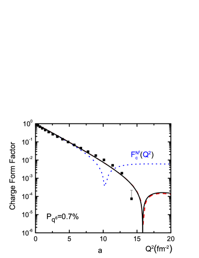
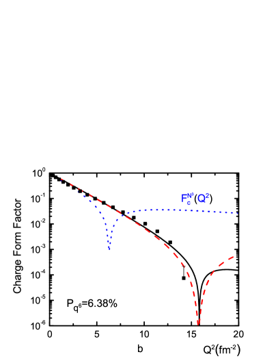
Figure 9: The charge form factor $F_{c}(Q^{2})$ for ${}^{3}He$. The solid squares are from the Impulse Approximation (IA) calculation of Ref.schiavilla . The dotted blue curves are $F^{N^{3}}_{c}(Q^{2})$ calculated from using Eq.(52) with $r_{c}=0.292$ fm and $P_{q^{6}}=0.7\%$ (left) and $r_{c}=0.630$ fm and $P_{q^{6}}=6.3\%$ (right). The red dashed curves are from adding the $q^{6}-N$ contributions calculated from using Eq.(54) with $b^{*}=0.185$ fm (left) and $b^{*}=0.414$ fm (right).

For simplicity, we assume that $F_{c}^{q^{6}-N}(Q^{2})$ can be calculated from a normalized Gaussian distribution

$$F_{c}^{q^{6}-N}(Q) =P_{q^{6}} \int e^{-i\vec{Q}\cdot\vec{r}}[\frac{1}{(\sqrt{\pi}b^{*})^{3}}e^{\frac{-r^{2}}{b^{*2}}}]d\vec{r}\,.$$ (54)

Accordingly, the mean radius of $q^{6}$-$N$ can be defined by

$$<r^{2}>=\int[\frac{1}{(\sqrt{\pi}b^{*})^{3}}e^{\frac{-r^{2}}{b^{*2}}}]r^{2}d\vec{r}\,.$$ (55)

We adjust $b^{*}$ for each $P_{q^{6}}$ to fit the solid curves in Fig.9. We find that if $P_{q^{6}}$ is larger than $6.5\%$, no $b^{*}$ can fit the form factor defined by Eq.(48) in the $Q^{2}<20$ fm^-2 region. In the cluster model of Ref.japan-he3 , $P_{q^{6}}=4.0\%$ is obtained from fitting the ${}^{3}He$ form factor. The $P_{q^{6}}=15\%$ determined in Ref.vary by fitting the structure function of ${}^{3}He(e,e^{\prime})$ is beyond what our formulation can accommodate. For comparison, we thus choose three different models with $P_{q^{6}}=0.7\%,4\%$, and $6.38\%$ for our calculations. In Table 3, we list $r_{c}$, $b^{*}$, and also $<r^{2}>^{1/2}$ calculated from using Eq.(55) for these three cases. Our fits are the red dashed curves in Fig.9 for $P_{q^{6}}=0.7\%$ (left) and $6.38\%$ (right).

Once $b^{*}$ is determined, we then assume that the relative wavefunction of $[q^{6}]$-N can be described by the harmonic wavefunction with the same $b^{*}$. This should be reasonable for making order of magnitude estimates in this work. A more sophisticated approach should account for the quark charge distribution in $[q^{6}]$ which is beyond the scope of this work. Also, the sharp cutoff at $r=r_{c}$ to define $F_{c}^{N^{3}}$ in Eq.(52) should perhaps be better modeled. For our present qualitative estimations, this simple procedure should be sufficient.

Table 3: The parameters for ${}^{6}q$-$N$ and ${}^{6}q$-$J/\psi$ systems. See text for the explanations of the notations.

	$q^{6}$-$N$				$q^{6}$-$J/\psi$
Model	$P_{q^{6}}$	$r_{c}$	$b^{*}$	${<r^{2}>^{1/2}}$	$\mu_{q^{6}}$	$\alpha_{q^{6}}$	B.E.
		(fm)	(fm)	(fm)	(GeV)		(MeV)
$A_{1}$	0.7%	0.292	0.185	0.226	0.6	1.33	498.42
$A_{2}$					1.0	1.50	389.63
$B_{1}$	4.0%	0.533	0.346	0.424	0.6	0.83	104.08
$B_{2}$					1.0	1.05	79.77
$C_{1}$	6.38%	0.630	0.414	0.507	0.6	0.75	65.84
$C_{2}$					1.0	0.97	51.33

IV.3.2 Wavefunction of ${}^{6}q$-$J/\psi$ bound state

We follow the procedure of subsection IV.B to assume that the $q^{6}$-$J/\Psi$ bound states ($[q^{6}]_{J/\Psi}$) are also defined by a potential, of Yukawa form

$$V_{J/\Psi,q^{6}}(r) = -\alpha_{q^{6}}\frac{e^{-\mu_{q^{6}}r}}{r}\,.$$ (56)

We expect that if a $[q^{6}]_{J/\Psi}$ bound state can be produced, its size must be small for color field to give strong attractive force. Thus it is reasonable to assume that the mean radius of $[q^{6}]_{J/\Psi}$ is close to the value $<r^{2}>^{1/2}$ of the initial $q^{6}$-$N$ system listed in Table 3. We find that such a small size can be generated from choosing $\mu_{q^{6}}>0.6$ GeV in defining the potential Eq.(56). Once a value of $\mu_{q^{6}}$ is chosen, we then determine the potential strength $\alpha_{q^{6}}$ by requiring

$$<r^{2}>=\int|\phi_{q^{6},J/\Psi}(\vec{r})|^{2}r^{2}d\vec{r}\,,$$ (57)

where $\phi_{q^{6},J/\Psi}(\vec{r})$ is the $J/\Psi$-$q^{6}$ relative wavefunction generated from the potential Eq.(56), and the values of $<r^{2}>^{1/2}$ for various considered cases are listed in Table 3. The resulting $\alpha_{q^{6}}$ and the binding energies (B.E.) are also listed there. Here we note that the binding energy increases as the mean radius $<r^{2}>^{1/2}$ and the corresponding probability $P_{q^{6}}$ decrease.

IV.3.3 The Results of $\gamma+^{3}He\to[q^{6}]_{J/\psi}+N$

With the wavefunctions for $q^{6}$-$N$ and $q^{6}$-$J/\Psi$ specified in the previous subsections, we can use the formula in section III, with trivial changes in notations and spin quantum numbers, to calculate the total cross section of $\gamma+^{3}He\to[q^{6}]_{J/\psi}+N$. However, we need to multiply the results by the probability $P_{q^{6}}$ of the $N$-$[q^{6}]$ component in ${}^{3}He$; namely the results from using Eq.(19) is changed to

$$\frac{d\sigma}{d\Omega}\rightarrow P_{[}q^{6}]\times[\frac{d\sigma}{d\Omega}]_{0}\,,$$ (58)

where $[\frac{d\sigma}{d\Omega}]_{0}$ is calculated from using Eq.(19) and all subsequent equations in section III.A.

We first consider the case that $P_{[q^{6}]}=0.7\%$ as determined in Refs.fasano-1 ; fasano-2 from fitting the $NN$ phase shifts up to 1 GeV. By using the parameters for models $A_{1}$ and $A_{2}$ listed in Table 3, we obtain the results shown in Fig.10. We observe that with the same small radius $<r^{2}>^{1/2}=0.226$ fm for the produced $[q^{6}]_{J/\psi}$ system, the predicted cross sections are very close despite their potential range, measured by $1/\mu_{q^{6}}$, and coupling constant $\alpha_{q^{6}}$ can be very different. The same finding is also from comparing the predicted cross sections from the models $B_{1}$ and $B_{2}$, and also the models $C_{1}$ and $C_{2}$.

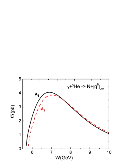
Figure 10: The total cross section of $\gamma+^{3}He\to[q^{6}]_{J/\psi}+N$ as function of the $\gamma$-${}^{3}He$ invariant mass $W$. The black solid and red dashed curves are for the case $A_{1}$ and $A_{2}$ in the Table 3, respectively.

In the left-hand side of Fig.11, we show the dependence of the predicted cross sections on $P_{q^{6}}$ by comparing the cross sections from three models $A_{1}$, $B_{1}$, and $C_{1}$ listed in Table 3. We observe that as $P_{q^{6}}$ decreases, the peak is shifted to higher energies. Each case has different threshold energy due to their differences in binding energies, as seen in Table 3. Their magnitudes are comparable despite their $P_{q^{6}}$ are very different. We find that this is due to the fact that the cross section $[\frac{d\sigma}{d\Omega}]_{0}$ in Eq.(58) for the model with smaller $P_{q^{6}}=0.7\%$ is a factor of about 10 larger than that for the model with larger $P_{q^{6}}=6.38\%$, since this large momentum transfer reaction favors the production of $[q^{6}]_{J/\Psi}$ with smaller size characterized by $<r^{2}>^{1/2}$ in Table 3. The situation is similar to what we discussed in explaining the results shown in Fig.4. Thus the magnitudes of the cross sections from three models at peak positions are comparable because the factor of about 10 difference in $[\frac{d\sigma}{d\Omega}]_{0}$ in Eq.(58) is compensated by the similar factor of about 10 in $P_{q^{6}}$. However, the three models have rather different energy dependence, as also seen in the left-hand side of Fig.11. On the other hand, they are all forward peaked, as shown in the right-hand side of Fig.11 for the differential cross sections at $W=6.6$ GeV.

The results shown in Fig.11 suggest that the upper bound of the predicted total cross sections of $\gamma+^{3}He\rightarrow[q^{6}]_{J/\Psi}+N$ is about 2 - 4 pico-barn

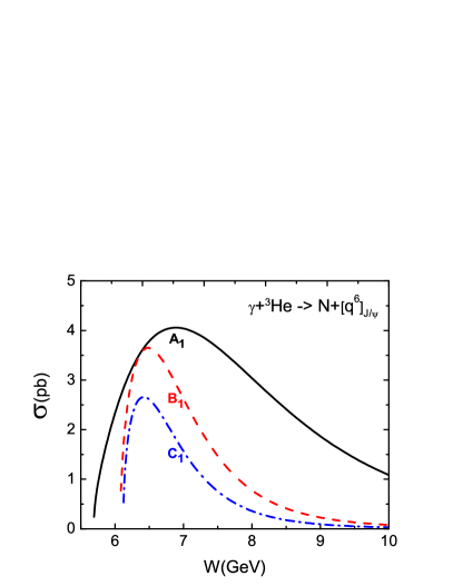
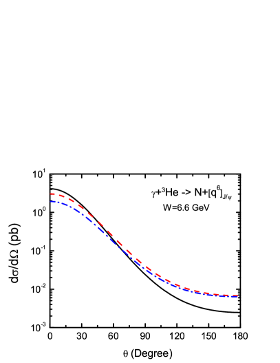
Figure 11: The black solid, red dashed and blue dotted-dashed lines are from Models $A_{1}$, $B_{1}$, and $C_{1}$ of Table 3, respectively. Left: The total cross section of $\gamma+^{3}He\to[q^{6}]_{J/\psi}+N$ as function of the $\gamma$-${}^{3}He$ invariant mass $W$. Right:The differential cross section of $\gamma+^{3}He\to q^{6}_{[J/\psi]}+N$ of the outgoing $N$ at $\gamma$-${}^{3}He$ invariant mass $W=6.6$ GeV.

V summary and discussions

We have presented predictions of the cross sections of $\gamma+^{4}He\rightarrow N+[^{3}He]_{J/\Psi}$ reaction at energies near the $J/\Psi$ production threshold. In the impulse approximation, the calculations have been performed by using several $\gamma+N\rightarrow J/\Psi+N$ models based on the Pomeron-exchange and pion-exchange mechanisms. The $J/\Psi$ wavefunctions in $[^{3}He]_{J/\Psi}$ are generated from various $J/\Psi$-nucleus potentials which are constructed by either using a procedure based on the Pomeron-quark coupling mechanismbrodsky90 , or folding a $J/\Psi$-N potential $v_{J/\Psi,N}$ into the nuclear densities. We consider $v_{J/\Psi,N}$ derived from the effective field theory approach, Lattice QCD, and Pomeron-quark coupling model. The upper bound of the predicted total cross sections is about 0.1 - 0.3 pico-barn.

Clearly, our investigations are only for estimating the cross sections to facilitate the experimental considerations of possible measurements of $[^{3}He]_{J/\Psi}$ bound states at Jefferson Laboratory. Several improvements are needed for more quantitative predictions. First we need precise data of $\gamma+p\rightarrow J/\Psi+p$ near threshold to distinguish several models we have considered and also to develop a more sophisticated model.We also need the data to pin down the $J/\Psi$-N interaction for a more realistic calculation of $J/\Psi$-nucleus potential such as the folding model considered in this work. One possibility is to use the $\pi+^{2}H\rightarrow p+J/\Psi+n$ reaction to extract the $J/\Psi$-$N$ scattering length, as suggested in Ref.brodsky-1 . Alternatively, we can apply the model presented in this paper to determine the $J/\Psi$-$N$ interactions by investigating the $\gamma+^{2}H\rightarrow p+J/\Psi+n$ reaction. Possible experiments on these two processes will be very useful. We of course also need to use more realistic wavefunctions for ${}^{3}He$ and ${}^{4}He$ while the s-wave oscillator wavefunctions employed in this investigation are reasonably consistent with the charge form factors calculated from the conventional nuclear models.

Motivated by the previous investigationsbrodsky-3 ; brodsky-2 on the effects due to multi-quark clusters in $pp$ and $\gamma+^{2}H\rightarrow J/\Psi+n+p$, we have also considered the possibility of the production of a $[q^{6}]-J/\Psi$ bound state due to a six-quark $[q^{6}]$ cluster in ${}^{3}He$. The Compound Bag Model of $NN$ scattering and the quark cluster model of nuclei are used to estimate the $[q^{6}]$-N wavefunction in ${}^{3}He$ by imposing the condition that the sum of the contributions from $[q^{6}]$-N and $NNN$ components to the ${}^{3}He$ charge form factor must be consistent with what are predicted by the conventional nuclear modelsschiavilla which explain the data very well. The upper bound of the predicted total cross sections of $\gamma+^{3}He\rightarrow[q^{6}]_{J/\Psi}+N$ is about 2 - 4 pico-barn, depending on the model of $\gamma+N\rightarrow J/\Psi+N$ used in the calculations. If such bound states can be identified, it will open up a new window for investigating the role of the gluon field in determining the hadron structure.

- (1) M.E. Peskin, Nucl. Phys. B156, 365 (1979)
- (2) G. Bhanot and M.E. Peskin, Nucl. Phys. B156, 391 (1979)
- (3) M. Luke, A.V. Manohar, and M.J. Savage Phys. Lett B 288, 355 (1992)
- (4) S. J. Brodsky and G. A. Miller, Phys. Lett. B 412, 125 (1997).
- (5) Taichi Kawanai and Shoichi Sasaki, Phys. Rev. D 82, 091501 (2010)
- (6) A.B. Kaidalov and P.E. Volkovitsky, Phys. Rev. Lett 69, 3155 (1992)
- (7) S.J. Brodsky, I.A. Schmidt, and G.F. Teramond, Phys. Rev. Lett. 64, 1011 (1990)
- (8) A. Donnachie and P.V. Landshoff, Nucl. Phys. B244, 322 (1984)
- (9) Herman Feshbach, Theoretical Nuclear Physics, Nuclear Reactions (Wiley, New York, 1992)
- (10) Z.-E. Meziani, K. Hafidi, X. Uian, and N. Sparveris et al., Proposal ”Near Threshold Electroproduction of at 11 GeV”, PR12-12-006(2012), PAC39, Jefferson Laboratory (2012)
- (11) S. J. Brodsky and G.F. de Teramond, Phys. Rev. Lett 60, 1924 (1988)
- (12) S. J. Brodsky, E. Chudakov, P. Hoyer, and J.M. Laget, Phys. Lett B498, 23 (2001)
- (13) R.L. Jaffe and F. Low, Phys. Rev. D 19, 2105 (1979); F. Low in Pointlike Structure Inside and Outside Hadrons, Proceedings of 1979 Erice Summer School, Editted by A. ZiChiChi (Plenum, New York, 1979), p. 155.
- (14) P. J. Mulders. Phys. Rev. D 26, 3039 (1982); 28, 443 (1983)
- (15) Yu. A. Simonov, Phys. Lett. 107B, 1 (1981); Yad. Fiz 38, 1542 (1983)[Sov. J. Nucl. Phys. 38, 939 (1983)
- (16) B.L.G. Bakker, I.L. Grach, and I.M. Narodetskii, Nucl. Phys. A424, 563 (1984)
- (17) C. Fasano and T.-S. H. Lee, Phys. Rev. C 36, 1906 (1987)
- (18) C. Fasano and T.-S. H. Lee, Phys. Lett. 271B, 9 (1989)
- (19) H.J. Pirner and J.P. Vary, Phys. Rev. Lett. 46,1376 (1981)
- (20) M. Namiki, K. Okano, and N. Oshimo, Phys. Rev. C 25, 2157 (1982).
- (21) P. V. Landshoff and O. Nachtmann, Z. Phys. C 35, 405 (1987).
- (22) J.-M. Laget and R. Mendez-Galain, Nucl. Phys. A581, 397 (1995).
- (23) M. A. Pichowsky and T.-S. H. Lee, Phys. Rev. D 56, 1644 (1997).
- (24) A. I. Titov, T.-S. H. Lee, Phys. Rev. C 67, 065205 (2003).
- (25) Alvin Kiswandhi and Shin Nan Yang, Phys.Rev. C 86, 015203 (2012), Erratum-ibid. C 86, 019904 (2012)
- (26) J. Beringer et al. (Particle Data Group), Phys. Rev. D 86, 010001 (2012)
- (27) Y. Oh and T.-S. H. Lee, Phys. Rev. C 66, 045201 (2002).
- (28) H. Gao, T.-S. H. Lee, and V. Marinov, Phys. Rev. C 63, 022201 (2001)
- (29) M. E. Binkley, C. Bohler, J. Butler, J. P. Cumalat, I. Gaines, M. Gormley, D. Harding and R. L. Loveless et al., Phys. Rev. Lett. 48, 73 (1982).
- (30) B. H. Denby, V. K. Bharadwaj, D. J. Summers, A. M. Eisner, R. G. Kennett, A. Lu, R. J. Morrison and M. S. Witherell et al., Phys. Rev. Lett. 52, 795 (1984).
- (31) R. Barate et al. [NA14 Collaboration], Z. Phys. C 33, 505 (1987).
- (32) P. L. Frabetti et al. [E687 Collaboration], Phys. Lett. B 316, 197 (1993).
- (33) U. Camerini, J. G. Learned, R. Prepost, C. M. Spencer, D. E. Wiser, W. Ash, R. L. Anderson and D. Ritson et al., Phys. Rev. Lett. 35, 483 (1975).
- (34) B. Gittelman, K. M. Hanson, D. Larson, E. Loh, A. Silverman and G. Theodosiou, Phys. Rev. Lett. 35, 1616 (1975).
- (35) R. L. Anderson, Excess Muons and New Results in Photoproduction. SLAC-PUB-1471 (unpublished).
- (36) S. Aid et al. [H1 Collaboration], Nucl. Phys. B 472, 3 (1996). A. Aktas et al. [H1 Collaboration], Eur. Phys. J. C 46, 585 (2006).
- (37) J. Breitweg et al. [ZEUS Collaboration], Z. Phys. C 76, 599 (1997). S. Chekanov et al. [ZEUS Collaboration], Eur. Phys. J. C 24, 345 (2002). S. Chekanov et al. [ZEUS Collaboration], Nucl. Phys. B 695, 3 (2004). M. Derrick et al. [ZEUS Collaboration], Phys. Lett. B 350, 120 (1995).
- (38) R. Hofstadter, Annu. Nucl. Sci. 7, 231 (1957); J.S. McCarthy et al., Phys. Rev. C 15, 1396 (1977).
- (39) Aage Bohr and Ben R. Mottelson, Nuclear Structure Volume I, 1969 (W.A. Benjamin, Inc)
- (40) J. Carlson and R. Schiavilla, Rev. Mod. Phys. 70, 743 (1997);L.E. Marcucci, D.O. Riska, and R. Schiavilla Phys. Rev. C 58, 3069 (1998).
- (41) T.-S. H. Lee and A. Matsuyama, Phys. Rev. C 32, 516 (1985)
- (42) H. Feshbach, A. Gal, and J. Hufner, Ann. Phys. (N.Y.) 66, 20 (1971)
- (43) T.-S. H. Lee and S. Chakravarti, Phys. Rev. C 16, 273 (1977)