Mean curvature flow without singularities

Abstract.

We study graphical mean curvature flow of complete solutions defined on subsets of Euclidean space. We obtain smooth long time existence. The projections of the evolving graphs also solve mean curvature flow. Hence this approach allows to smoothly flow through singularities by studying graphical mean curvature flow with one additional dimension.

1. Introduction

Results

We start by stating a simplified version of our main result, which holds for bounded domains. Let us consider mean curvature flow for graphs defined on a relatively open set

(1.1) $$\Omega\equiv\bigcup\limits_{t\geq 0}\Omega_{t}\times\{t\}\subset{\mathbb{R}}^{n+1}\times[0,\infty).$$

Then we have

Theorem 1.1 (Existence on bounded domains).

Let $A\subset{\mathbb{R}}^{n+1}$ be a bounded open set and $u_{0}\colon A\to{\mathbb{R}}$ a locally Lipschitz continuous function with $u_{0}(x)\to\infty$ for $x\to x_{0}\in\partial A$.

Then there exists $(\Omega,u)$, where $\Omega\subset{\mathbb{R}}^{n+1}\times[0,\infty)$ is relatively open, such that $u$ solves graphical mean curvature flow

$$\dot{u}=\sqrt{1+|Du|^{2}}\cdot\operatorname{div}\left(\frac{Du}{\sqrt{1+|Du|^{2}}}\right)\quad\text{in }\Omega\setminus(\Omega_{0}\times\{0\}).$$

The function $u$ is smooth for $t>0$ and continuous up to $t=0$, $\Omega_{0}=A$, $u(\cdot,0)=u_{0}$ in $A$ and $u(x,t)\to\infty$ as $(x,t)\to\partial\Omega$, where $\partial\Omega$ is the relative boundary of $\Omega$ in ${\mathbb{R}}^{n+1}\times[0,\infty)$.

Such smooth solutions yield weak solutions to mean curvature flow. To describe the relation, we use the measure theoretic boundary $\partial^{\mu}\Omega_{t}$ as introduced in Section A. We have the following informal version of our main theorem concerning the level set flow:

Theorem 1.2 (Weak flow).

Let $(A,u_{0})$ and $(\Omega,u)$ be as in Theorem 1.1. Assume that the level set evolution of $\partial\Omega_{0}$ does not fatten. Then it coincides with $(\partial^{\mu}\Omega_{t})_{t\geq 0}$.

For the general version of our existence theorem see Theorem 8.2. Theorem 9.1 is our main result concerning the connection between the smooth graphical flow and the weak flow (in the level set sense) of the projections. In general, we do not know whether the solutions $(\Omega,u)$ are level set solutions. We notice, however, that such a statement would imply uniqueness of $(\Omega,u)$ in Theorem 8.2.

The previous theorems also provide a way to obtain a weak evolution of a set $E\subset{\mathbb{R}}^{n+1}$ with $E=\partial A$ for some open set $A$: Consider a function $u_{0}\colon A\to{\mathbb{R}}$ as described in Theorem 8.2, for example $u_{0}(x)\mathrel{\mathop{\mathchar 58\relax}}=\frac{1}{\operatorname{dist}(x,\partial A)}+|x|^{2}$, and apply our existence theorem. Then we define as the weak evolution of $E$ the family $(\partial\Omega_{t})_{t\geq 0}$ with the notation from above.

Illustrations

We illustrate our main theorems by some figures. In the description, we assume for the sake of simplicity that $\Omega_{t}=E_{t}$.

Figure 1. Graph over a ball

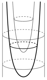
In Figure 1 we study the evolution of a graph over $B_{1}(0)$ (drawn with thick lines), that is asymptotic to the cylinder ${\mathbb{S}}^{n}\times{\mathbb{R}}$ (drawn with grey lines). The thinner lines indicate how the graph looks at some later time. We remark that it continues to be asymptotic to the evolving cylinder, which collapses in finite time. As we prove in Theorem 8.2, the evolving graph does not become singular and it has to disappear to infinity at or before the time the cylinder collapses. Theorem 9.1 implies that the evolving graph and the evolving cylinder disappear at the same time. Notice that near the singular time, the lowest point moves arbitrarily large distances in arbitrarily small time intervals.

Figure 2. Graph over a set that develops a “neck-pinch”

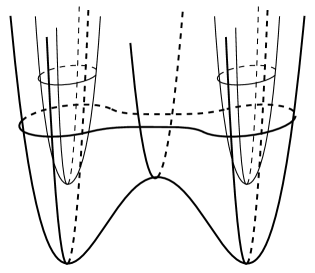
Figure 2 illustrates a graph over a set that develops a “neck-pinch” at $t=T$. This is projected to lower dimensions. For $t\nearrow T$, the graph splits above the “neck-pinch” into two disconnected components without becoming singular. The thinner lines illustrate the graph for $t>T$. The rest of the evolution is similar to the situation above.

Figure 3. Graph defined initially over an annulus

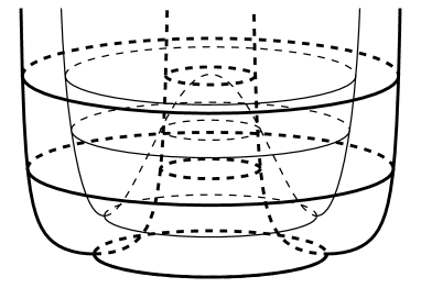
Next, we consider a rotationally symmetric graph over an annulus, centered at the origin, see Figure 3. The inner boundary of the annulus converges to a point as $t\nearrow T$. At $t=T$ a “cap at infinity” is being added to the evolving graph. This cap moves down very quickly. By comparison with compact solutions we see that $u(0,t)$ is finite for any $t>T$. This is illustrated with thin lines. Finally, once again the evolution becomes similar to the evolution in Figure 1.

Figure 4. Domain with nontrivial topology

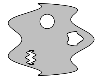
Similarly, when a graph over a domain as in Figure 4 evolves, “caps at infinity” are being added at the times when the small “holes” shrink to points.

Strategy of proof

In order to prove existence of smooth solutions, we start by deriving a priori estimates. The proof of these a priori estimates is based on the observation that powers of the height function can be used to localize derivative estimates in space. Then the result follows by applying these estimates to approximate solutions and employing an Arzelà-Ascoli-type theorem to pass to a limit.

The connection between singularity resolving and weak solutions is obtained as follows: We observe that the cylinder $(\partial\Omega_{t}\times{\mathbb{R}})_{t}$ acts as an outer barrier for $\operatorname{graph}u(\cdot,t)$. Furthermore, since $\operatorname{graph}u(\cdot,t)-R$ converges to the cylinder as $R\to\infty$, we conclude that $\operatorname{graph}u(\cdot,t)$ does not detach from the evolving cylinder near infinity.

Literature

The existence of entire graphs evolving by mean curvature flow was proved by K. Ecker and G. Huisken [11] for Lipschitz continuous initial data and by J. Clutterbuck [6], T. Colding and W. Minicozzi [8] for continuous initial data. K. Ecker, G. Huisken [10] and N. Stavrou [29] have studied convergence to homothetically expanding solutions, J. Clutterbuck, O. Schnürer, F. Schulze [5] and A. Hammerschmidt [20] have investigated stability of entire solutions.

Many authors have worked on weak formulations for mean curvature flow, e. g. K. Brakke [3], K. Ecker [9], L. C. Evans, J. Spruck [12, 13, 14, 15], Y. Chen, Y. Giga, S. Goto [4] and T. Ilmanen [25]. In what follows we will refer as weak flow to level set solutions to mean curvature flow in the sense of Appendix A, see also [4, 12, 21].

Smooth solutions and one additional dimension have been used by S. Altschuler, M. Grayson [1] for curves to extend the evolution past singularities and by T. Ilmanen [24] for the ${\varepsilon}$-regularization of mean curvature flow.

Several people have studied mean curvature flow after the first singularity. We mention a few papers addressing this issue: J. Head [21] and J. Lauer [26] have shown that an appropriate limit of mean curvature flows with surgery (see G. Huisken and C. Sinestrari [22] for the definition of mean curvature flow with surgery) converges to a weak solution. T. Colding and W. Minicozzi [7] consider generic initial data that develop only singularities that look spherical or cylindrical. In the rotationally symmetric case, Y. Giga, Y. Seki and N. Umeda consider mean curvature flow that changes topology at infinity [17, 18].

The height function has been used before in [19] to localize a priori estimates for Monge-Ampère equations.

Organization of the paper

The classical formulation $\dot{X}=-H\nu$ of mean curvature flow does not allow for changes in the topology of the evolving hypersurfaces. Hence in Section 2 we introduce a notion of graphical mean curvature flow that allows for changing domains of definition for the graph function and hence also changes in the topology of the evolving submanifold.

We fix our geometric notation in Section 3 and state evolution equations of geometric quantities in Section 4.

The key ingredients for proving smooth existence are the a priori estimates in Section 5 that use the height function in order to localize the estimates.

In Section 8 we prove existence of smooth solutions. That result follows from combining the Hölder estimates of Section 6 and the compactness result that we prove in Section 7 (a version of the Theorem of Arzelà-Ascoli). In Section 9 we discuss the relationship of our solution and the level set flow solution; we prove Theorem 9.1. Finally, we include an appendix that summarizes some of the results used in Section 9.

Open problems

We wish to mention a few open problems:

1. What is a good description of solutions disappearing at infinity?

2. If the projected solutions or a connected component of the complement become symmetric, e. g. spherical, does the graph pick up that symmetry?

3. What are optimal a priori estimates?

4. Is the solution $(\Omega,u)$ unique?

5. Does the level set solution of $\operatorname{graph}u_{0}$ fatten? Is this fattening related to that of the level set solution of $\partial A$?

Acknowledgment

We want to thank many colleagues for their interest in our work and inspiring discussions: G. Bellettini, K. Ecker, G. Huisken, T. Ilmanen, H. Koch, J. Metzger, F. Schulze, J. Spruck and B. White. Some of these discussions were possible due to invitations to Barcelona, Berlin, Oberwolfach and Potsdam.

2. Definition of a solution

Definition 2.1.

1. Domain of definition: Let $\Omega\subset{\mathbb{R}}^{n+1}\times[0,\infty)$ be a (relatively) open set. Set $\Omega_{t}\mathrel{\mathop{\mathchar 58\relax}}=\pi_{{\mathbb{R}}^{n+1}}\left(\Omega\cap\left({\mathbb{R}}^{n+1}\times\{t\}\right)\right)$, where $\pi_{{\mathbb{R}}^{n+1}}\colon{\mathbb{R}}^{n+2}\to{\mathbb{R}}^{n+1}$ is the projection to the first $n+1$ components. Notice here that the first $n+1$ components of the domain $\Omega$ are spatial, while the last component can be understood as the time component.

   Observe that for each fixed $t$ the section $\Omega_{t}\subset{\mathbb{R}}^{n+1}$ is relatively open.

2. The solution: A function $u\colon\Omega\to{\mathbb{R}}$ is called a classical solution to graphical mean curvature flow in $\Omega$ with continuous initial value $u_{0}\colon\Omega_{0}\to{\mathbb{R}}$, if

   $$u\in C^{2;1}_{\text{loc}}(\Omega\setminus(\Omega_{0}\times\{0\}))\cap C^{0}_{\text{loc}}(\Omega)$$

   where we recall the definition of the spaces below and

   (MCF) $$\begin{cases}\dot{u}=\sqrt{1+|Du|^{2}}\cdot\operatorname{div}\left({\frac{\displaystyle Du}{\displaystyle\sqrt{1+|Du|^{2}}}}\right)&\text{in }\Omega\setminus(\Omega_{0}\times\{0\}),\\ u(\cdot,0)=u_{0}&\text{in }\Omega_{0}.\end{cases}$$

3. Maximality condition: A function $u\colon\Omega\to{\mathbb{R}}$ fulfills the maximality condition if $u\geq-c$ for some $c\in{\mathbb{R}}$ and if $u|_{\Omega\cap\left({\mathbb{R}}^{n+1}\times[0,T]\right)}$ is proper for every $T>0$.

   An initial value $u_{0}\colon\Omega_{0}\to{\mathbb{R}}$, $\Omega_{0}\subset{\mathbb{R}}^{n+1}$, is said to fulfill the maximality condition if $w\colon\Omega_{0}\times[0,\infty)\to{\mathbb{R}}$ defined by $w(x,t)\mathrel{\mathop{\mathchar 58\relax}}=u_{0}(x)$ fulfills the maximality condition.

4. Singularity resolving solution: A function $u\colon\Omega\to{\mathbb{R}}$ is called a singularity resolving solution to mean curvature flow in dimension $n$ with initial value $u_{0}\colon\Omega_{0}\to{\mathbb{R}}$ if

   1. $\Omega$ and $\Omega_{0}$ are as in (i),

   2. $u$ is a classical solution to graphical mean curvature flow with initial value $u_{0}$ as in (ii) and

   3. $u$ fulfills the maximality condition.

5. We do not only call $u$ a singularity resolving solution but also the pair $(\Omega,u)$ and the family $(M_{t})_{t\geq 0}$ with $M_{t}=\operatorname{graph}u(\cdot,t)\subset{\mathbb{R}}^{n+2}$.

Remark 2.2.

1. Note that the domain of definition will depend on the solution.

   The dimensions seem to be artificially increased by one. This is due to the fact that we wish to study the evolution of $(\partial\Omega_{t})_{t\geq 0}$, which in the smooth case, see Remark 9.9 (v), is a family of $n$-dimensional hypersurfaces in ${\mathbb{R}}^{n+1}$ solving mean curvature flow.

2. If $\Omega={\mathbb{R}}^{n+1}$ then condition (ii) in Definition 2.1 coincides with the definition in [11].

   We avoid writing a solution as a family of embeddings $X\colon M\to{\mathbb{R}}^{n+2}$ as in general, the topology of $M$ is not fixed when $\Omega_{t}$ becomes singular.

   We expect similar results for other normal velocities, for example, if $u$ is a singularity resolving solution for the normal velocity $S_{k}$ in dimension $n$ then

   $$\dot{u}=\sqrt{1+|Du|^{2}}\cdot S_{k}[u]\quad\text{in }\Omega\setminus(\Omega_{0}\times\{0\}),$$

   where $S_{k}[u]$ denotes the $k$-th elementary symmetric function of the $n+1$ principal curvatures of graph $u(\cdot,t)\subset{\mathbb{R}}^{n+2}$ and $\Omega$ is as in Definition 2.1 (i).

3. 1. The maximality condition implies that $u$ tends to infinity if we approach a point in the relative boundary $\partial\Omega$. It also ensures that $u(x,t)$ tends to infinity as $|x|$ tends to infinity.

      Hence the maximality allows us to use the height function $u$ for localizing our a priori estimates.

   2. Our maximality condition implies that each graph

      $$M_{t}=\operatorname{graph}u(\cdot,t)\subset{\mathbb{R}}^{n+2}$$

      is a complete submanifold.

   3. If $u$ fulfills the maximality condition then $u_{0}(x)\mathrel{\mathop{\mathchar 58\relax}}=u(x,0)$ also fulfills the maximality condition.

   4. The maximality condition prevents solutions from stopping or starting suddenly. Furthermore, in general restrictions of the domain $\Omega$ of a singularity resolving solution $(\Omega,u)$ do not provide other singularity resolving solutions, i. e. for general open sets $B\subset{\mathbb{R}}^{n+1}\times[0,\infty)$, the pair $(\Omega\cap B,u|_{B})$ does not fulfill the maximality condition.

4. It suffices to study classical solutions to mean curvature flow to obtain singularity resolving solutions. Nevertheless, this allows to obtain weak solutions starting with $\partial\Omega_{0}$ by considering the projections of the evolving graphs.

3. Differential geometry of submanifolds

We use $X=X(x,\,t)=\left(X^{\alpha}\right)_{1\leq\alpha\leq n+2}$ to denote the time-dependent embedding vector of a manifold $M^{n+1}$ into ${\mathbb{R}}^{n+2}$ and ${\frac{d}{dt}}X=\dot{X}$ for its total time derivative. Set $M_{t}\mathrel{\mathop{\mathchar 58\relax}}=X(M,\,t)\subset{\mathbb{R}}^{n+2}$. We will often identify an embedded manifold with its image. We will assume that $X$ is smooth. Assume furthermore that $M^{n+1}$ is smooth, orientable, complete and $\partial M^{n+1}=\emptyset$. We also use that notation if we have that situation only locally, e. g. when the topology changes at spatial infinity.

We choose $\nu=\nu(x)=\left(\nu^{\alpha}\right)_{1\leq\alpha\leq n+2}$ to be the downward pointing unit normal vector to $M_{t}$ at $x$. The embedding $X(\cdot,\,t)$ induces at each point of $M_{t}$ a metric $({g}_{ij})_{1\leq i,\,j\leq n+1}$ and a second fundamental form $(h_{ij})_{1\leq i,\,j\leq n+1}$. Let $\left(g^{ij}\right)$ denote the inverse of $(g_{ij})$. These tensors are symmetric and the principal curvatures $(\lambda_{i})_{1\leq i\leq n+1}$ are the eigenvalues of the second fundamental form with respect to that metric. As usual, eigenvalues are listed according to their multiplicity.

Latin indices range from $1$ to $n+1$ and refer to geometric quantities on the surface, Greek indices range from $1$ to $n+2$ and refer to components in the ambient space ${\mathbb{R}}^{n+2}$. In ${\mathbb{R}}^{n+2}$, we will always choose Euclidean coordinates with fixed $e_{n+2}$-axis. We use the Einstein summation convention for repeated upper and lower indices. Latin indices are raised and lowered with respect to the induced metric or its inverse $\left(g^{ij}\right)$, while for Greek indices we use the flat metric $(\overline{g}_{\alpha\beta})_{1\leq\alpha,\beta\leq n+2}=(\delta_{\alpha\beta})_{1\leq\alpha,\beta\leq n+2}$ of ${\mathbb{R}}^{n+2}$.

Denoting by $\langle\cdot,\,\cdot\rangle$ the Euclidean scalar product in ${\mathbb{R}}^{n+1}$, we have

$$g_{ij}=\left\langle X_{,\,i},\,X_{,\,j}\right\rangle=X^{\alpha}_{,\,i}\delta_{\alpha\beta}X^{\beta}_{,\,j},$$

where we use indices preceded by commas to denote partial derivatives. We write indices preceded by semi-colons, e. g. $h_{ij;\,k}$ or $v_{;k}$, to indicate covariant differentiation with respect to the induced metric. Later, we will also drop the semi-colons and commas, if the meaning is clear from the context. We set $X^{\alpha}_{;i}\equiv X^{\alpha}_{,i}$ and

(3.1) $$X^{\alpha}_{;\,ij}=X^{\alpha}_{,\,ij}-\Gamma^{k}_{ij}X^{\alpha}_{,\,k},$$

where

$$\Gamma^{k}_{ij}=\tfrac{1}{2}g^{kl}(g_{il,\,j}+g_{jl,\,i}-g_{ij,\,l})$$

are the Christoffel symbols of the metric $(g_{ij})$. So $X^{\alpha}_{;ij}$ becomes a tensor.

The Gauß formula relates covariant derivatives of the position vector to the second fundamental form and the normal vector

(3.2) $$X^{\alpha}_{;\,ij}=-h_{ij}\nu^{\alpha}.$$

The Weingarten equation allows to compute derivatives of the normal vector

(3.3) $$\nu^{\alpha}_{;\,i}=h^{k}_{i}X^{\alpha}_{;\,k}.$$

We can use the Gauß formula (3.2) or the Weingarten equation (3.3) to compute the second fundamental form.

Symmetric functions of the principal curvatures are well-defined, we will use the mean curvature $H=\lambda_{1}+\ldots+\lambda_{n+1}$ and the square of the norm of the second fundamental form $|A|^{2}=\lambda_{1}^{2}+\ldots+\lambda_{n+1}^{2}$.

Our sign conventions imply that $H>0$ for the graph of a strictly convex function.

The space $C^{k,\alpha;k/2,\alpha/2}$ denotes the space of functions for which up to $k$-th derivatives are continuous, where time derivatives count twice, these derivatives are Hölder continuous with exponent $\alpha$ in space and $\alpha/2$ in time and the corresponding Hölder norm is finite. The space $C^{k}_{loc}(\Omega)$ consists of the functions $u\colon\Omega\to{\mathbb{R}}$ which are in $C^{k}(K)$ for every $K\Subset\Omega$. We use similar definitions for other (Hölder) spaces.

Finally, we use $c$ to denote universal, estimated constants.

4. Evolution equations for mean curvature flow

Definition 4.1.

If $M$ is given as an embedding and a graph, we use $\eta=(0,\ldots,0,1)$ to denote the vector $e_{n+2}$. The definitions of $\nu$, $H$ and $|A|^{2}$ are as introduced in the previous section. We denote the induced connection by $\nabla$ and the associated Laplace-Beltrami operator by $\Delta$.

We define $v=\left(-\eta_{\alpha}\nu^{\alpha}\right)^{-1}$ and $u=\eta_{\alpha}X^{\alpha}$. The function $u$ can be regarded as a function defined on a subset of ${\mathbb{R}}^{n+1}\times[0,\infty)$ or as a function defined on the evolving manifold $M$. It should be clear from the context which definition of $u$ is being used.

Theorem 4.2.

Let $X$ be a solution to mean curvature flow. Then we have the following evolution equations.

$$\left(\tfrac{d}{dt}-\Delta\right)u= \,0,{}$$

$$\left(\tfrac{d}{dt}-\Delta\right)v= \,-v|A|^{2}-\tfrac{2}{v}|\nabla v|^{2},{}$$

$$\left(\tfrac{d}{dt}-\Delta\right)|A|^{2}= \,-2|\nabla A|^{2}+2|A|^{4},{}$$

$$\left(\tfrac{d}{dt}-\Delta\right)\left|\nabla^{m}A\right|^{2}\leq \,-2\left|\nabla^{m+1}A\right|^{2}$$

$$\,\quad+c(m,n)\cdot\sum\limits_{i+j+k=m}\left|\nabla^{m}A\right|\cdot\left|\nabla^{i}A\right|\cdot\left|\nabla^{j}A\right|\cdot\left|\nabla^{k}A\right|,{}$$

$$\left(\tfrac{d}{dt}-\Delta\right){\mathcal{G}}\leq \,-2k{\mathcal{G}}^{2}-2{\varphi}v^{-3}\langle\nabla v,\nabla{\mathcal{G}}\rangle,$$

where ${\mathcal{G}}={\varphi}|A|^{2}\equiv\frac{v^{2}}{1-kv^{2}}|A|^{2}$ and $k>0$ is chosen so that $kv^{2}\leq\frac{1}{2}$ in the domain considered.

We remark that whenever we use evolution equations from this theorem, we consider $u$ as a function defined on the evolving manifold.

Proof.

See [9, 11]. ∎

5. A priori estimates

The following assumption shall guarantee that we can prove local a priori estimates for the part of $\operatorname{graph}u$ where $u<0$. Notice that, via considering the evolution given by $u-a$ (where $a$ is a constant abbreviating the Spanish word “altura”), this is equivalent to obtain bounds in the set where $u<a$.

In this section we will consider the set $\hat{\Omega}=\{u<0\}$. More precisely, we will work under the following assumption:

Assumption 5.1.

Let $\hat{\Omega}\subset{\mathbb{R}}^{n+1}\times[0,\infty)$ be an open set. Let $u\colon\hat{\Omega}\to{\mathbb{R}}$ be a smooth graphical solution to

$$\dot{u}=\sqrt{1+|Du|^{2}}\cdot\operatorname{div}\left(\frac{Du}{\sqrt{1+|Du|^{2}}}\right)\quad\text{in}\quad\hat{\Omega}\cap\left({\mathbb{R}}^{n+1}\times(0,\infty)\right).$$

Suppose that $u(x,t)\to 0$ as $(x,t)\to(x_{0},t_{0})\in\partial\hat{\Omega}$. Assume that all derivatives of $u$ are uniformly bounded and can be extended continuously across the boundary for all domains $\hat{\Omega}\cap\left({\mathbb{R}}^{n+1}\times[0,T]\right)$ and that these sets are bounded for any $T>0$.

Remark 5.2.

1. Assumption 5.1 is fulfilled for smooth entire solutions $u$ to graphical mean curvature flow that fulfill $u\geq L\geq 1$ outside a compact set when we restrict $u$ to $\hat{\Omega}=\left\{(x,t)\in{\mathbb{R}}^{n+1}\times[0,\infty)\colon u(x,t)<0\right\}$.

2. The approximate solutions $u^{L}_{{\varepsilon},R}$ in Lemma 8.1 fulfill Assumption 5.1 for $L>0$.

3. The following a priori estimates extend to the situation when

   $$\hat{\Omega}=\{(x,t)\colon u(x,t)<a\}$$

   for any $a\in{\mathbb{R}}$ instead of $0$. We only have to replace $u$ by $(u-a)$ below, e. g. in Theorem 5.3.

4. The boundedness assumption of the sets follows from the properness of the function $u$.

Theorem 5.3 ($C^{1}$-estimates).

Let $u$ be as in Assumption 5.1. Then

$$vu^{2}\leq\max\limits_{\genfrac{}{}{0.0pt}{}{t=0}{\{u<0\}}}vu^{2}$$

at points where $u<0$.

Here and in what follows, it is often possible to increase the exponent of $u$.

Proof.

According to Theorem 4.2, $w\mathrel{\mathop{\mathchar 58\relax}}=vu^{2}$ fulfills

$$\dot{w}= \,\dot{v}u^{2}+2vu\dot{u},{}$$

$$w_{i}= \,v_{i}u^{2}+2vuu_{i},{}$$

$$w_{ij}= \,v_{ij}u^{2}+2vuu_{ij}+2vu_{i}u_{j}+2u(v_{i}u_{j}+v_{j}u_{i}),{}$$

$$\left(\tfrac{d}{dt}-\Delta\right)w= \,u^{2}\left(\tfrac{d}{dt}-\Delta\right)v-2v|\nabla u|^{2}-4u\langle\nabla v,\nabla u\rangle$$

$$= \,u^{2}\left(-v|A|^{2}-\tfrac{2}{v}|\nabla v|^{2}\right)-2v|\nabla u|^{2}-4\left\langle\tfrac{u}{\sqrt{v}}\nabla v,\sqrt{v}\nabla u\right\rangle{}$$

$$\leq \,-u^{2}v|A|^{2}\leq 0.$$

The estimate follows from the maximum principle applied to $w$ in the domain where $u<0$. ∎

Remark 5.4.

If the reader prefers to consider a positive cut-off function $(-u)$, we recommend to rewrite Theorem 5.3 as an estimate for $v\cdot(-u)^{2}$.

Corollary 5.5.

Let $u$ be as in Assumption 5.1. Then

$$v\leq\max\limits_{\genfrac{}{}{0.0pt}{}{t=0}{\{u<0\}}}vu^{2}$$

at points where $u\leq-1$.

Remark 5.6.

Similar corollaries also hold for higher derivatives. We do not write them down explicitly.

Remark 5.7.

For later use, we estimate derivatives of $u$ and $v$,

$$|\nabla u|^{2}= \,\eta_{\alpha}X^{\alpha}_{i}g^{ij}X^{\beta}_{j}\eta_{\beta}=\eta_{\alpha}\left(\delta^{\alpha\beta}-\nu^{\alpha}\nu^{\beta}\right)\eta_{\beta}=1-v^{-2}\leq 1$$

and, according to (3.3),

$$|\nabla v|^{2}= \,\left(\left(-\eta_{\alpha}\nu^{\alpha}\right)^{-1}\right)_{i}g^{ij}\left(\left(-\eta_{\beta}\nu^{\beta}\right)^{-1}\right)_{j}=v^{4}\eta_{\alpha}X^{\alpha}_{k}h^{k}_{i}g^{ij}h^{l}_{j}X^{\beta}_{l}\eta_{\beta}\leq v^{4}|A|^{2}$$

$$\leq \,v^{2}{\varphi}|A|^{2}=v^{2}{\mathcal{G}}.$$

So we get

$$|\langle\nabla u,\nabla v\rangle|\leq \,|\nabla u|\cdot|\nabla v|\leq v^{2}|A|\leq v\sqrt{\mathcal{G}}.$$

Theorem 5.8 ($C^{2}$-estimates).

Let $u$ be as in Assumption 5.1.

1. Then there exist $\lambda>0$, $c>0$ and $k>0$ (the constant in ${\varphi}$ and implicitly in ${\mathcal{G}}$), depending on the $C^{1}$-estimates, such that

   $$tu^{4}{\mathcal{G}}+\lambda u^{2}v^{2}\leq\sup\limits_{\genfrac{}{}{0.0pt}{}{t=0}{\{u<0\}}}\lambda u^{2}v^{2}+ct$$

   at points where $u<0$ and $0<t\leq 1$.

2. Moreover, if $u$ is in $C^{2}$ initially, we get $C^{2}$-estimates up to $t=0$: Then there exists $c>0$, depending only on the $C^{1}$-estimates, such that

   $$u^{4}{\mathcal{G}}\leq\sup\limits_{\genfrac{}{}{0.0pt}{}{t=0}{\{u<0\}}}u^{4}{\mathcal{G}}+ct$$

   at points where $u<0$.

Proof.

In order to prove both parts simultaneously, we underline terms and factors that can be dropped everywhere. We get the first part if we consider the underlined terms and the second part if we drop those and set $\lambda=0$.

We set

$$w\mathrel{\mathop{\mathchar 58\relax}}=\underline{t}u^{4}{\mathcal{G}}+\lambda u^{2}v^{2}$$

and obtain

$$\dot{w}= \,\underline{u^{4}{\mathcal{G}}}+4\underline{t}u^{3}{\mathcal{G}}\dot{u}+\underline{t}u^{4}\dot{\mathcal{G}}+2\lambda v^{2}u\dot{u}+2\lambda u^{2}v\dot{v},{}$$

$$w_{i}= \,4\underline{t}u^{3}{\mathcal{G}}u_{i}+\underline{t}u^{4}{\mathcal{G}}_{i}+2\lambda v^{2}uu_{i}+2\lambda u^{2}vv_{i},{}$$

$$w_{ij}= \,4\underline{t}u^{3}{\mathcal{G}}u_{ij}+\underline{t}u^{4}{\mathcal{G}}_{ij}+2\lambda v^{2}uu_{ij}+2\lambda u^{2}vv_{ij}+12\underline{t}u^{2}{\mathcal{G}}u_{i}u_{j}$$

$$\,+4\underline{t}u^{3}({\mathcal{G}}_{i}u_{j}+{\mathcal{G}}_{j}u_{i})+2\lambda v^{2}u_{i}u_{j}+2\lambda u^{2}v_{i}v_{j}+4\lambda vu(u_{i}v_{j}+u_{j}v_{i}),{}$$

$$\underline{t}u^{3}\nabla{\mathcal{G}}= \,\frac{1}{u}\nabla w-4\underline{t}u^{2}{\mathcal{G}}\nabla u-2\lambda v^{2}\nabla u-2\lambda uv\nabla v,{}$$

$$\left(\tfrac{d}{dt}-\Delta\right)w\leq \,\underline{u^{4}{\mathcal{G}}}+\underline{t}u^{4}\left(-2k{\mathcal{G}}^{2}-2{\varphi}v^{-3}\langle\nabla v,\nabla{\mathcal{G}}\rangle\right)+2\lambda u^{2}v\left(-v|A|^{2}-\tfrac{2}{v}|\nabla v|^{2}\right)$$

$$\,-12\underline{t}u^{2}{\mathcal{G}}|\nabla u|^{2}-8\underline{t}u^{3}\langle\nabla{\mathcal{G}},\nabla u\rangle-2\lambda v^{2}|\nabla u|^{2}-2\lambda u^{2}|\nabla v|^{2}$$

$$\,-8\lambda uv\langle\nabla u,\nabla v\rangle.$$

In the following, we will use the notation $\langle\nabla w,b\rangle$ for generic gradient terms for the test function $w$. The constants $c$ are allowed to depend on $\sup\{|u|\colon u<0\}$ (which does not exceed its initial value) and the $C^{1}$-estimates which are uniform as we may consider $v\cdot(u-1)^{2}$ in Theorem 5.3. In case (i), it may also depend on an upper bound for $t$, but we assume that $0<t\leq 1$. That is, we suppress dependence on already estimated quantities.

We estimate the terms involving $\nabla{\mathcal{G}}$ separately. Let ${\varepsilon}>0$ be a constant. We fix its value blow. Using Remark 5.7 for estimating terms, we get

$$-2{\varphi}\underline{t}u^{4}v^{-3}\langle\nabla v,\nabla{\mathcal{G}}\rangle= \,-2\frac{{\varphi}u}{v^{3}}\left\langle\nabla v,\frac{1}{u}\nabla w-4\underline{t}u^{2}{\mathcal{G}}\nabla u-2\lambda v^{2}\nabla u-2\lambda uv\nabla v\right\rangle{}$$

$$\leq \,\langle\nabla w,b\rangle+8\underline{t}\frac{{\varphi}u^{3}}{v}{\mathcal{G}}|A|+4\lambda{\varphi}|u|v|A|+4\frac{\lambda{\varphi}u^{2}}{v^{2}}|\nabla v|^{2}{}$$

$$\leq \,\langle\nabla w,b\rangle+{\varepsilon}\underline{t}u^{4}{\mathcal{G}}^{2}+{\varepsilon}\lambda u^{2}v^{2}|A|^{2}+\lambda u^{2}|\nabla v|^{2}\cdot 4\frac{{\varphi}}{v^{2}}+c({\varepsilon},\lambda),{}$$

$$-8\underline{t}u^{3}\langle\nabla{\mathcal{G}},\nabla u\rangle= \,-8\left\langle\nabla u,\frac{1}{u}\nabla w-4\underline{t}u^{2}{\mathcal{G}}\nabla u-2\lambda v^{2}\nabla u-2\lambda uv\nabla v\right\rangle{}$$

$$\leq \,\langle\nabla w,b\rangle+32\underline{t}u^{2}{\mathcal{G}}+16\lambda v^{2}+16\lambda|u|v^{3}|A|{}$$

$$\leq \,\langle\nabla w,b\rangle+{\varepsilon}\underline{t}u^{4}{\mathcal{G}}^{2}+{\varepsilon}\lambda u^{2}v^{2}|A|^{2}+c({\varepsilon},\lambda).$$

We obtain

$$\left(\tfrac{d}{dt}-\Delta\right)w\leq \,\underline{u^{4}{\mathcal{G}}}+\underline{t}u^{4}{\mathcal{G}}^{2}(-2k+2{\varepsilon})+\langle\nabla w,b\rangle$$

$$\,+\lambda u^{2}v^{2}|A|^{2}(-2+3{\varepsilon})+\lambda u^{2}|\nabla v|^{2}\left(4\frac{{\varphi}}{v^{2}}-6\right)+c({\varepsilon},\lambda).$$

Let us assume that $k>0$ is chosen so small that $kv^{2}\leq\frac{1}{3}$ in $\{u<0\}$. This implies ${\varphi}\leq 2v^{2}$. We may assume that $\lambda\geq 2u^{2}$ in $\{u<0\}$ and get $u^{4}{\mathcal{G}}\leq\frac{1}{2}\lambda u^{2}{\varphi}|A|^{2}\leq\lambda u^{2}v^{2}|A|^{2}$. We get

$$4\frac{{\varphi}}{v^{2}}-6=\frac{4}{1-kv^{2}}-6\leq 0.$$

Finally, fixing ${\varepsilon}>0$ sufficiently small, we obtain

$$\left(\tfrac{d}{dt}-\Delta\right)w\leq\langle\nabla w,b\rangle+c.$$

Now, both claims follow from the maximum principle. ∎

Theorem 5.9 ($C^{m+2}$-estimates).

Let $u$ be as in Assumption 5.1.

1. There exists $\lambda>0$, depending on the $C^{m+1}$-estimates, such that

   $$tu^{2}\left|\nabla^{m}A\right|^{2}+\lambda\left|\nabla^{m-1}A\right|^{2}\leq c\cdot\lambda\cdot t+\sup\limits_{\genfrac{}{}{0.0pt}{}{t=0}{\{u<0\}}}\lambda\left|\nabla^{m-1}A\right|^{2}$$

   at points where $u<0$ and $0<t\leq 1$.

2. As in Theorem 5.8, initial smoothness is preserved.

Remark 5.10.

1. This implies a priori estimates for arbitrary derivatives and any $t>0$: It is known that estimates for $u$, $v$, $|A|$ and $\left|\nabla^{m}A\right|$, $1\leq m\leq M$, imply (spatial) $C^{M+2}$-estimates for the function that represents the evolving hypersurface as a graph. Using the equation, we can bound time derivatives.

2. For estimates at time $t_{0}>1$, we can use the previous theorems with $t=0$ replaced by $t=t_{0}-1/2$.

3. To control the $m$-th (spatial) derivative at time $t_{0}>0$, we can apply the result iteratively and control the $k$-th derivatives, $1\leq k\leq m$, at time $\frac{kt_{0}}{m}$.

4. Theorem 5.9 implies smoothness for $t>0$. We do not expect, however, that the decay rates obtained for $\left|\nabla^{m}A\right|^{2}$ are optimal near $t=0$.

Proof of Theorem 5.9.

Once again, we underline terms and factors that can be dropped to obtain uniform estimates up to $t=0$. We define

$$w\mathrel{\mathop{\mathchar 58\relax}}=\underline{t}u^{2}\left|\nabla^{m}A\right|^{2}+\lambda\left|\nabla^{m-1}A\right|^{2}$$

for a constant $\lambda>0$ to be fixed. We will assume that $\left|\nabla^{k}A\right|^{2}$ is already controlled for any $0\leq k\leq m-1$. Suppose that $0\leq t\leq 1$. The constant $c$ is allowed to depend on quantities that we have already controlled. Thus the evolution equation for $\left|\nabla^{m}A\right|^{2}$ in Theorem 4.2 becomes for $m\geq 1$

$$\left(\tfrac{d}{dt}-\Delta\right)\left|\nabla^{m}A\right|^{2}\leq \,-2\left|\nabla^{m+1}A\right|^{2}+c\left|\nabla^{m}A\right|^{2}+c,{}$$

$$\left(\tfrac{d}{dt}-\Delta\right)\left|\nabla^{m-1}A\right|^{2}\leq \,-2\left|\nabla^{m}A\right|^{2}+c.$$

We get

$$\dot{w}= \,\underline{u^{2}\left|\nabla^{m}A\right|^{2}}+2\underline{t}u\dot{u}\left|\nabla^{m}A\right|^{2}+\underline{t}u^{2}{\frac{d}{dt}}\left|\nabla^{m}A\right|^{2}+\lambda{\frac{d}{dt}}\left|\nabla^{m-1}A\right|^{2},{}$$

$$w_{i}= \,2\underline{t}uu_{i}\left|\nabla^{m}A\right|^{2}+\underline{t}u^{2}\left(\left|\nabla^{m}A\right|^{2}\right)_{i}+\lambda\left(\left|\nabla^{m-1}A\right|^{2}\right)_{i},{}$$

$$w_{ij}= \,2\underline{t}uu_{ij}\left|\nabla^{m}A\right|^{2}+\underline{t}u^{2}\left(\left|\nabla^{m}A\right|^{2}\right)_{ij}+\lambda\left(\left|\nabla^{m-1}A\right|^{2}\right)_{ij}$$

$$\,+2\underline{t}u_{i}u_{j}\left|\nabla^{m}A\right|^{2}+2\underline{t}u\left(u_{i}\left(\left|\nabla^{m}A\right|^{2}\right)_{j}+u_{j}\left(\left|\nabla^{m}A\right|^{2}\right)_{i}\right),{}$$

$$\left(\tfrac{d}{dt}-\Delta\right)w\leq \,\underline{u^{2}\left|\nabla^{m}A\right|^{2}}+\underline{t}u^{2}\left(-2\left|\nabla^{m+1}A\right|^{2}+c\left|\nabla^{m}A\right|^{2}+c\right)$$

$$\,+\lambda\left(-2\left|\nabla^{m}A\right|^{2}+c\right)-2\underline{t}|\nabla u|^{2}\left|\nabla^{m}A\right|^{2}-4\underline{t}u\left\langle\nabla u,\nabla\left|\nabla^{m}A\right|^{2}\right\rangle.$$

We observe that

$$-4\underline{t}u\left\langle\nabla u,\nabla\left|\nabla^{m}A\right|^{2}\right\rangle\leq\underline{t}\cdot|u|\cdot c\cdot\left|\nabla^{m+1}A\right|\cdot\left|\nabla^{m}A\right|\leq\underline{t}u^{2}\left|\nabla^{m+1}A\right|^{2}+c\left|\nabla^{m}A\right|^{2}.$$

Therefore we get

$$\left(\tfrac{d}{dt}-\Delta\right)w\leq\left(c-2\lambda\right)\left|\nabla^{m}A\right|^{2}+c(\lambda)$$

and the result follows from the maximum principle. ∎

6. Hölder estimates in time

We will use the following Hölder estimates to prove maximality of a limit of solutions.

Lemma 6.1.

Let $u\colon{\mathbb{R}}^{n+1}\times[0,\infty)\to{\mathbb{R}}$ be a graphical solution to mean curvature flow and $M\geq 1$ such that

$$|Du(x,t)|\leq M\quad\text{for all $(x,t)$ where }\quad u(x,t)\leq 0.$$

Fix any $x_{0}\in{\mathbb{R}}^{n+1}$ and $t_{1},t_{2}\geq 0$. If $u(x_{0},t_{1})\leq-1$ or $u(x_{0},t_{2})\leq-1$, then $|t_{1}-t_{2}|\geq\frac{1}{8(n+1)M^{2}}$ or

$$\frac{|u(x_{0},t_{1})-u(x_{0},t_{2})|}{\sqrt{|t_{1}-t_{2}|}}\leq\sqrt{2(n+1)}(M+1).$$

The previous lemma implies that $u$ is locally uniformly Hölder continuous in time. Although Lemma 6 follows from the bounds for $H$ provided by [11, Theorem 3.1], we include below an independent and more elementary proof which employs spheres as barriers.

Proof.

We may assume that $t_{1}\leq t_{2}$.

1. Assume first that $u(x_{0},t_{1})\leq-1$. As $|Du(x,t)|\leq M$ for $u(x,t)\leq 0$, we deduce for any $0<r\leq\frac{1}{M}$

   $$u(x_{0},t_{1})-Mr\leq u(y,t_{1})\leq u(x_{0},t_{1})+Mr\quad\text{for all }y\in B^{n+1}_{r}(x_{0}).$$

   Hence the sphere $\partial B_{r}^{n+2}(x_{0},u(x_{0},t_{1})+(M+1)r)$ lies above $\operatorname{graph}u(\cdot,t_{1})$ and $\partial B_{r}^{n+2}(x_{0},u(x_{0},t_{1})-(M+1)r)$ lies below $\operatorname{graph}u(\cdot,t_{1})$. When the spheres evolve by mean curvature flow, their radii are given by

   $$r(t)=\sqrt{r^{2}-2(n+1)(t-t_{1})}$$

   for $t_{1}\leq t<t_{1}+\frac{r^{2}}{2(n+1)}$. Both spheres are compact solutions to mean curvature flow. Hence they are barriers for $\operatorname{graph}u(\cdot,t)$. In particular, we get

   $$u(x_{0},t_{1})-(M+1)r\leq u\left(x_{0},t_{1}+\frac{r^{2}}{2(n+1)}\right)\leq u(x_{0},t_{1})+(M+1)r.$$

   Set $r\mathrel{\mathop{\mathchar 58\relax}}=\sqrt{2(n+1)(t_{2}-t_{1})}$. We may assume $|t_{1}-t_{2}|\leq\frac{1}{2(n+1)M^{2}}$. Hence $r\leq\frac{1}{M}$ and the considerations above apply. We obtain

   $$u(x_{0},t_{1})-(M+1)\sqrt{2(n+1)(t_{2}-t_{1})}\leq \,u(x_{0},t_{2})$$

   $$\leq \,u(x_{0},t_{1})+(M+1)\sqrt{2(n+1)(t_{2}-t_{1})}.$$

   Rearranging implies the Hölder continuity claimed above.

2. Assume now that $u(x_{0},t_{2})\leq-1$ and $u(x_{0},t_{1})>-1$. We argue by contradiction: Suppose that $t_{2}\geq t_{1}\geq t_{2}-\frac{1}{8(n+1)M^{2}}$ and

   (6.1) $$\frac{u(x_{0},t_{1})-u(x_{0},t_{2})}{\sqrt{t_{2}-t_{1}}}\geq\sqrt{2(n+1)}(M+1).$$

   Set $r\mathrel{\mathop{\mathchar 58\relax}}=\sqrt{2(n+1)(t_{2}-t_{1})}$. We claim that

   (6.2) $$\min\{u(x_{0},t_{1}),0\}-Mr\geq u(x_{0},t_{2})+r.$$

   If $u(x_{0},t_{1})<0$, (6.2) follows by rearranging (6.1). Otherwise, we have that

   $$u(x_{0},t_{2})+(M+1)r\leq \,-1+(M+1)\sqrt{2(n+1)(t_{2}-t_{1})}$$

   $$\leq \,-1+(M+1)\sqrt{\frac{2(n+1)}{8(n+1)M^{2}}}\leq-1+\frac{M+1}{2M}\leq 0$$

   as $M\geq 1$. This proves claim (6.2).

   Now, using (6.2), we can proceed similarly as in (i): For some small ${\varepsilon}>0$, the sphere $\partial B^{n+2}_{r}(x_{0},u(x_{0},t_{2})+{\varepsilon})$ lies below $\operatorname{graph}u(\cdot,t_{1})$ (for the positivity of ${\varepsilon}$ consider in (6.2) the terms $-Mr$ near the center and $+r$ near the boundary). Under mean curvature flow, the sphere shrinks to a point as $t\nearrow t_{2}$ and stays below $\operatorname{graph}u(\cdot,t)$. We obtain $u(x_{0},t_{2})+{\varepsilon}\leq u(x_{0},t_{2})$, which is a contradiction. ∎

7. Compactness results

Lemma 7.1.

Let $\Omega\subset B\subset{\mathbb{R}}^{n+2}$ and consider a function $u\colon\Omega\to{\mathbb{R}}$. Assume that for each $a\in{\mathbb{R}}$ there exists $r(a)>0$ such that for each $x\in\Omega$ with $u(x)\leq a$ we have $B_{r(a)}(x)\cap B\subset\Omega$. Then $\Omega$ is relatively open in $B$ and $u(x_{k})\to\infty$ if $x_{k}\to x\in\partial\Omega$, where $\partial\Omega$ is the relative boundary of $\Omega$ in $B$.

Proof.

It is clear that $\Omega\subset B$ is relatively open. If $u$ were not tending to infinity near the boundary, we find $x_{n}\in\Omega$ such that $x_{n}\to x\in\partial\Omega$ as $n\to\infty$ and $u(x_{n})\leq a$ for some $a\in{\mathbb{R}}$. Since $B_{r(a)}(x_{n})\cap B\subset\Omega$, the triangle inequality implies $x\in B_{r(a)}(x_{n})$ for $n$ sufficiently large. This contradicts $x\in\partial\Omega$. ∎

Remark 7.2.

A continuous maximal graph is a closed set and – if sufficiently smooth – a complete manifold.

Lemma 7.3 (Variation on the Theorem of Arzelà-Ascoli).

Let $B\subset{\mathbb{R}}^{n+2}$ and $0<\alpha\leq 1$. Let $u_{i}\colon B\to{\mathbb{R}}\cup\{\infty\}$ for $i\in{\mathbb{N}}$. Suppose that there exist strictly decreasing functions $r,\,-c\colon{\mathbb{R}}\to{\mathbb{R}}_{+}$ such that for each $x\in B$ and $i\geq i_{0}(a)$ with $u_{i}(x)\leq a<\infty$ we have

$$\frac{|u_{i}(x)-u_{i}(y)|}{|x-y|^{\alpha}}\leq c(a)\quad\text{for all}\quad y\in\overline{B_{r(a)}(x)}\cap B.$$

Then there exists a function $u\colon B\to{\mathbb{R}}\cup\{\infty\}$ such that a subsequence $(u_{i_{k}})_{k\in{\mathbb{N}}}$ converges to $u$ locally uniformly in $\Omega\mathrel{\mathop{\mathchar 58\relax}}=\{x\in B\colon u(x)<\infty\}$ and $u_{i_{k}}(x)\to\infty$ for $x\in B\setminus\Omega$. Moreover, for each $x\in\Omega$ with $u(x)\leq a$ we have $B_{r(a+1)}(x)\cap B\subset\Omega$ and

$$\frac{|u(x)-u(y)|}{|x-y|^{\alpha}}\leq c(a+1)\quad\text{for all}\quad y\in\overline{B_{r(a+1)}(x)}\cap B.$$

Proof.

We adapt the proof of the Theorem of Arzelà-Ascoli to our situation. Let $D\mathrel{\mathop{\mathchar 58\relax}}=\{x_{l}\colon l\in{\mathbb{N}}\}$ be dense in $B$.

If $\liminf\limits_{i\to\infty}u_{i}(x_{0})<\infty$, we choose a subsequence $(u_{i_{k}})_{k\in{\mathbb{N}}}$, such that $\lim\limits_{k\to\infty}u_{i_{k}}(x_{0})=\liminf\limits_{i\to\infty}u_{i}(x_{0})$. If $\liminf\limits_{i\to\infty}u_{i}(x_{0})=\infty$, we do not need to pass to a subsequence.

Proceed similarly with $x_{1},x_{2},\ldots$ instead of $x_{0}$. We denote the diagonal sequence of this sequence of subsequences by $(\tilde{u}_{i})_{i\in{\mathbb{N}}}$. Define $u(x_{k})\mathrel{\mathop{\mathchar 58\relax}}=\lim\limits_{i\to\infty}\tilde{u}_{i}(x_{k})\in{\mathbb{R}}\cup\{\infty\}$ for $k\in{\mathbb{N}}$. This limit exists by the construction of the subsequence $(\tilde{u}_{i})_{i\in{\mathbb{N}}}$. By passing to the limit in the Hölder estimate for $\tilde{u}_{i}$, we obtain the claimed Hölder estimate with $a+\frac{1}{2}$ for $u$ and $x=x_{k},y=x_{l}$, $k,l\in{\mathbb{N}}$. Set $u(x)\mathrel{\mathop{\mathchar 58\relax}}=\lim\limits_{k\to\infty}u(x_{k})$ for $x\in B$, $x_{k}\in D$ and $x_{k}\to x$ as $k\to\infty$. The Hölder estimate ensures that $u$ is well-defined and fulfills the claimed Hölder estimate with $a+1$. Set $\Omega\mathrel{\mathop{\mathchar 58\relax}}=\{x\in B\colon u(x)<\infty\}$. There, pointwise convergence and local Hölder estimates imply locally uniform convergence in $\Omega$. ∎

Remark 7.4.

1. This result extends to families of locally equicontinuous functions.

2. Notice that the functions $u_{i}$ in the previous lemma are not necessarily finite on all of $B$. Hence the lemma can also be applied to functions $u_{i}$ which are not defined in all of $B$: It suffices to set $u_{i}\mathrel{\mathop{\mathchar 58\relax}}=+\infty$ outside its original domain of definition.

3. Observe that the domain $\Omega$ obtained in Lemma 7.3 may be empty. However, for the existence result (Theorem 8.2), the fact that $\Omega\neq\emptyset$ is ensured by the choice of initial condition for the approximating solutions and Lemma 6.1.

8. Existence

In this section we will use approximate solutions to prove existence of a singularity resolving solution to mean curvature flow.

We start by constructing a nice mollification of $\min\{\cdot,\cdot\}$. Choose a smooth monotone approximation $f$ of $\min\{\cdot,0\}$ such that $f(x)=\min\{x,0\}$ for $|x|>1$ and set $\min_{\varepsilon}\{a,b\}\mathrel{\mathop{\mathchar 58\relax}}={\varepsilon}f\left(\frac{1}{{\varepsilon}}(a-b)\right)+b$.

We will set $\min_{\varepsilon}\{u(x),L\}\mathrel{\mathop{\mathchar 58\relax}}=L$ at $x$ if $u$ is not defined at $x$.

Lemma 8.1 (Existence of approximating solutions).

Let $A\subset{\mathbb{R}}^{n+1}$ be an open set. Assume that $u_{0}\colon A\to{\mathbb{R}}$ is locally Lipschitz continuous and maximal.

Let $L>0$, $R>0$ and $1\geq{\varepsilon}>0$. Then there exists a smooth solution $u_{{\varepsilon},R}^{L}$ to

$$\begin{cases}\dot{u}=\sqrt{1+|Du|^{2}}\cdot\operatorname{div}\left(\dfrac{Du}{\sqrt{1+|Du|^{2}}}\right)&\text{in }B_{R}(0)\times[0,\infty),\\ u=L&\text{on }\partial B_{R}(0)\times[0,\infty),\\ u(\cdot,0)=\min_{\varepsilon}\big{\{}u_{0,{\varepsilon}},L\big{\}}&\text{in }B_{R}(0),\end{cases}$$

where $u_{0,{\varepsilon}}$ is a standard mollification of $u_{0}$. We always assume that $R\geq R_{0}(L,{\varepsilon})$ is so large that $L+1\leq u_{0,{\varepsilon}}$ on $\partial B_{R}(0)$.

Proof.

The initial value problem for $u^{L}_{{\varepsilon},R}$ involves smooth data which fulfill the compatibility conditions of any order for this parabolic problem. Hence we obtain a smooth solution $u^{L}_{{\varepsilon},R}$ for some positive time interval. According to [23], this solution exists for all positive times. ∎

Observe that the approximate solutions of Lemma 8.1 fulfill Assumption 5.1 with

$$\hat{\Omega}=\left\{(x,t)\colon u_{{\varepsilon},R}^{L}<a\right\}$$

and $0$ there replaced by $a$ for any $a<L$.

Theorem 8.2 (Existence).

Let $A\subset{\mathbb{R}}^{n+1}$ be an open set. Assume that $u_{0}\colon A\to{\mathbb{R}}$ is maximal and locally Lipschitz continuous.

Then there exists $\Omega\subset{\mathbb{R}}^{n+1}\times[0,\infty)$ such that $\Omega\cap\left({\mathbb{R}}^{n+1}\times\{0\}\right)=A\times\{0\}$ and a (classical) singularity resolving solution $u\colon\Omega\to{\mathbb{R}}$ with initial value $u_{0}$.

Proof.

Consider the approximate solutions $u^{L}_{{\varepsilon},R}$ given by Lemma 8.1. The a priori estimates of Theorem 5.3 and Lemma 6.1 apply to this situation in $\big{\{}(x,t)\in B_{R}(0)\times[0,\infty)\colon u^{L}_{{\varepsilon},R}(x,t)\leq L-1\big{\}}$. According to [11], we get $u^{L}_{1/i,i}\to u^{L}$ as $i\to\infty$ and $u^{L}$ is a solution to mean curvature flow with initial condition $\min\{u,L\}$.

Let us derive lower bounds for $u^{L}$ that will ensure maximality of the limit when $L\to\infty$. As the initial value $u_{0}$ fulfills the maximality condition for every $r>0$ we can find $d=d(r)$ such that $B_{r}((x,L-r-1))$ lies below $\operatorname{graph}\min\{u,L\}$ if $|x|\geq d$. Hence $u^{L}(x,t)\geq L-2$ for $0\leq t\leq\frac{1}{n+1}r-\frac{1}{2(n+1)}$ if $|x|\geq d$. Therefore for any $T>0$ there exists $d\geq 0$ such that $u^{L}(x,t)\geq L-2$ for $|x|\geq d$ and $0\leq t\leq T$.

The estimates of Theorem 5.3, Theorem 5.8 and Theorem 5.9 survive the limiting process and continue to hold for $u^{L}$: We get locally uniform estimates on arbitrary derivatives of $u^{L}$ in compact subsets of $\Omega\cap\left({\mathbb{R}}^{n+1}\times(0,\infty)\right)$. The estimate of Lemma 6.1 also survives the limiting process and we get uniform bounds for $\left\|u^{L}\right\|_{C^{0,1;0,1/2}}$ in compact subsets of $\Omega$.

Now we apply Lemma 7.3 to $u^{L}$, $L\in{\mathbb{N}}$, and get a solution $(\Omega,u)$ and a subsequence of $u^{L}$, which we assume to be $u^{L}$ itself, such that $u^{L}\to u$ locally uniformly in $\Omega$.

According to Lemma 7.1, $\Omega$ is open in ${\mathbb{R}}^{n+1}\times[0,\infty)$. The $C^{0,1;0,1/2}$-estimates imply that the domains of definition of $u_{0}$ and $u|_{t=0}$ coincide. In particular in Definition 2.1 we get $A=\Omega_{0}(\Omega)$ and $u(\cdot,0)=u_{0}$.

The derivative estimates and local interpolation inequalities of the form

$$\|Dw\|^{2}_{C^{0}(B)}\leq c(n,B)\cdot\|w\|_{C^{0}(B)}\cdot\|w\|_{C^{2}(B)}$$

for any $w\in C^{2}$ and any ball $B$ (see e. g. [27, Lemma A.5]) imply that $u^{L}\to u$ smoothly in $\Omega\cap\left({\mathbb{R}}^{n+1}\times(0,\infty)\right)$. Hence $u$ fulfills the differential equation for graphical mean curvature flow.

The lower bound $u^{L}(x,t)\geq L-2$ above for $|x|\geq d$ and Lemma 7.1 imply maximality.

Hence, we obtain the existence of a singularity resolving solution $(\Omega,u)$ for each maximal Lipschitz continuous function $u_{0}\colon A\to{\mathbb{R}}$. ∎

Remark 8.3.

Notice that in the proof of Theorem 8.2 we started with the approximate solutions of Lemma 8.1 instead of $u^{L}$ in the proof of Theorem 8.2 as the former are smooth up to $t=0$ and allow to apply our a priori estimates.

9. The level set flow and singularity resolving solutions

In this section we explore the relation between level set solutions as defined at the beginning of Appendix A and singularity resolving solutions given by Theorem 8.2. More precisely, we prove the following result

Theorem 9.1.

Let $(\Omega,u)$ be a solution to mean curvature flow as in Theorem 8.2. Let $\partial{\mathcal{D}}_{t}$ be the level set evolution of $\partial\Omega_{0}$ as defined below. If $\partial{\mathcal{D}}_{t}$ does not fatten, the measure theoretic boundaries of $\Omega_{t}$ and ${\mathcal{D}}_{t}$ coincide for every $t\geq 0$: $\partial^{\mu}\Omega_{t}=\partial^{\mu}{\mathcal{D}}_{t}$.

For the definition of a level set solution and fattening, we refer to Appendix A.

In order to prove Theorem 9.1 we need a few definitions which we summarize in Table 1. Unless stated otherwise, we will always assume that we consider signed distance functions which are truncated between $-1$ and $1$, i. e. we consider $\max\{-1,\min\{d,1\}\}$, and negative inside the set or above the graph considered.

1. Let $\tilde{v}\colon{\mathbb{R}}^{n+1}\times[0,\infty)\to{\mathbb{R}}$ be the solution to (A.1) such that $\tilde{v}(\cdot,0)$ is the distance function to $\partial\Omega_{0}$. Set ${\mathcal{D}}_{t}\mathrel{\mathop{\mathchar 58\relax}}=\left\{x\in{\mathbb{R}}^{n+1}\colon\tilde{v}(x,t)<0\right\}$.

2. Let $v\colon{\mathbb{R}}^{n+2}\times[0,\infty)\to{\mathbb{R}}$ be the solution to (A.1) such that $v(\cdot,0)$ is the distance function to $\partial\Omega_{0}\times{\mathbb{R}}$. Set $C_{t}\mathrel{\mathop{\mathchar 58\relax}}=\left\{\left(x,x^{n+2}\right)\in{\mathbb{R}}^{n+2}\colon v\left(x,x^{n+2},t\right)<0\right\}$.

3. Let $w\colon{\mathbb{R}}^{n+2}\times[0,\infty)\to{\mathbb{R}}$ be the solution to (A.1) such that $w(\cdot,0)$ is the distance function to $\operatorname{graph}u(\cdot,0)|_{\Omega_{0}}$. Set $E_{t}\mathrel{\mathop{\mathchar 58\relax}}=\left\{\left(x,x^{n+2}\right)\colon w\left(x,x^{n+2},t\right)<0\right\}$.

solution to (A.1)	initial set	set
$w$	$\operatorname{graph}u_{0}$	$E_{t}$
$\tilde{v}$	$\partial\Omega_{0}$	${\mathcal{D}}_{t}$
$v$	$\partial\Omega_{0}\times{\mathbb{R}}$	$C_{t}$

Table 1. Notation for weak solutions

Theorem 9.1 will follow from

Proposition 9.2.

Let $(\Omega,u)$ be a solution to mean curvature flow as in Theorem 8.2. If the level set evolution of $\partial\Omega_{0}$ does not fatten, we obtain $\mathcal{H}^{n+1}$-almost everywhere that $\Omega_{t}={\mathcal{D}}_{t}$ for all $t\geq 0$, i. e. $\mathcal{H}^{n+1}(\Omega_{t}\triangle{\mathcal{D}}_{t})=0$ for every $t\geq 0$.

We start by showing that $v$ and $\tilde{v}$ are closely related.

Lemma 9.3.

For $v$ and $\tilde{v}$ as above, we have $v\left(x,x^{n+2},t\right)=\tilde{v}(x,t)$ for all points $\left(x,x^{n+2},t\right)\in{\mathbb{R}}^{n+1}\times{\mathbb{R}}\times[0,\infty)$. This implies ${\mathcal{D}}_{t}\times{\mathbb{R}}=C_{t}$ and ${\mathcal{D}}_{t}^{+}\times{\mathbb{R}}=C^{+}_{t}$.

Proof.

This follows directly from uniqueness of solutions to (A.1) as $v\left(x,x^{n+2},0\right)=\tilde{v}(x,0)$. See Theorem A.1. ∎

Lemma 9.4.

We have $w\geq v$. In particular, $E_{t}^{+}\subset C^{+}_{t}$.

Proof.

This follows from $w(\cdot,0)\geq v(\cdot,0)$ and Theorem A.3. ∎

Lemma 9.5.

We have $\operatorname{graph}u(\cdot,t)\subset\partial E^{+}_{t}$.

Proof.

Let $w^{L}\colon{\mathbb{R}}^{n+2}\times[0,\infty)\to{\mathbb{R}}$ be the solution to (A.1) with $w^{L}(\cdot,0)$ equal to the distance function to $\operatorname{graph}u^{L}$, where $u^{L}$ is as in Theorem 8.2. According to [2] the solution $w^{L}$ does not fatten: For each ${\varepsilon}>0$ there is a $\delta>0$ such that the inequality $w^{L}(x,0)\geq w^{L}\left(x+{\varepsilon}e^{n+2},0\right)+\delta$ holds if we truncate at appropriate heights. By Theorem A.2 and Theorem A.3 we have that $w^{L}(x,t)\geq w^{L}\left(x+{\varepsilon}e^{n+2},t\right)+\delta$ near the zero level set. Hence $\left\{\left(x,x^{n+2}\right)\in{\mathbb{R}}^{n+1}\times{\mathbb{R}}\colon w^{L}\left(x,x^{n+2},t\right)=0\right\}=\operatorname{graph}u^{L}(\cdot,t)$.

Observe that $w^{L}(\cdot,0)\nearrow w(\cdot,0)$. Hence Theorem A.4 implies that $w^{L}(\cdot,t)\nearrow w(\cdot,t)$ for all $t\geq 0$.

Let $x^{n+2}<u(x,t)$. Then $x^{n+2}<u^{L}(x,t)$ for some $L$ and hence $w^{L}\left(x,x^{n+2},t\right)>0$. Since $w\left(x,x^{n+2},t\right)\geq w^{L}\left(x,x^{n+2},t\right)>0$ we have that

(9.1) $$\left\{\left(x,x^{n+2}\right)\colon x^{n+2}<u(x,t)\right\}\subset\left\{\left(x,x^{n+2}\right)\colon 0<w\left(x,x^{n+2},t\right)\right\}.$$

On the other hand, for every $\left(x,x^{n+2},t\right)$ such that $x^{n+2}=u(x,t)$ there is a sequence $\left(x,u^{L}(x,t)\right)_{L}$ such that $\left(x,u^{L}(x,t)\right)\to\left(x,u(x,t)\right)$ as $L\to\infty$. Moreover, since the $w^{L}$ converge monotonically, the convergence is locally uniform. We conclude that

$$0=\lim\limits_{L\to\infty}w^{L}\left(x,u^{L}(x,t),t\right)=w\left(x,u(x,t),t\right).$$

This concludes the proof of $\operatorname{graph}u(\cdot,t)\subset\partial E^{+}_{t}$.

By arguments similar to those used for proving (9.1), we can show that

$$\left\{\left(x,x^{n+2}\right)\colon x^{n+2}>u(x,t)\right\}\subset\left\{\left(x,x^{n+2}\right)\colon w\left(x,x^{n+2},t\right)\leq 0\right\}.\qed$$

Corollary 9.6.

Let $x\not\in\Omega_{t}$ then $w\left(x,x^{n+2},t\right)>0$ for any $x^{n+2}$.

Proof.

The above argument in the case $x^{n+2}<u(x,t)$ also extends to the case $u(x,t)=+\infty$. ∎

Corollary 9.7.

If $C_{t}$ or, equivalently, ${\mathcal{D}}_{t}$ does not fatten, then $\Omega_{t}\subset{\mathcal{D}}^{\mu}_{t}$.

Proof.

Combining Lemmata 9.3, 9.4 and 9.5 we get $\operatorname{graph}u(\cdot,t)\subset{\mathcal{D}}_{t}^{+}\times{\mathbb{R}}$. This implies $\Omega_{t}\subset{\mathcal{D}}_{t}^{+}$. As ${\mathcal{D}}_{t}$ is not fattening, we see that $\mathcal{H}^{n+1}\left({\mathcal{D}}_{t}^{+}\setminus{\mathcal{D}}_{t}\right)=0$. Notice that ${\mathcal{D}}_{t}\subset{\mathcal{D}}_{t}^{\mu}\subset{\mathcal{D}}^{+}_{t}$. As $\Omega_{t}$ is an open set, the claim follows. ∎

The following lemma shows that $\operatorname{graph}u(\cdot,t)$ does not “detach” from the evolving cylinder at infinity.

Lemma 9.8.

We have ${\mathcal{D}}_{t}\subset\Omega_{t}$.

Proof.

Denote by $w^{R}$ the solution to (A.1) with initial condition the distance function to the set $\operatorname{graph}(u_{0}-R)$.

Notice that $w^{R}(\cdot,0)\searrow v(\cdot,0)$ as $R\to\infty$. Theorem A.4 implies that

(9.2) $$w^{R}(\cdot,t)\searrow v(\cdot,t)\hbox{ as }R\to\infty.$$

Suppose there are $x,\;t$ such that $x\in{\mathcal{D}}_{t}\setminus\Omega_{t}$. Then by Corollary 9.6 it would hold for every $R>0$ and $x^{n+2}$ that

$$w^{R}(x,x^{n+2},t)\geq 0\hbox{ and }v(x,x^{n+2},t)<0.$$

However, taking $R\to\infty$ this contradicts (9.2). ∎

Proof of Proposition 9.2.

According to Corollary 9.7 and Lemma 9.8 we have

$${\mathcal{D}}_{t}\subset\Omega_{t}\subset{\mathcal{D}}_{t}^{\mu}\subset{\mathcal{D}}^{+}_{t}.$$

If there is no fattening $\mathcal{H}^{n+1}\left({\mathcal{D}}_{t}^{+}\setminus{\mathcal{D}}_{t}\right)=0$. The claim follows. ∎

Remark 9.9.

1. From Proposition 9.2 we have that

   $$\sup\,\{t\geq 0\colon u(\cdot,t)\not\equiv\infty\}=\sup\left\{t\geq 0\colon{\mathcal{D}}_{t}\neq\emptyset\right\},$$

   i. e. the singularity resolving solution vanishes at the same time as the level set solution. Here $u(x,t)=\infty$ is to be understood as in Lemma 7.3.

2. Generically, level set solutions do not fatten, see [24]. Examples of initial conditions that do not fatten are mean convex hypersurfaces (see [30]) and star-shaped domains of definition (see [2] and references therein).

3. Under conditions similar to [2] it is possible to prove that $w$ does not fatten and that $(\Omega,u)$ is unique.

4. Theorem 9.1 also holds if the $\partial\Omega_{0}$ non-fattening assumption is replaced by non-fattening of the level set solution with initial condition $\operatorname{graph}u_{0}$.

5. If $D\tilde{v}\neq 0$ along $\{\tilde{v}\neq 0\}$, we have ${\mathcal{D}}_{t}^{\mu}={\mathcal{D}}_{t}$ and hence $\Omega_{t}={\mathcal{D}}_{t}$.

Appendix A Definitions and known results for level set flow

Different approaches have been considered in order to define a weak solution to mean curvature flow via a level set method (see for example [4, 12, 21, 28]). We define it as follows: Given an initial surface $\partial E_{0}$, we define a level set solution to mean curvature flow as the set $\partial E_{t}=\partial\{x\mathrel{\mathop{\mathchar 58\relax}}w(x,t)<0\}$, where $w$ satisfies in the viscosity sense the equation

(A.1) $$\begin{cases}\frac{\partial w}{\partial t}-\left(\delta^{ij}-\frac{w^{i}w^{j}}{|Dw|^{2}}\right)w_{ij}=0&\hbox{ in }{\mathbb{R}}^{n+2}\times(0,\infty),\\ w(\cdot,0)=w_{0}(\cdot)&\hbox{ in }{\mathbb{R}}^{n+2}.\end{cases}$$

and $E_{0}=\{x\mathrel{\mathop{\mathchar 58\relax}}w_{0}(x)<0\}$. We also set $E^{+}_{t}\mathrel{\mathop{\mathchar 58\relax}}=\{x\colon w(x,t)\leq 0\}$.

We say that a solution to (A.1) does not fatten if

$$\mathcal{H}^{n+2}(\{w(\cdot,t)=0\})=0$$

for all $t\geq 0$, where $\mathcal{H}^{n+2}$ denotes the $(n+2)$-dimensional Hausdorff measure.

Observe that our definition of solutions differs from the notion in [4, 12]: They define the level set solution to be $\{x\colon w(x,t)=0\}$. If there is fattening, our definition picks the “inner boundary”. Often, however, these definitions coincide, see e. g. [14, 21].

Let $E\subset{\mathbb{R}}^{n+2}$ be measurable. We define the open set $E^{\mu}$, the measure theoretic interior of $E$, by

$$E^{\mu}\mathrel{\mathop{\mathchar 58\relax}}=\left\{x\in{\mathbb{R}}^{n+2}\colon\exists\,r>0\colon|B_{r}(x)|=|E\cap B_{r}(x)|\right\}.$$

If $E$ is open, we get $E\subset E^{\mu}\subset\overline{E}$. We also define the measure theoretic boundary $\partial^{\mu}E$ of $E$ by

$$\partial^{\mu}E\mathrel{\mathop{\mathchar 58\relax}}=\left\{x\in{\mathbb{R}}^{n+2}\colon\forall\,r>0\colon 0<|E\cap B_{r}(x)|<|B_{r}(x)|\right\}.$$

In what follows we summarize some results in the literature that will be used in our proofs. We will work with the class $BUC(Z)$ which are functions uniformly continuous and bounded in $Z\subset{\mathbb{R}}^{n+2}\times[0,T)$.

Theorem A.1 (Existence [16, Theorem 4.3.5]).

If $w_{0}\in BUC\left({\mathbb{R}}^{n+2}\right)$ then there is a unique viscosity solution $w\in BUC\left({\mathbb{R}}^{n+2}\times[0,\infty)\right)$ to (A.1).

Theorem A.2 (Geometric Uniqueness [12, 16]).

Let $w_{1}(x,t)$ and $w_{2}(x,t)$ be viscosity solutions to (A.1) such that

$$\{x\mathrel{\mathop{\mathchar 58\relax}}w_{1}(x,0)=0\}=\{x\mathrel{\mathop{\mathchar 58\relax}}w_{2}(x,0)=0\},$$

then

$$\{x\mathrel{\mathop{\mathchar 58\relax}}w_{1}(x,t)=0\}=\{x\mathrel{\mathop{\mathchar 58\relax}}w_{2}(x,t)=0\}$$

for any $t>0$.

Following Theorem 3.1.4 in [16] we have the following result for continuous sub- and super-solutions:

Theorem A.3 (Comparison principle).

Let $w$ and $v$ be continuous sub- and super-solutions of (A.1), respectively, in the viscosity sense in ${\mathbb{R}}^{n+2}\times[0,T)$. Assume that $w$ and $-v$ are bounded from above in ${\mathbb{R}}^{n+2}\times[0,T)$. Assume that

$$w(x,0)-v(x,0)\leq 0$$

then

$$w(x,t)-v(x,t)\leq 0\hbox{ for }(x,t)\in{\mathbb{R}}^{n+2}\times[0,T).$$

Theorem A.4 (Monotone Convergence [16, Lemma 4.2.11]).

Consider functions
$w_{0,m},\;w_{0}\in BUC({\mathbb{R}}^{n})$ such that $w_{0,m}\nearrow w_{0}$. Then if $w_{m}$ and $w$ are solutions to (A.1) with initial data $w_{0,m}$ and $w_{0}$, respectively, we have for every time that $w_{m}\nearrow w$.

Remark A.5.

1. The (non-truncated) signed distance function to $\partial E$ may be defined as $d_{E}(x)=\operatorname{dist}(x,E)-\operatorname{dist}\left(x,{\mathbb{R}}^{m}\setminus E\right)$. In particular, we assume that the signed distance function to $\partial E$ is negative for every $x\in E$.

2. In general, the initial conditions considered in Section 9 will be given by truncated distance function to a set.

3. If the set $\partial\Omega_{0}$ is compact and evolves smoothly under mean curvature flow, the level set formulation above agrees with the classical solution.

References

- [1] Steven J. Altschuler and Matthew A. Grayson, Shortening space curves and flow through singularities, J. Differential Geom. 35 (1992), no. 2, 283–298.
- [2] Samuel Biton, Pierre Cardaliaguet, and Olivier Ley, Nonfattening condition for the generalized evolution by mean curvature and applications, Interfaces Free Bound. 10 (2008), no. 1, 1–14.
- [3] Kenneth A. Brakke, The motion of a surface by its mean curvature, Mathematical Notes, vol. 20, Princeton University Press, Princeton, N.J., 1978.
- [4] Yun Gang Chen, Yoshikazu Giga, and Shun’ichi Goto, Uniqueness and existence of viscosity solutions of generalized mean curvature flow equations, J. Differential Geom. 33 (1991), no. 3, 749–786.
- [5] Julie Clutterbuck, Oliver C. Schnürer, and Felix Schulze, Stability of translating solutions to mean curvature flow, Calc. Var. Partial Differential Equations 29 (2007), no. 3, 281–293.
- [6] Julie Clutterbuck, Interior gradient estimates for anisotropic mean-curvature flow, Pacific J. Math. 229 (2007), no. 1, 119–136.
- [7] Tobias H. Colding and William P. Minicozzi II, Generic mean curvature flow I; generic singularities, Ann. of Math. (2) 175 (2012), no. 2, 755–833.
- [8] Tobias H. Colding and William P. Minicozzi, II, Sharp estimates for mean curvature flow of graphs, J. Reine Angew. Math. 574 (2004), 187–195.
- [9] Klaus Ecker, Regularity theory for mean curvature flow, Progress in Nonlinear Differential Equations and their Applications, 57, Birkhäuser Boston Inc., Boston, MA, 2004.
- [10] Klaus Ecker and Gerhard Huisken, Mean curvature evolution of entire graphs, Ann. of Math. (2) 130 (1989), no. 3, 453–471.
- [11] Klaus Ecker and Gerhard Huisken, Interior estimates for hypersurfaces moving by mean curvature, Invent. Math. 105 (1991), no. 3, 547–569.
- [12] Lawrence C. Evans and Joel Spruck, Motion of level sets by mean curvature. I, J. Differential Geom. 33 (1991), no. 3, 635–681.
- [13] Lawrence C. Evans and Joel Spruck, Motion of level sets by mean curvature. II, Trans. Amer. Math. Soc. 330 (1992), no. 1, 321–332.
- [14] Lawrence C. Evans and Joel Spruck, Motion of level sets by mean curvature. III, J. Geom. Anal. 2 (1992), no. 2, 121–150.
- [15] Lawrence C. Evans and Joel Spruck, Motion of level sets by mean curvature. IV, J. Geom. Anal. 5 (1995), no. 1, 77–114.
- [16] Yoshikazu Giga, Surface evolution equations, Monographs in Mathematics, vol. 99, Birkhäuser Verlag, Basel, 2006, A level set approach.
- [17] Yoshikazu Giga, Yukihiro Seki, and Noriaki Umeda, Mean curvature flow closes open ends of noncompact surfaces of rotation, Comm. Partial Differential Equations 34 (2009), no. 10-12, 1508–1529.
- [18] Yoshikazu Giga, Yukihiro Seki, and Noriaki Umeda, On decay rate of quenching profile at space infinity for axisymmetric mean curvature flow, Discrete Contin. Dyn. Syst. 29 (2011), no. 4, 1463–1470.
- [19] David Gilbarg and Neil S. Trudinger, Elliptic partial differential equations of second order, second ed., Grundlehren der Mathematischen Wissenschaften, vol. 224, Springer-Verlag, Berlin, 1983.
- [20] Adrian Hammerschmidt, Stabilität translatierender Lösungen des graphischen Mittleren Krümmungsflusses unter unbeschränkten Störungen, Ph.D. thesis, Freie Universität Berlin, 2012, http://www.diss.fu-berlin.de/diss/receive/FUDISSthesis000000036180.
-
[21]
John Head, The surgery and level-set approaches to mean
curvature Flow, Ph.D. thesis, Freie Universität Berlin, 2011,
http://www.diss.fu-berlin.de/diss/receive/FUDISSthesis000000024660. - [22] Gerhard Huisken and Carlo Sinestrari, Mean curvature flow with surgeries of two-convex hypersurfaces, 2009, pp. 137–221.
- [23] Gerhard Huisken, Nonparametric mean curvature evolution with boundary conditions, J. Differential Equations 77 (1989), no. 2, 369–378.
- [24] Tom Ilmanen, Elliptic regularization and partial regularity for motion by mean curvature, Mem. Amer. Math. Soc. 108 (1994), no. 520, x+90.
[25]
Tom Ilmanen, Lectures on mean curvature flow and related
equations, 1998, Lecture Notes,
http://www.math.ethz.ch/ilmanen/papers/pub.html, pp. ii+1–61. - [26] Joseph Lauer, Convergence of mean curvature flows with surgery, arXiv:1002.3765v2 [math.DG].
- [27] Oliver C. Schnürer, Felix Schulze, and Miles Simon, Stability of hyperbolic space under Ricci flow, Comm. Anal. Geom. 19 (2011), no. 5, 1023–1047.
- [28] Felix Schulze, Evolution of convex hypersurfaces by powers of the mean curvature, Math. Zeit. 251 (2005), no. 4, 721–733.
- [29] Nikolaos Stavrou, Selfsimilar solutions to the mean curvature flow, J. Reine Angew. Math. 499 (1998), 189–198.
- [30] Brian White, The nature of singularities in mean curvature flow of mean-convex sets, J. Amer. Math. Soc. 16 (2003), no. 1, 123–138 (electronic).