Large vortex state in ferromagnetic disks.

Abstract

Magnetic vortices in soft ferromagnetic nano-disks have been extensively studied for at least several decades both for their fundamental (as a “live” macroscopic realization of a field theory model of an elementary particle) as well as applied value for high-speed high-density power-independent information storage. Here it is shown that there is another vortex state in nano-scale ferromagnetic disks of several exchange lengths in size. The energy of this large vortex state is computed numerically (within the framework of Magnetism@home distributed computing project) and its stability is studied analytically, which allows to plot it on magnetic phase diagram. It is the ground state of cylinders of certain sizes and is metastable in a wider set of geometries. Large vortices exist on par with classical ones, while being separated by an energy barrier, controllable by tuning the geometry and material of ferromagnetic disk. This state can be an excellent candidate for magnetic information storage not only because the resulting disk sizes are among the smallest, able to support magnetic vortices, but also because it is the closest to the classical vortex state of all other known metastable states of magnetic nano-cylinder, which implies, that the memory, based on switching between these two different types of magnetic vortices, may, potentially, achieve the highest possible rate of switching.

Information storage is always based on switching some physical system between different metastable states, separated by energy barrier. In the case of magnetic nano-cylinders with magnetic vortices (theoretically studied by N.A. Usov and S.E. PeschanyUP93 and confirmed experimentally by Shinjo et alSOHSO00 ), the vortex states of different vortex core polarizationsVanWaeyenberge2006 or different chiralitiesAO2009 are now being extensively researched for this purpose. There is much progress in this areaKammerer2011 , including the remarkable results on switching the vortex core polarity by ultra-short in-plane magnetic field pulsesHGFS07 ; LGLK07 ; GK08 . However, despite the driving pulses can be made extremely short, the switching itself is usually accompanied by much longer magnetization dynamics during which the new equilibrium state is establishedSCSFM03 . If the switching process involves creation of additional vortices and anti-vortices, they must be annihilated at the end, which implies significant spin-wave generationCKGK07 . The energy of these spin-waves (as well as other energy, accumulated by magnetization) must be dissipated, which limits the sustained rate of switching of such a devices. This limitation is more pronounced, the longer is the trajectory, each spin must pass during the switching, or, the bigger is the distance between the metastable states used. Knowing these states is, therefore, very important for applications and also is an intriguing fundamental problem. Similarity of the equations means that finding a new metastable state in nano-magnetism is like discovering a new elementary particle in non-linear field theory. With a difference that nano-magnets have boundary, allowing for existence of additional states, such as boundary-bound half- vortices and anti-vorticesM10 as well as large vortices.

Because the equations for equilibrium magnetic textures are non-linear and non-local, solving them for stationary states usually involves significant guesswork. Usually, new states (such as domain structures or new types of domain walls) are first observed in experiments (or numerical experiments) and only then described theoretically. The experiment also does not provide researchers with a “silver bullet”, since there are many metastable states in magnetism and discovering a new one experimentally (often by accident) involves applying a certain (sometimes quite complex) sequence of external forces to the system (or, setting initial conditions in the case of numerical experiments), which (may or may not) drive it to a new stable state. This task becomes especially hard if the new state occupies only a small part of magnetic phase diagram or appears only as metastable (as opposed to the lowest energy ground state of the system). In case of nano-magnets, however, it is possible to parametrize the low-energy magnetization distributions using several scalar parametersM10 , which facilitates systematic exploration of their state space. Such exploration of states in circular cylinder was performed in the framework of distributed computing project Magnetism@home.

Specifically, the project is based on the following parametrization of magnetic texture:

$$f^{M@H}(t)=c\left(\frac{\imath t}{p}-\frac{1}{2}\left(a-\frac{\overline{a}t^{2}}{p^{2}}\right)\right)T^{\prime}(t),$$ (1)

which specifies components of dimensionless magnetization vector $\vec{m}(t)=\vec{M}/M_{S}$, normalized by saturation magnetization of cylinder’s material $M_{S}$, via stereographic projection $m_{x}+\imath m_{y}=2f/(1+|f|^{2})$, $m_{z}=(1-|f|^{2})/(1+|f|^{2})$. The texture is assumed to be uniform along the cylinder axis ($Z$) and depends only on the in-plane complex coordinate $t=X+\imath Y$, where $X$, $Y$ and $Z$ are dimensionless Cartesian coordinates, normalized by the cylinder radius $R$ so that $|t|=X^{2}+Y^{2}\leq 1$. Along $Z$ axis the cylinder is located at $-g/2\leq Z\leq g/2$, where $g=L_{Z}/R$ is normalized thickness (aspect ratio).

The texture (1) is a particular single-vortex case of a more general textureM10 with additional rescaling, governed by the parameter $p>1$, to cover states with quasi-uniform magnetizationMG04 . It can be applied to cylinders of arbitrary shape of their face, which is specified by the conformal map $T(t)$ from unit disk $|t|\leq 1$ to the desired shape. In this paper (and in the first run of the Magnetism@home project) only the circular cylinders are considered, that is $T(t)=t$ and $T^{\prime}(t)=1$. Complex phase of parameter $a$ controls direction of the vortex center displacement. In circular cylinder this phase can be nullified by rotating the coordinate system. The parameter $a$ was, therefore, assumed to be real $0\leq a<\infty$. The parameter $0<c<\infty$ controls the size of the vortex core (or half-vortex cores, if they are present).

Magnetism@home project numerically computed magnetostatic energy (including that of volume, face and side magnetic charges, as well as their mutual interaction) of magnetization distributions (1) in a 4-dimensional unit-hypercube with normalized coordinates $\widetilde{g}=g/(1+g)$, $\widetilde{c}=c/(1+c)$, $\widetilde{a}=a/(1+a)$, $\widetilde{p}=1/p$, which covers all the magnetization configurations it describes. The densities of magnetic charges were computed analytically, while the magnetostatic energy itself was evaluated using fast multipole methodVA2003FMM on a dense 50000 non-uniform finite elements mesh, perfectly covering the circular cylinder’s boundary, with exact analytical treatment for $Z$ dependence of demagnetizing field. This computation (including preliminary testing runs) took about a year to complete, using idle processor time of a several tens of thousands of computers on the Internet, communicating via Berkeley Open Infrastructure for Network Computing (BOINC) protocol. The exchange energy is much simpler to evaluate (and also its dependence on $g$ can be taken into account analytically), which was done locally. The resulting data files (including the source code of programs, used to compute and process them) are published as Magnetism@home data release 1, attached as supplemental material.

Combining and interpolating Magnetism@home files allows to compute multi-dimensional energy landscape of the particle as function of $p$, $a$ and $c$ in particles of different physical dimensions $R/L_{E}$ and $L_{Z}/L_{E}$, where $L_{E}=\sqrt{C/\gamma_{B}\mu_{0}M_{S}}$ is the exchange length of cylinder’s material with exchange stiffness $C$, $\mu_{0}$ is permeability of vacuum and $\gamma_{B}=1$ (in CGS system of unitsAharoniBook $\mu_{0}=1$ and $\gamma_{B}=4\pi$). Then, building the ground state magnetic phase diagram is as simple as finding the smallest value in the resulting energy array at each point ($R/L_{E}$,$L_{Z}/L_{E}$) and classifying the corresponding state (given by values of $p$, $a$ and $c$ at minimum). The resulting numerical diagram is shown in Figure by shading.

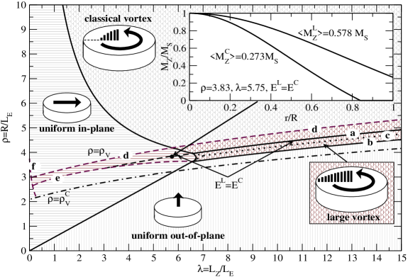
Figure 1: Equilibrium and stability of large magnetic vortex state in circular cylinders of different radii $R$ and thicknesses $L_{Z}$ in soft magnetic material with exchange length $L_{E}$ and saturation magnetization $M_{S}$. Solid lines separate the regions (also having different texture), where different states (uniform in-plane, uniform out-of-plane, classical vortex and large vortex) have the lowest energy. They correspond to particle geometries, where the energy of respective pairs of states is equal. Cylinder geometries, where large magnetic vortex can be metastable, are shown by darker shading. Lettered lines, outlining this stability region, are discussed in the text, they correspond to different modes of vortex stability loss. The line $\rho_{V}^{C}$ shows the radius of classical vortex (which depends only on cylinder’s thickness), computed by Usov and PeschanyUP93 . Inset shows out-of-plane magnetization component distribution $M_{Z}/M_{S}$ as function of reduced radial coordinate $r/R$ in large and classical vortex at a particular geometry, where they both are stable and have the same energy ($E^{L}=E^{C}$).

Potentially, the files allow to extract much more information, but for now, let us focus on the ground state diagram, as it already displays a new simple and fundamental result: there is another magnetic vortex state, which, in tall cylinders ($L_{Z}\gtrsim 6.5$) of certain radii, is, actually, the ground state. At larger cylinder radii the energy of this state becomes equal (shown by the solid line a in Figure) and then larger than the energy of the classical magnetic vortex. At smaller radii it continuously transforms into the state of completely uniform out-of-plane magnetization (solid line b). This expands the region of existence of magnetic vortices to particles of smaller radii and solves a well known paradoxGN04_JAP_PERP ; ML08 that (when the large vortices are not taken into account) the uniform out-of-plane state continues to be the ground state of the cylinder (with energy, smaller than that of classical vortex) with geometries (below the dotted line c and above line b), where it is no longer stable with respect to transformation into magnetic vortex. The line b corresponds to the second order phase transition during which the uniform state loses stability and total Z-component of magnetization starts to deviate from $M_{S}$. The line a corresponds to the first order transition, accompanied by hysteresis, so that the large vortices may exist as metastable in certain region above it, while the classical vortices may exist below this line (they continue to be stable with respect to core expansion in cylinders with radii down to equilibrium classical vortex core radius, shown in Figure as dash-dotted line $\rho_{V}^{C}$).

To confirm the above numerical results and also to fully outline the region of stability of the large magnetic vortices let us now proceed with analytical consideration.

Two interactions, present in any ferromagnet, are the exchange and magnetostatic self-interaction. In continuum approximation, assuming the magnetization texture is simply a function of coordinates $\vec{m}(\vec{r})$, $r=\{X,Y,Z\}$, the exchange energy can be represented as

$$E_{EX}=\frac{CM_{S}}{2}\int\!\!\!\int\!\!\!\int_{V}\sum\limits_{i=X,Y,Z}(\vec{\nabla}m_{i}(\vec{r}))^{2}\,{\mathrm{d}}^{3}\vec{r},$$ (2)

where integration is performed across the volume of the magnet $V$, outside of the magnet $|m|=0$. In the considered case of vortices, larger then the particle radius, the magnetization texture can be described by the following analytical function of complex variable

$$f(t)=\frac{\imath t}{\rho_{V}},$$ (3)

with $\rho_{V}=R_{V}/R>1$ is the normalized vortex core radius $R_{V}$. Since $\rho_{V}>1$, this magnetization texture is all-solitonM10 . That is, contrary to the case of classical magnetic vortex, there is no region in the particle, where magnetization vector lies in the cylinder plane. In this case, the exchange energy can be expressed directly in terms of $f(z)$ as

$$E_{EX}=4CM_{S}\int\!\!\!\int\!\!\!\int_{V}\frac{|f^{\prime}(t)|^{2}}{(1+|f^{\prime}(t)|^{2})^{2}}\,{\mathrm{d}}^{3}\vec{r},$$ (4)

which, after integration, gives

$$e_{EX}^{L}=\frac{4}{\rho^{2}(1+\rho_{V}^{2})},$$ (5)

where the dimensionless energy $e=E/(\mu_{0}\gamma_{B}M_{S}^{2}\pi L_{Z}R^{2})$ and dimensionless particle radius $\rho=R/L_{E}$ were introduced.

To compute the magnetostatic energy let us employ magnetic charges formalism, following from Maxwell’s equations in the static case with no macroscopic currents present. Then, it is possible to express the demagnetizing field via gradient of a scalar potential, which is solution of Poisson’s equations with the volume density of magnetic charge $\Omega=-\mathrm{div}\vec{M}$ on the right hand side. On the boundary of magnetic material this volume density reduces to localized surface density of magnetic charge, equal to the component of magnetization vector, normal to the boundary. In the case of centered large vortex (3) only the surface magnetic charge on the particle face, proportional to out-of-plane component of magnetization $\sigma=M_{z}$ is present. Its energy can be expressed as

$$e_{MS}=\frac{1}{g}\left(w\left(\rho_{V},0\right)-w\left(\rho_{V},g\right)\right),$$ (6)

where the magnetostatic function

$$w(\rho_{v},g)=\!\!\int\limits_{0}^{1}\!\int\limits_{0}^{2\pi}\!\int\limits_{0}^{1}\!\int\limits_{0}^{2\pi}\!\!\frac{\sigma(r_{1},\varphi_{1})\sigma(r_{2},\varphi_{2})r_{1}\,{\mathrm{d}}r_{1}\,{\mathrm{d}}\varphi_{1}r_{2}\,{\mathrm{d}}r_{2}\,{\mathrm{d}}\varphi_{2}}{\sqrt{r_{1}^{2}\!+\!r_{2}^{2}\!-\!2r_{1}r_{2}\cos(\varphi_{1}\!-\!\varphi_{2})\!+\!g^{2}}},$$ (7)

with $r$ and $\varphi$ being dimensionless coordinates on cylinder’s face. For centered vortex (3) the density of face charges does not depend on $\varphi$ and the integral over the angles can be factored out, producing

$$w(\rho_{v},g)=$$ (8)

$$\frac{2}{\pi}\int\limits_{0}^{1}\!\int\limits_{0}^{1}\frac{r_{1}r_{2}(\rho_{V}^{2}-r_{1}^{2})(\rho_{V}^{2}-r_{2}^{2})K(-\frac{4r_{1}r_{2}}{g^{2}+(r1-r2)^{2}})\,{\mathrm{d}}r_{1}\,{\mathrm{d}}r_{2}}{(\rho_{V}^{2}+r_{1}^{2})(\rho_{V}^{2}+r_{2}^{2})\sqrt{g^{2}+(r1-r2)^{2}}},$$ (9)

where $K(k)$ is complete elliptic integral of the first kind. The function $w$ is a nice continuous function and can be differentiated over $\rho_{v}$ under the integral.

To find equilibrium radius of large magnetic vortex it is now sufficient to differentiate the total energy $e_{EX}+e_{MS}$ over $\rho_{V}$ and require that this derivative is equal to 0, which leads to the following transcendental equation

$$-\frac{8g\rho_{v}}{\rho^{2}(1+\rho_{V}^{2})^{2}}+\frac{\partial}{\partial\rho_{V}}\left(w\left(\rho_{V},0\right)-w\left(\rho_{V},g\right)\right)=0.$$ (10)

This equation is hard to solve for $\rho_{V}$. However, it is easy to solve for $\rho$, which gives

$$\rho=\frac{2}{1+\rho_{V}^{2}}\sqrt{\frac{2g\rho_{V}}{\partial_{\rho_{V}}w\left(\rho_{V},0\right)-\partial_{\rho_{V}}w\left(\rho_{V},g\right)}},$$ (11)

allowing to compute the radius of the cylinder $\rho$ in which the large vortex of specified radius $\rho_{V}$ would be at equilibrium. The limit $\rho_{V}\rightarrow\infty$ of this expression immediately recovers the line b in Figure – the boundary at which the large vortices (at larger radii) lose their chirality and become the uniform out-of-plane state (at smaller radii).

The other stability boundary of the large vortex state, line d, can be found in two different ways. One is direct but cumbersome, by considering the transformation between the all-soliton magnetic vortex and the classical one, looking for the particle geometry where the former becomes unstable with respect to transformation into the latter. This can be achieved by considering magnetization distributions, expressed via the complex function

$$w(t,\overline{t})=\left\{\begin{array}[]{ll}f(z)&|f(z)|\leq 1\\ \frac{f(t)}{|f(t)|\sin^{2}\alpha+\cos^{2}\alpha}&|f(z)|>1\end{array}\right..$$ (12)

This function is, in general, not analytical. At $\alpha=0$ it describes all-soliton vortex and at $\alpha=\pi/2$ non-analytical everywhere classical vortex, having a meron part at $|t|>\rho_{V}$. The line d can be obtained as a boundary at which the energy minimum at $\alpha=0$ disappears. Such analysis was indeed performed, however, it turns out (at least to numerical precision) that all-soliton vortices lose stability right at the moment their core boundary touches the particle boundary. Then they immediately transform into classical vortices of much smaller core radius $\rho_{V}^{C}$. Thus, the line d can be found simply by computing the particle radius (11) in the limit $\rho_{V}\rightarrow 1$.

There is another catch that the line b we have just computed becomes unphysical when the aspect ratio of the particle $g=L_{Z}/R$ becomes smaller then approximately $1.81295$. At thinner cylinders the uniform in-plane state becomes the ground state and it becomes necessary to study the transformation of the large vortex state into it. This can be done by considering the uniform tilt of the magnetization in the large vortex, described by the complex function

$$f^{\mathrm{tilt}}(t)=\frac{\imath f(t)\cos(\alpha/2)+\sin(\alpha/2)}{\imath\cos(\alpha/2)+f(t)\sin(\alpha/2)}.$$ (13)

At $\alpha=0$ it is a pure large vortex (3), but, as $\alpha$ increases, it’s magnetization uniformly rotates towards the particle plane. The stability line, then, corresponds to the disappearance of the energy minimum at $\alpha=0$ and can be found by solving the equation

$$\left.\frac{\partial^{2}e^{\mathrm{tilt}}}{\partial\alpha^{2}}\right|_{\alpha=0}=\left.\frac{\partial^{2}e_{EX}^{\mathrm{tilt}}}{\partial\alpha^{2}}+\frac{\partial^{2}e_{MS}^{\mathrm{tilt}}}{\partial\alpha^{2}}\right|_{\alpha=0}=0$$ (14)

at equilibrium $\rho_{V}$. Since the $f^{\mathrm{tilt}}(t)$ is still an analytical function of $t$ the exchange energy $e_{EX}^{\mathrm{tilt}}$ can be directly obtained from (4). The magnetostatic energy, however, now has volume and side surface charge contribution in addition to the energy of face charges. Moreover, there is an interaction between the side and volume charges (their interaction with face charges is canceled by symmetry), which also depend on the polar angle $\varphi$. This makes it necessary to adopt another method of computing magnetostatic energy as angular integrals can’t be directly factored-out. First, let us merge the volume and side charges density together, using Dirac’s delta function $\delta(x)$ to express the side charges localization. Their product (entering the magnetostatic integral) is

$$\left.\frac{\partial^{2}}{\partial\alpha^{2}}\Omega(r_{1},\varphi_{1},\alpha)\Omega(r_{2},\varphi_{2},\alpha)\right|_{\alpha=0}=2\,\omega(r_{1},\varphi_{1})\omega(r_{2},\varphi_{2}),$$ (15)

where

$$\omega(r,\varphi)=-\frac{4r\rho_{v}^{2}\sin\varphi}{(r^{2}+\rho_{V}^{2})^{2}}+\frac{(1-\rho_{V}^{2})\delta(1-r)\sin\varphi}{1+\rho_{V}^{2}}.$$ (16)

The integral of such product of charges can be very efficiently evaluatedGM01 by representing the inverse distance in polar coordinates via Lipshitz internal and then using the Bessel’s summation theorem to factor the angular integral out, which gives

$$\left.\frac{\partial^{2}e_{MS}^{\mathrm{tilt}}}{\partial\alpha^{2}}\right|_{\alpha=0}=\frac{1}{2}\int_{0}^{\infty}\frac{f_{MS}(kg)}{k}\left(\int_{0}^{1}\omega(r,\varphi)J_{1}(kr)r\,{\mathrm{d}}r\right)^{2}\,{\mathrm{d}}k,$$ (17)

where $J_{1}(x)$ is Bessel’s function of the first kind and the delta function is assumed to be right-sided. This integral was evaluated numerically, which is sufficient to solve the transcendental equation (14) and compute the stability line e. Below this line the large vortices, if created, immediately convert into the uniform in-plane state. A confirmation of the consistency of the performed computations is the fact that the line e joins the line b exactly at the critical aspect ratio $g=1.81295$ at which the energies of uniform in-plane and out-of-plane states are equal.

Finally, there is another possibility of vortex conversion into the uniform in-plane state, not captured by the expression (13). At very small thicknesses the vortex may become unstable with respect to lateral shift. The stabilizing force in this case is produced by the side magnetic charges, whose role quickly diminishes as particle becomes thinner. The corresponding stability line f can be found by equating to zero the second derivative in $a$ at $a=0$ of the energy of magnetization distribution, corresponding to the following complex function

$$f^{\mathrm{shift}}(t)=\frac{\imath(z-a)}{\rho_{V}}.$$ (18)

The face charges energy is unchanged in this case, and the balance of forces is established between the exchange (4) and magnetostatic interaction of side charges. The exchange prevails for radii below the stability line f and the particle becomes uniformly magnetized in-plane.

Let us now discuss limitations of the above consideration. In reality there will be a deviation from the assumption of magnetization uniformity across cylinder’s thickness. However, its influence on the phase diagram lines (in the considered range of thicknesses) is negligible, as evidenced by 3-d micromagnetic simulations and experimentScholz2003 . Also, the metastability region of large vortex state comes down to $L_{Z}/L_{E}\sim 0.3$, where magnetization thickness independence is beyond any doubt. Full 3-d models can, however, bring in new effects. At large thicknesses the opposite faces of cylinder become magnetostatically decoupled, so in thicker cut cones (such as commonly produced by lithography), it might be possible to have a metastable large vortex state on smaller face, while having only the small classical-like vortex stable on larger face. Such states can be useful e.g. for readout of stored information, but their existence needs a separate confirmation. Lithographic process may also produce other defects, such as imperfect boundary or local variations of thickness. While large deviations of this kind would produce completely unpredictable magnetic configurations, small random defects usually pin down states across the first order phase transition boundary and make hysteresis loops wider. Experimental points in Fig 14 of Ref. Scholz2003, also indicate that dots with dimensions, supporting large vortices, are experimentally accessible and are not superparamagnetic. The exact lifetime analysis of these states still needs to be performed, but from fundamental point of view they are viable and must be kinetically stable at least at sufficiently low temperatures.

Concluding, it was shown that there is another vortex state in ferromagnetic circular cylinders with vortex core radius, larger than the particle radius. In certain range of particle geometries this large vortex may coexist with classical vortexUP93 , whose core is fully inside the particle. In this region one may have the energies of both classical vortex and large vortex equal (see inset in Figure) while their magnetic moment differs significantly. It should be possible to switch magnetization between these two vortex states (e.g. by applying current through the particle). Moreover, because these states can be continuously transformed into one another without formation of Bloch points or other topological singularities and are otherwise very similar to each other, such switching can be expected to be very fast.

Acknowledgments. The distributed computation under the umbrella of Magnetism@home project was made possible thanks to participation of numerous volunteers, whose help is gratefully acknowledged. I’d like to thank Alexander E. Filippov for reading the manuscript and many valuable suggestions.

References

- (1) N. A. Usov and S. E. Peschany, J. Magn. Magn. Mater. 118, L290 (1993)
- (2) T. Shinjo, T. Okuno, R. Hassdorf, K. Shigeto, and T. Ono, Science 289, 930 (2000)
- (3) B. Van Waeyenberge, A. Puzic, H. Stoll, K. W. Chou, T. Tyliszczak, R. Hertel, M. Fahnle, H. Bruckl, K. Rott, G. Reiss, I. Neudecker, D. Weiss, C. H. Back, and G. Schutz, Nature 444, 461 (2006), ISSN 0028-0836
- (4) R. Antos and Y. Otani, Phys. Rev. B 80, 140404 (2009)
- (5) M. Kammerer, M. Weigand, M. Curcic, M. Noske, M. Sproll, A. Vansteenkiste, B. Van Waeyenberge, H. Stoll, G. Woltersdorf, C. H. Back, and G. Schuetz, Nat Commun 2, 279 (2011)
- (6) R. Hertel, S. Gliga, M. Fähnle, and C. M. Schneider, Phys. Rev. Lett. 98, 117201 (Mar 2007)
- (7) K.-S. Lee, K. Y. Guslienko, J.-Y. Lee, and S.-K. Kim, Phys. Rev. B 76, 174410 (2007)
- (8) K. Y. Guslienko, K.-S. Lee, and S.-K. Kim, Phys. Rev. Lett. 100, 027203 (2008)
- (9) H. W. Schumacher, C. Chappert, R. C. Sousa, P. P. Freitas, and J. Miltat, Phys. Rev. Lett. 90, 017204 (2003)
- (10) S. Choi, K.-S. Lee, K. Y. Guslienko, and S.-K. Kim, Phys. Rev. Lett. 98, 087205 (2007)
- (11) K. L. Metlov, Phys. Rev. Lett. 105, 107201 (2010)
- (12) K. L. Metlov and K. Y. Guslienko, Phys. Rev. B 70, 052406 (2004)
- (13) P. Visscher and D. Apalkov, “Simple recursive cartesian implementation of fast multipole algorithm,” (2003), preprint at bama.ua.edu/ visscher/mumag/cart.pdf
- (14) A. Aharoni, Introduction to the theory of ferromagnetism (Oxford University Press, Oxford, 1996) ISBN 0198517912
- (15) K. Y. Guslienko and V. Novosad, J. Appl. Phys. 96, 4451 (2004)
- (16) K. L. Metlov and Y. P. Lee, Appl. Phys. Lett. 92, 112506 (2008)
- (17) K. Y. Guslienko and K. L. Metlov, Phys. Rev. B 63, 100403R (2001)
- (18) W. Scholz, K. Guslienko, V. Novosad, D. Suess, T. Schrefl, R. Chantrell, and J. Fidler, Journal of Magnetism and Magnetic Materials 266, 155 (2003), ISSN 0304-8853