Decoupling absorption and continuum variability in the Seyfert 2 NGC 4507

Abstract

We present the results of the Suzaku observation of the Seyfert 2 galaxy NGC 4507. This source is one of the X-ray brightest Compton-thin Seyfert 2s and a candidate for a variable absorber. Suzaku  caught NGC 4507 in a highly absorbed state characterised by a high column density ($N_{\mbox{\scriptsize H}}\sim 8\times 10^{23}$ cm^-2), a strong reflected component ($R\sim 1.9$) and a high equivalent width $\mbox{Fe~{}K}\alpha$ emission line ($EW\sim 500$ eV). The $\mbox{Fe~{}K}\alpha$ emission line is unresolved at the resolution of the Suzaku CCDs ($\sigma<30$ eV or $FWHM<3000$ km s^-1) and most likely originates in a distant absorber. The Fe K$\beta$  emission line is also clearly detected and its intensity is marginally higher than the theoretical value for low ionisation Fe. A comparison with previous observations performed with XMM-Newton and BeppoSAX reveals that the X-ray spectral curvature changes on a timescale of a few months. We analysed all these historical observations, with standard models as well as with a most recent model for a toroidal reprocessor and found that the main driver of the observed 2–10 keV spectral variability is a change of the line-of-sight obscuration, varying from $\sim 4\times 10^{23}$ cm^-2 to $\sim 9\times 10^{23}$ cm^-2. The primary continuum is also variable, although its photon index does not appear to vary, while the $\mbox{Fe~{}K}\alpha$ line and reflection component are consistent with being constant across the observations. This suggests the presence of a rather constant reprocessor and that the observed line of sight $N_{\mbox{\scriptsize H}}$ variability is either due to a certain degree of clumpiness of the putative torus or due to the presence of a second clumpy absorber.

1 Introduction

The main ingredient of the widely accepted Unified Model (Antonucci, 1993) of Active Galactic Nuclei (AGN) is the presence along the line of sight towards type 2 (or obscured) AGN of optically-thick material covering a wide solid angle. This absorber was thought to be rather uniform and distributed in a toroidal geometry, which is located at a pc scale distance from the nuclear region (Urry & Padovani, 1995) or in the form of a bi-conical outflow (Elvis, 2000). Although this model has been to first order confirmed, it is now clear that this is only a simple scenario, which does not hold for all AGN (Bianchi et al. 2012; Turner et al. 2012; Turner & Miller 2009). In particular X-ray observations of nearby and bright AGN unveiled the co-existence of multiple absorbers/reflecting mirrors in the central regions, suggesting that the absorbers could be located at different scales (from within few tens of gravitational radii from the central nucleus to outside the pc-scale torus) and could be in part inhomogeneous (Risaliti et al. 2002; Elvis et al. 2004). Our view of the inner structure of AGN has been also modified by the recent finding of hard excesses in type 1 AGN, which can be modelled with the presence of a Compton-thick gas in the line-of-sight (PDS 456, Reeves et al. 2009, 1H 0419-577, Turner et al. 2009 and Tatum et al. 2012).

The variability of the column density of the X-ray absorbing gas ($N_{\mbox{\scriptsize H}}$) observed in a large number of AGN revealed that a significant fraction of the absorbing medium must be clumpy. The time-scales of these $N_{\rm H}$ variations, which can be directly linked to the size and distance of the absorbing clouds, also provided valuable constraints on the size and location of this obscuring material from the central accreting black hole (see Risaliti et al. 2002). Rapid $N_{\rm H}$ variations have been discovered on time-scales from a few days down to a few hours for a limited but still increasing number of obscured or type 2 AGN: NGC 1365 (Risaliti et al. 2005, 2007, 2009; Maiolino et al. 2010), NGC 4388 (Elvis et al. 2004), NGC 4151 (Puccetti et al. 2007), NGC 7582 (Piconcelli et al. 2007; Bianchi et al. 2009; Turner et al. 2000) and UCC 4203 (Risaliti et al., 2010). Some of these extreme variations are effectively occultation events where the column density of the absorber changes from Compton-thin ($N_{\mbox{\scriptsize H}}<10^{24}$ cm^-2) to Compton-thick ($N_{\mbox{\scriptsize H}}>10^{24}$ cm^-2). These $N_{\rm H}$ variations unveiled that a significant fraction of such absorbing clouds must be located very close to the nuclear X-ray source and, more specifically, within the broad line region (BLR).

However this picture is proven only for those few objects, which show extreme and rapid $N_{H}$ variations. On longer time-scales (from months to years) $N_{\rm H}$ variability is a common property in local bright Seyfert 2 galaxies (Risaliti et al. 2002). Due to the complexity of the measurements, when a change in the spectral shape is found it is hard to distinguish between $N_{\mbox{\scriptsize H}}$ and photon index variations. The main open question for some of the detected variations is whether the spectral changes are indeed due to a variable circum-nuclear absorber or are due to variability of the intrinsic emission. In order to remove this degeneracy, high sensitivity and wide spectral coverage (to determine the continuum component) are needed. Variability of the X-ray absorbers is a common property of AGN. Indeed, in type 1 AGN (see Turner & Miller 2009; Bianchi et al. 2012) most of the observed spectral variability can be described with changes in the covering factors and ionisation states of the inner absorbers (NGC 4051, Miller et al. 2010; MCG-06-30-15, Miller et al. 2008; Mrk766, Miller et al. 2007; Turner et al. 2007; PDS 456, Behar et al. 2010). Furthermore, even if rare, occultation events have been detected in type 1 AGN: Mrk 766 (Risaliti et al. 2011) and NGC 3516 (Turner et al., 2008), supporting the overall picture.

The hypothesis of a clumpy structure for the absorbing “torus” has been recently introduced in several theoretical models (Nenkova et al. 2002, 2008; Elitzur & Shlosman 2006; Elitzur 2012 and reference therein), where the torus consists of several distinct clouds, distributed in a soft-edge torus. These models were originally based on infrared observations (Jaffe et al., 2004; Poncelet et al., 2006), showing an apparent similarity between the IR emission of type 1 and type 2 AGN (Lutz et al., 2004; Horst et al., 2006), but are now strongly supported by the short-term changes of the $N_{\rm H}$ of the X-ray absorbers. As discussed by Elitzur (2012), for a “soft-edged” toroidal distribution of clouds, the classification of type 1 and type 2 does not depend solely on the viewing angle; although the probability of a “unobscured view” of the AGN decreases when the line-of-sight is far from the axis, it is non zero. Furthermore, this model naturally accounts for $N_{\rm H}$ variability and in particular for occultations events due to the transition of a single cloud.

NGC 4507 is one of the X-ray brightest ($F_{(2-10~{}\mathrm{keV})}\sim 0.6-1.3\times 10^{-11}$ erg cm^-2 s^-1), and nearby ($z=0.0118$) Seyfert 2 galaxies, with an estimated unabsorbed luminosity of $3.7\times 10^{43}$ erg s^-1(Comastri et al. 1998). It has been observed with all the major X-ray observatories; Einstein (Kriss et al. 1980); Ginga (Awaki et al. 1991); BeppoSAX (Risaliti, 2002; Dadina, 2007); ASCA (Turner et al., 1997; Comastri et al., 1998); XMM-Newton; Chandra  (Matt et al., 2004) and Rossi X-Ray Timing Explorer (RXTE; Rivers et al. 2011). NGC 4507  is one of the brightest Seyfert 2s detected above 10 keV with the both BAT detector on board Swift and INTEGRAL. It is part of the 58 months BAT catalogue (Tueller et al. 2010; Baumgartner et al. 2012 ApJS submitted) and of the INTEGRAL AGN catalogue ($F_{(20-100~{}\mathrm{keV})}\sim 2\times 10^{-10}$erg cm^-2 s^-1; Beckmann et al. 2009; Malizia et al. 2009; Bassani et al. 2006). NGC 4507 was also detected in the soft gamma-ray band with the OSSE experiment on board the Compton Gamma Ray Observatory (Bassani et al., 1995).

All of these X-ray observations revealed a hard X-ray spectrum typical of a Compton-thin Seyfert 2: an X-ray continuum characterised by heavy obscuration and a strong Fe K$\alpha$ line at 6.4 keV. The average measured column density is $N_{\rm H}\sim 6\times$10²³ cm^-2 (Risaliti, 2002). A reflection component with a reflection fraction ranging from 0.7 to 2.0 (Risaliti, 2002; Dadina, 2007) was measured with the BeppoSAX observations, while the high energy cut-off could not be constrained. A similar result has been obtained with the INTEGRAL IBIS/ISGRI data ($R=0.6^{+1.5}_{-0.5}$; Beckmann et al. 2009).

The soft X-ray spectrum is also typical of a Compton-thin Seyfert 2, with several emission lines from 0.6–3 keV range, due to ionised elements from O to Si, which require the presence of at least two photoionised media or a single stratified medium (Matt et al. 2004). A comparison between the observations performed with BeppoSAX and ASCA   showed long-term $N_{\rm H}$ variability, which changes by a factor of 2, and also some possible variability of the intrinsic continuum (Risaliti et al. 2002; Risaliti 2002). Altogether the emerging picture for NGC 4507 is of a complex and highly variable absorber, as seen in other bright Compton-thin Seyfert 2s. At least two absorbing systems are present: a Compton-thick reprocessor, responsible for the Fe K$\alpha$ line at 6.4 keV plus the strong Compton reflected component detected with BeppoSAX and RXTE (Rivers et al. 2011), and a variable Compton-thin absorber. A Chandra observation also provided a detection (at 99% significance) of a Fe xxv absorption line (at $\sim 6.7$ keV), which suggested the presence of an ionised absorber (Matt et al., 2004).

Here, we present the results of a Suzaku observation (of net exposure $\sim 90$ ks) of NGC 4507 and a comparison with previous X-ray observations of this AGN, which shows that below 10 keV NGC4507 alternates from being in a transmission to a “reflection” dominated state. The Suzaku observation has been already presented in the statistical analysis of 88 Seyfert 2 galaxies observed by Suzaku (Fukazawa et al., 2011), investigating the properties of the Fe K complex versus the amount of absorption and luminosity of the sources. Fukazawa et al. 2011 report both the presence of a high column density absorber as well as a strong Fe K line complex ($EW=600\pm 30$ eV). Here we present a more detailed analysis of the same observation, where we investigate the Fe K line complex allowing not only the $\mbox{Fe~{}K}\alpha$  but also the Fe K$\beta$  line parameters ($E$, $\sigma$ and $I$) to vary as well as a comparison with the previous X-ray observations. Finally, we also tested a new model for the toroidal reprocessor (Murphy & Yaqoob, 2009).

The paper is structured as follows. The observation and data reduction are summarised in § 2. In § 3 we present the modelling of the broad-band spectrum obtained with Suzaku, aimed to assess the nature of the X-ray absorber, the amount of reflection and the iron K emission line. In § 4 we then compare the Suzaku  with the previous XMM-Newton and BeppoSAX observations. Discussion and conclusions follow in § 5. Throughout this paper, a concordance cosmology with H${}_{0}=71$ km s^-1 Mpc^-1, $\Omega_{\Lambda}$=0.73, and $\Omega_{m}$=0.27 (Spergel et al., 2003) is adopted.

2 Observations and data reduction

2.1 Suzaku

A Suzaku (Mitsuda et al., 2007) observation of NGC 4507 was performed on 20th December 2007 for a total exposure time of about 103 ksec (over a total duration of $\sim 178$ ksec); a summary of the observations is shown in Table 1. Suzaku  carries on board four co-aligned telescopes each with an X-ray CCD camera (X-ray Imaging Spectrometer; XIS Koyama et al., 2007) at the focal plane, and a non imaging hard X-ray detector (HXD-PIN; Takahashi et al. 2007). Three XIS (XIS0, XIS2 and XIS3) are front illuminated (FI), while the XIS1 is back illuminated; the latter has an enhanced response in the soft X-ray band but lower effective area at 6 keV than the XIS-FI. At the time of this observation only two of the XIS-FI were still operating, namely the XIS0 and XIS3. All together the XIS and the HXD PIN instruments cover the 0.5–10 keV and 14–70 keV bands respectively. The cleaned XIS event files obtained from version 2 Suzaku pipeline processing were processed using HEASOFT (version v6.6.3) and the Suzaku reduction and analysis packages applying the standard screening for the passage through the South Atlantic Anomaly (SAA), elevation angles and cut-off rigidity. The XIS data were selected in $3\times 3$ and $5\times 5$ editmodes using only good events with grades 0, 2, 3, 4, 6 and filtering the hot and flickering pixels with the script sisclean. The net exposure times are $87.7$ ksec for each of the XIS and $92.9$ ksec for the HXD-PIN.

The XIS source spectra were extracted from a circular region of 2.6^′ radius centered on the source, while background spectra were extracted from two circular regions of 2.6^′ radius offset from the source and the Fe 55 calibration sources, which are in two corners of CCDs. The XIS response (rmfs) and ancillary response (arfs) files were produced, using the latest calibration files available, with the ftools tasks xisrmfgen and xissimarfgen respectively. The spectra from the two FI CDDs (XIS 0 and XIS 3) were combined in a single source spectrum (hereafter XIS–FI) after checking for consistency, while the BI (the XIS1) spectrum was kept separate and fitted simultaneously. The net 0.6–10 keV count rates are: $(0.128\pm 0.001)$ counts s^-1, $(0.131\pm 0.001)$ counts s^-1, $(0.128\pm 0.001)$ counts s^-1 for the XIS 0, XIS3 and XIS1 respectively. Data were included from 0.6–10 keV for the XIS–FI and 0.6–8.5 keV for the XIS1 chip; the difference on the upper boundary for the XIS1 spectra is because this CCD is optimised for the soft X-ray band. We also excluded the data in the 1.6–1.9 keV energy range due to calibration uncertainties. The XIS FI (BI) source spectra were binned to 1024 channels and then to a minimum of 100 (50) counts per bin, and $\chi^{2}$ statistics have been used.

The HXD-PIN data were reduced following the latest Suzaku data reduction guide (the ABC guide Version 4.0), and using the rev2 data, which include all 4 cluster units. The HXD-PIN instrument team provides the background event file (known as the “tuned” background), which accounts for the instrumental Non X-ray Background (NXB; Kokubun et al., 2007). The systematic uncertainty of this “tuned” background model is believed to be $\pm$1.3% (at the 1$\sigma$ level for a net 20 ks exposure). We extracted the source and background spectra using the same common good time interval, and corrected the source spectrum for the detector dead time. The net exposure time after screening was 92.9 ks. We simulated a spectrum for the cosmic X-ray background counts adopting the form of Boldt (1987) and Gruber et al. (1999) and the response matrix for the diffuse emission; the resulting spectrum was then added to the instrumental one.

NGC 4507 is detected up to 70 keV at a level of 23.6% above the background corresponding to a signal-to-noise ratio $S/N\sim 50$. The net count rate in the 14–70 keV band is $0.122\pm 0.002$ counts s^-1 ($\sim 11300$ net counts). For the spectral analysis the source spectrum of NGC 4507 was rebinned in order to have a signal-to-noise ratio of 10 in each energy bin. A first estimate of the 14–70 keV flux was derived assuming a single absorbed power-law ($\Gamma=1.8\pm 0.3$) model. The 14–70 keV flux is about $\sim 9.2\times 10^{-11}$erg cm^-2 s^-1 and the extrapolated flux in the Swift  band (14–195 keV) is $\sim 1.8\times 10^{-10}$erg cm^-2 s^-1, comparable to the flux reported in the BAT 58 months catalog ($\sim 1.9\times 10^{-10}$erg cm^-2 s^-1, Baumgartner et al. 2012 ApJS submitted).

2.2 XMM-Newton

XMM-Newton observed NGC 4507 on the 4th January 2001 (see Table 1) with a total exposure time of about 46.2 ksec. This observation was presented by Matt et al. (2004). Since we are mainly interested in a comparison with the Suzaku observation and since a detailed analysis has been already published, we focused only on the EPIC-pn data. The EPIC-pn camera had the medium filter applied and was operating in Full Frame Window mode. The XMM-Newton data were processed and cleaned using the Science Analysis Software (SAS version 10.0.2) and analysed using standard software packages and the most recent calibrations. In order to define the threshold to filter for high-background time intervals, we extracted the 10–12 keV light curves and filtered out the data when the light curve is 2$\sigma$ above its mean. This screening yields net exposure time (which also includes the dead-time correction) of $\sim 32$ ksec. The EPIC pn source spectrum was extracted using a circular region of $35^{\prime\prime}$ and background data were extracted using two circular regions with a radius of $30^{\prime\prime}$ each. Response matrices and ancillary response files at the source position were created using the SAS tasks arfgen and rmfgen. The source spectrum was then binned to have at least 50 counts in each energy bin.

2.3 The Swift-BAT

The Swift-BAT spectrum and the latest calibration response file (the diagonal matrix: diagonal.rsp) were obtained from the 58-month survey archive; the data reduction procedure of the eight-channel spectrum is described in Tueller et al. (2010) and Baumgartner et al. (2012 ApJS submitted). The net count rate in the 14–195 keV band is $(2.69\pm 0.05)\times 10^{-3}$ counts s^-1 (corresponding to $F_{14-195\,\mathrm{keV}}\sim 1.9\times 10^{-10}$erg cm^-2 s^-1).

Table 1: Summary of the observations used: Observatory, Epoch, Instrument, and Net exposure times. The net exposure times are after the screening of the cleaned event files.

Mission	DATE	Instrument	T(net) (ks)
Suzaku	2007-12-20	XIS	87.7
Suzaku	2007-12-20	HXD-PIN	92.7
XMM-Newton	2001-01-04	EPIC-pn	32.3
BeppoSAX 1	1997-12-26	MECS	49.79
BeppoSAX 1	1997-12-26	PDS	26.97
BeppoSAX 2	1998-07-02	MECS	31.41
BeppoSAX 2	1998-07-02	PDS	16.95
BeppoSAX 3	1999-01-13	MECS	41.33
BeppoSAX 3	1999-01-13	PDS	20.08

3 Spectral analysis

All the models were fit to the data using standard software packages (xspec ver. 12.7.0 Arnaud 1996) and including Galactic absorption ($N_{\rm{H,Gal}}=7.23\times 10^{20}$cm^-2; Dickey & Lockman 1990). In the following, unless otherwise stated, fit parameters are quoted in the rest frame of the source and errors are at the 90% confidence level for one interesting parameter ($\Delta\chi^{2}=2.71$).

3.1 The 0.6–150 keV continuum

For the analysis we fitted simultaneously the Suzaku spectra from the XIS-FI (0.6–10 keV), the XIS1(0.6–8.5 keV) HXD-PIN (14–70 keV) and the Swift-BAT spectrum (14–150 keV). We set the cross-normalization factor between the HXD and the XIS-FI spectra to 1.16, as recommended for XIS nominal observation processed after 2008 July (Manabu et al. 2007; Maeda et al. 2008), while we left the cross-normalisation with the Swift-BAT spectrum free to vary.

We initially tested the best-fit continuum model presented in Matt et al. (2004) for the XMM-Newton  data, which was of the mathematical form: $F(E)=\mathrm{wabs}\times(\rm{zwabs}\times\mathrm{pow1}+\mathrm{pexrav}+\mathrm{pow2)}$, where pow1 is the absorbed power-law, pexrav is the xspec model for a Compton-reflected component (Magdziarz & Zdziarski 1995), pow2 is the soft scattered power-law continuum, which is absorbed only by the local Galactic absorber (wabs) and zwabs is the intrinsic absorber. For the pexrav component we allowed only its normalisation to vary, while we fixed the high energy cutoff to 200 keV, the amount of reflection $R=\Omega/2\pi=1$ and the inclination angle i to 30^∘, as adopted by the previous work on the XMM-Newton data.

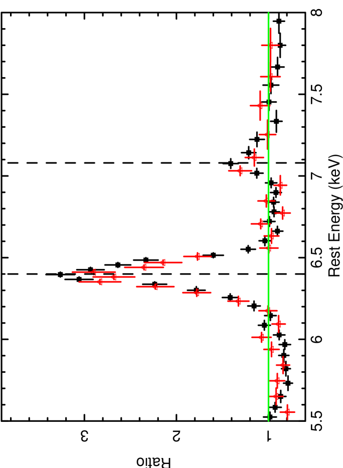
Figure 1: Data/model ratio between the XIS data (XIS-FI, black filled squares in the electronic version; XIS-BI red open triangles in the electronic version) and the continuum model, showing the iron line profile. The two vertical dashed lines correspond to the rest-frame energies of the Fe K$\alpha$ and K$\beta$ emission lines at 6.4 keV and 7.06 keV respectively.

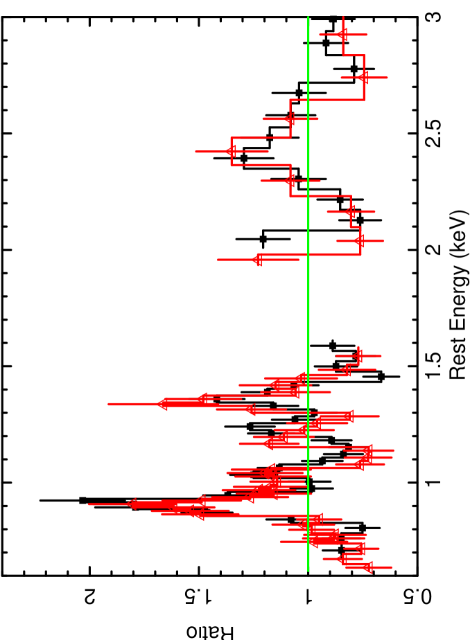
Figure 2: Data/model ratio between the XIS data (XIS-FI, black filled squares in the electronic version; XIS-BI red open triangles in the electronic version) and the continuum model (see § 3.1), showing the soft X-ray lines.

As shown in Fig. 1 the residuals to our baseline continuum model at the energy of the Fe K band clearly reveal the presence of a strong narrow core at the expected energy of the Fe K$\alpha$ ($6.4$ keV), as well as a strong Fe K$\beta$ ($\sim 7.06$ keV). We then included two narrow Gaussian lines to account for Fe K$\alpha$ and K$\beta$ emission lines (see §3.2). Initially we fixed the energy of the Fe K$\beta$ emission line to 7.06 keV, we tied its width to the width of the Fe K$\alpha$ emission line and its normalisation to be 13.5% of the Fe K$\alpha$ emission line (Palmeri et al. 2003). The inclusion of the lines improves the fit by $\Delta\chi^{2}=1511$ for 3 degrees of freedom ($\chi^{2}/\mbox{d.o.f.}$  =723.7/384); statistically the fit is still unacceptable, with most of the remaining residuals being at $E<2$ keV. Following the results of previous X-ray studies of NGC 4507, which showed a remarkably steep X-ray emission below 2 keV accompanied by several soft X-ray emission lines (Matt et al. 2004), we then allowed the scattered component (pow2) to have a different photon index ($\Gamma$; see Table 4) with respect to the primary power law and we added several narrow Gaussian emission lines, which even at the Suzaku CCD resolution are clearly visible (see Fig. 2).

Table 2: Summary of the strongest soft-X-ray emission lines as detected in the Suzaku spectra. The energies of the lines are quoted in the rest frame. Fluxes and possible identifications are reported in column 2 and 3. The observed EW are reported in column 4 and they are calculated against the total observed continuum at their respective energies. In column 5 the improvement of fit is shown with respect to the continuum model; the value for the model with no soft X-ray lines is $\chi^{2}/\mbox{d.o.f.}\ =723.7/384$. Finally in column 6 we report the lab energy for the detected lines.

Energy	Flux	ID	EW	$\Delta\chi^{2}$	ELab
(keV)	($10^{-6}$ph cm-2 s-1)		(eV)		(keV)
(1)	(2)	(3)	(4)	(5)	(6)
0.90${}^{+0.01}_{-0.01}$	28.6${}^{+3.3}_{-3.3}$	Ne ix He-$\alpha$	107${}^{+12}_{-12}$	164.2	0.905(f); 0.915(i);0.922 (r)
1.03${}^{+0.01}_{-0.01}$	7.8${}^{+1.9}_{-1.9}$	Ne x  Ly$\alpha$	46${}^{+11}_{-11}$	21.5	1.022
1.22 ${}^{+0.01}_{-0.01}$	4.6${}^{+1.3}_{-1.3}$	Ne x Ly$\beta$	47${}^{+13}_{-13}$	20.8	1.211 (r)
1.36${}^{+0.01}_{-0.01}$	5.5${}^{+1.1}_{-1.1}$	Mg xi He$\alpha$	76${}^{+15}_{-15}$	69.4	1.331(f); 1.343(i); 1.352 (r)
2.41${}^{+0.03}_{-0.05}$	2.0${}^{+0.9}_{-0.9}$	S xiv K$\alpha$	62${}^{+27}_{-27}$	12.5	2.411
3.70${}^{+0.03}_{-0.03}$	2.1${}^{+0.8}_{-0.8}$	Ca K$\alpha$	58${}^{+20}_{-22}$	19.3	3.69

We detected 6 strong soft X-ray emission lines (from Ne, Mg and S; see Table 2) and although relatively simple, this model already provides a good fit ($\chi^{2}/\mbox{d.o.f.}$ = 416.0/372). However, we note that the soft power-law component is unusually steep ($\Gamma=3.8\pm 0.2$). The steep photon index could be due to the presence of other weak emission lines, which are unresolved at the XIS-CCD resolution and could be related either to the photoionised emitters responsible for the strongest emission lines as seen in Compton-thin Seyfert galaxies (Bianchi et al., 2006; Guainazzi & Bianchi, 2007) or to the presence of additional emission from a collisionally-ionised diffuse gas. Although we investigated different physical scenarios (see §3.2), we note that the different models tested for the soft X-ray emission did not strongly affect the results of the hard X-ray energy band.

3.2 The soft X-ray emission

Although our primary aim is the analysis of the hard X-ray emission, we investigated both photoionised and collisionally ionised plasmas as sources for the soft X-ray emission lines; to this end we fitted the 0.6–150 keV spectra replacing in turn the Gaussian emission lines with either an additional thermal component (mekal model in xspec, Mewe et al. 1985) or a grid of photoionised emission model generated by xstar (Kallman et al., 2004), which assumes a $\Gamma\sim 2$ illuminating continuum and a turbulence velocity of $\sigma_{\rm{v}}=100$ km/s.

We found that neither a single photoionised emission model or a thermal component provide an acceptable the fit ($\chi^{2}/\mbox{d.o.f.}$ =592.3/382 and $\chi^{2}/\mbox{d.o.f.}$ = 584.7/382 for the xstar and mekal component with respect to the model with no soft X-ray lines $\chi^{2}/\mbox{d.o.f.}$ =723.7/384, respectively), and strong residuals are present below 2 keV; furthermore, for both these models we found a steep $\Gamma$ for the the soft power-law component ($\Gamma=3.2\pm 0.2$). Thus we tested for the soft X-ray emission a composite model consisting of: a collisionally ionised emitter, a photoionised plasma and a soft power-law component. We found that this model is now a better representation of the observed emission ($\chi^{2}/\mbox{d.o.f.}$ =510.1/380). The photoionised emitter has an ionisation parameter of log$\xi=1.96$${}^{+0.11}_{-0.07}$ erg cm s^-1, while the thermal component has a temperature of $kT=0.75$ ${}^{+0.06}_{-0.05}$ keV. This model gives a total observed (i.e. corrected only for the Galactic absorption) 0.5–2 keV flux of $\sim 4.8\times 10^{-13}$erg cm^-2 s^-1; in this energy range the relative contribution of the collisionally and photoionised emitters are $F_{0.5-2}^{\mathrm{COLL}}\sim 9.7\times 10^{-14}$erg cm^-2 s^-1  and $F_{0.5-2}^{\mathrm{PHOT}}\sim 1.3\times 10^{-13}$erg cm^-2 s^-1 respectively. We note that the limited spectral resolution of the CCD spectra prevents us from deriving definitive conclusion on the relative importance of these two emission components, furthermore the photon index is still relatively steep $\Gamma=3.0\pm 0.3$, suggesting that there is still a possible contribution from unresolved emission lines or a collisionally ionised emission (e. g. a thermal component).
Recently we obtained a deep ($\sim 130$ ks) XMM-Newton-RGS observation of NGC 4507, which provided the best soft X-ray spectrum so far for NGC 4507. The properties of the soft X-ray emission are discussed in more detail in a companion paper describing the XMM-Newton-EPIC and XMM-Newton-RGS data (Marinucci et al. 2012b, Wang et al. private communication). Briefly the RGS data unveiled that the soft X-ray emission is indeed dominated by emission lines, and that cannot be explained with a single photoionised or thermal component. We stress again that the different models tested for the soft X-ray emission did not strongly affect the results of the hard X-ray emission, which is our primary focus in this paper.

3.3 The Fe K emission line complex and the high energy spectrum

We then considered the hard X-ray emission of NGC 4507  using for the soft X-ray emission the simple phenomenological model of a scattered power-law component and 6 Gaussian emission lines. The spectrum was then parametrized with a model of the form: $F(E)=\mathrm{wabs}\times(\rm{zwabs}\times\mathrm{pow1}+\mathrm{pexrav}+\mathrm{Fe\;K}\alpha+\mathrm{Fe\;}K\beta+\mathrm{pow2+6\;\mathrm{GA}_{\mathrm{em}}})$, where the ratio of $\mbox{Fe~{}K}\alpha$  and Fe K$\beta$  intensities was initially fixed at 13.5% and GA_em are the soft X-ray emission lines. As previously described, the photon index of the scattered power-law component (pow2) was left free to vary independently from the primary power-law component (pow1). This model provides a good description of the continuum ($\chi^{2}/\mbox{d.o.f.}$ = 416.0/372); an intrinsic column density of $N_{\mathrm{H}}=(8.4\pm 0.5)\times 10^{23}$ cm^-2  is required, the photon index of the primary absorbed power law is $\Gamma=1.83\pm 0.04$ and the intensity of neutral reflection component is $N_{\mathrm{PEXRAV}}=(1.2\pm 0.1)\times 10^{-2}$ photons cm^-2s^-1 (corresponding to $R\sim 1.6$).

Taking into account the high statistics of the present data and the strength of both the Fe K lines, we then left free to vary the centroid energy and intensity of the Fe K$\beta$ line and we found a statistically similar best-fit ($\chi^{2}/\mbox{d.o.f.}$ =409.5/370). For the $\mbox{Fe~{}K}\alpha$  line core we obtained $E=6.408$${}^{+0.005}_{-0.004}$ keV, $\sigma=35\pm 10$ eV (corresponding to a $FWHM=3860\pm 1100$ km s^-1) and $EW=490\pm 30$ eV (with respect to the observed continuum). For the corresponding Fe K$\beta$ we obtained a centroid energy of $E=7.07\pm 0.02$ keV and $I_{\mathrm{FeK\beta}}=9.50^{+1.79}_{-1.77}\times 10^{-6}$photons cm^-2s^-1, which corresponds to a $I_{\mathrm{Fe\;K\alpha}}/I_{\mathrm{Fe\;K\beta}}$ ratio to about $\sim 17$%. We also checked the accuracy of the energy centroids and line widths using the ⁵⁵Fe calibration sources located on two corners of each of the XIS chips, which produce lines from Mn K$\alpha$ (K$\alpha 1$ and K$\alpha 2$ at 5.899 keV and 5.888 keV respectively). From measuring the lines in the calibration source, we find no major energy shift or residual broadening ($E=5.903\pm 0.003$ keV, $\sigma<15$ eV). Thus the apparent broadening of the $\mbox{Fe~{}K}\alpha$  emission line is not due to calibration uncertainties, however, upon the inclusion of a possible Compton shoulder the $\mbox{Fe~{}K}\alpha$  is unresolved (see below and §4.1).

The parameters derived for the Fe K line complex are similar to the values reported in Fukazawa et al. (2011); we note however that in our modelling the energy centroids and normalisations of all the lines are left free to vary. In the upper panel of Fig. 3 we show the 68%, 90%, and 99% confidence contours of the narrow Fe K$\beta$ centroid energy versus the centroid energy of the $\mbox{Fe~{}K}\alpha$, while in the lower panel we show the corresponding contours for the line intensities. We note that contamination to the Fe K$\beta$ from a possible Fe xxvi ($E=6.97$ keV) is negligible, indeed as can be seen in Fig. 3 (upper panel) the contours of the energy centroid of the Fe K$\beta$ are fairly symmetric and not elongated toward lower energies. Although the ratio of Fe K$\beta$ and $\mbox{Fe~{}K}\alpha$  intensities is consistent within the errors (at 99%, see Fig. 3, lower panel) with the 13.5% value, as expected for low ionisation Fe (Palmeri et al., 2003), it is marginally higher than the theoretical value for low ionisation Fe; such a high value of the Fe K$\beta$/$\mbox{Fe~{}K}\alpha$  could be indicative that the Fe ionisation state could be as high as Fe ix. In particular Palmeri et al. (2003) showed that while for Fe i both theoretical and experimental values of this ratio lie in the 12–13.5% range, for higher ionisation states this ratio can be higher and for Fe ix it can be as high as 17%.

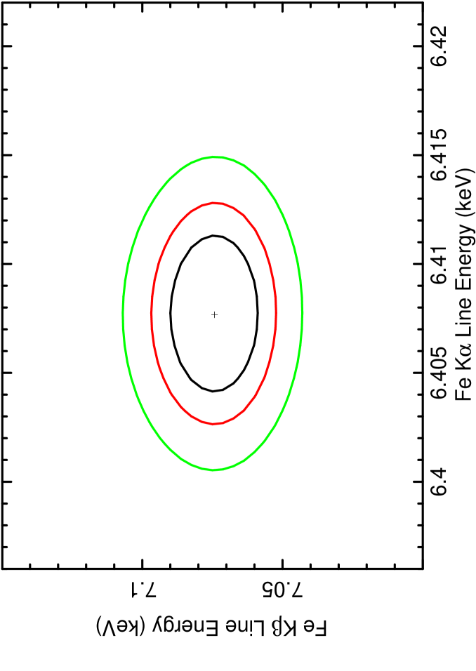
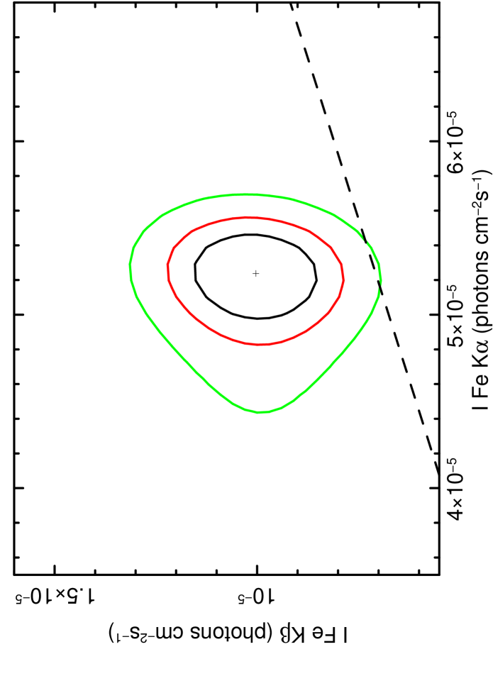
Figure 3: Upper panel: 68%, 90%, and 99% confidence contours of energy centroid of the $\mbox{Fe~{}K}\alpha$ versus the Fe K$\beta$  emission lines (rest frame). Lower panel: 68%, 90%, and 99% confidence contours of the intensity of the $\mbox{Fe~{}K}\alpha$  versus the Fe K$\beta$ emission line; the dashed line corresponds to the Fe K$\beta$/$\mbox{Fe~{}K}\alpha$  line ratio of 0.135.

We note that the parameters of the continuum (see Table 4) and in particular of the reflection component are all well constrained. In Fig. 4, we show the confidence contours between the normalisation of the reflection component and the intrinsic photon index ($\Gamma$), obtained allowing the cross normalisation factor of the HXD over the XIS-FI spectrum to vary. The best fit value of the intensity of the neutral reflection component is $N_{\mathrm{PEXRAV}}=1.2\pm 0.1\times 10^{-2}$ photons cm^-2 s^-1, which corresponds to $R=1.9\pm 0.2$ ; we note that this component dominates the spectrum below $\sim 7$ keV (see Fig. 5).

We found also evidence for the $\mbox{Fe~{}K}\alpha$  Compton shoulder ($E=6.23\pm 0.08$ keV), which is significant at the 99.8% confidence level, according to the F-test ($\Delta\chi^{2}=11.5$ for 2 dof, $\chi^{2}/\mbox{d.o.f.}$ =398.0/368). The ratio between the Compton shoulder intensity and that of the $\mbox{Fe~{}K}\alpha$  is $\sim 9$%, which together with the strong Compton reflected component confirms the presence of a Compton-thick reprocessor (Matt, 2002; Yaqoob & Murphy, 2011).

We also tested for the presence of emission lines from Fe xxv ($E=6.7$ keV) and Fe xxvi ($E=6.97$ keV) adding to the model two narrow Gaussian emission lines; the former is detected at $E\sim 6.73$ keV ($\Delta\chi^{2}=8.1$, $\chi^{2}/\mbox{d.o.f.}$ =389.0/366; see Table 3) with an EW$\sim 26$ eV, while for the Fe xxvi  emission line we can place an upper limit on its flux to $I_{\text{Fe\,{xxvi}}}<0.3\times 10^{-5}$photons cm^-2s^-1 (or $EW<26$ eV). Finally, the inspection of the residuals left by this model unveils the presence of an emission line like feature at $\sim 7.5$ keV, suggesting the presence of emission from Ni K$\alpha$. Thus we included an additional narrow Gaussian line and we found that the parameters of this additional line are consistent with Ni K$\alpha$  ($E=7.50\pm 0.08$ keV, $\Delta\chi^{2}=6.7$ for 2 d.o.f.). This model now provides a good description of the broadband X-ray spectrum of NGC 4507 ($\chi^{2}/\mbox{d.o.f.}$  =383.2/364) and no strong residuals are present (see Fig. 5). After the inclusion of these additional narrow Gaussian lines the $\mbox{Fe~{}K}\alpha$ line is now unresolved with $\sigma<30$ eV corresponding to $FWHM<3300$ km s^-1. The $\mbox{Fe~{}K}\alpha$  width measured with Suzaku  is in agreement with the Chandra HETG measurement of $\sigma<26$ eV (Matt et al., 2004), and suggests an origin in the torus. We note that there are no residuals left in the Fe K region for a possible strong underlying broad component ($EW<120$ eV); furthermore, leaving the width of the other emission lines free to vary does not improve the fit ($\Delta\chi^{2}=1$).

In order to understand if the high value of the reflection component could be due to the adopted model for the reflection component, we tested the compPS model developed by Poutanen & Svensson (1996). This model includes the processes of thermal Comptonisation of the reflected component, which is not included in the pexrav model. We tested both a slab and a spherical geometry for the reflector. We found that both these models provide a good description of the observed emission ($\chi^{2}/\mbox{d.o.f.}=400.1/361$ and $\chi^{2}/\mbox{d.o.f.}=394.5/360$ for the slab and spherical geometry respectively) with no clear residuals. In both these scenarios the reflection fraction is similar to the one measured with the pexrav model ($R>1.6$ in both cases).

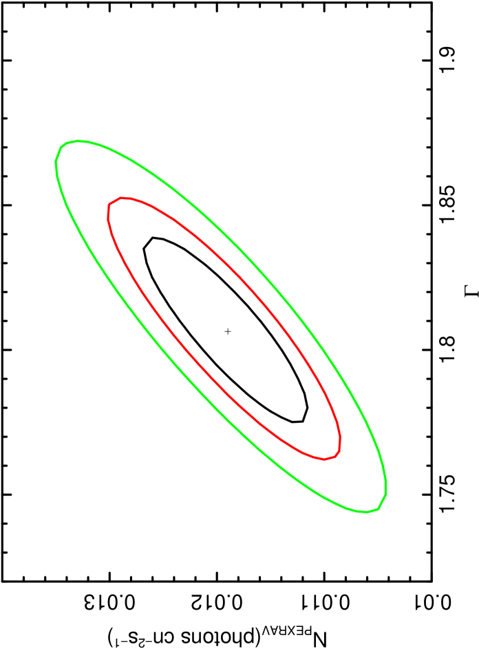
Figure 4: Contour plot showing the 68%, 90%, and 99% confidence levels of the normalisation of the reflected component versus $\Gamma$. Note that the contours have been produced allowing all the other parameters of the best-fit model to vary, including the cross-normalisation between the Suzaku XIS and HXD.

The amount of reflection is consistent with the BeppoSAX measurements of NGC 4507 (Risaliti 2002; Dadina 2007), for which the authors report a reflection fraction ranging from 0.7 to 2.0 (Risaliti 2002), while it is remarkably higher than the value reported from a RXTE measurement ($R=0.4\pm 0.1$, Rivers et al. 2011). The apparent discrepancy between these measurements could be ascribed to the combination of different effects; among them, variability of the primary continuum and of the amount of absorption (see §4). In particular, the Suzaku measurement appears to be, at a first glance, consistent with the scenario proposed for the BeppoSAX observations, where the increase of the reflection fraction was ascribed to a Compton-reflected component remaining constant despite a drop in the primary power-law flux. We note that the RXTE observations were performed in two campaigns one in 1996 and one in 2003, with 94% of the total good exposure time being from the 1996 campaign. During these observations the observed 2–10 keV was a factor of two higher than during the Suzaku one, and thus the lower reflection fraction could be in agreement with this scenario.

However, as already suggested by Rivers et al. (2011), the scenario could be far more complex and also indicative that the reflection component normalisation is responding to a different past illuminating flux. We note however that not only do these works assume different values for the inclination angle, which could affect the measurement of the reflection fraction, but that also the model itself which is adopted for the reflected component is not flawless, indeed it assumes that the reflector is a semi-infinite slab and also its density is assumed to be infinite. More importantly the energy band and spectral resolution of the observations have a strong impact on the measurement of the continuum parameters; for example, the RXTE observations have a lower resolution at the energy of the iron line with respect to the BeppoSAX  and Suzaku  ones, and this has a strong impact on the measurement of the Fe K line/edge properties as well as on the measurement of the amount of reflection and the intrinsic $\Gamma$. The amount of reflection also strongly depends on the model assumed for the X-ray absorber, indeed including the effect of the Compton-down scattering would increase the normalisation of the primary emission and not of the reflected component and thus lower the value of the reflected fraction.

A more detailed description of the variability of this source is presented in §§4 and 4.1, where we compare the historical X-ray spectra obtained for this source, showing that both the amount of absorption and possibly the primary continuum are varying, while the reflected component and the $N_{\mbox{\scriptsize H}}$ of a distant reprocessor remain rather constant. We present a summary of the main parameters of the X-ray emission that can be derived assuming both the standard models and the new model for a toroidal reprocessor, i.e. the mytorus model (Murphy & Yaqoob, 2009).

4 Evidence for a variable absorber

In Fig. 6 we compare the XMM-Newton (red) and the Suzaku XIS & HXD (black) data; a clear difference in the curvature is present between 4 and 8 keV, which is most likely due to a change in the amount of absorption of the primary radiation.

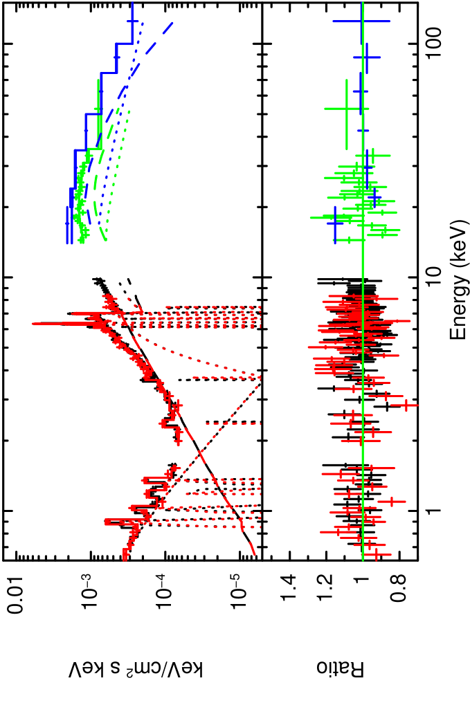
Figure 5: Suzaku  and Swift 0.6–150 keV data and best-fit model (in the electronic version: XIS-FI, black; XIS1, red; HXD-PIN green; Swift-BAT blue) of NGC 4507; data have been rebinned for plotting purposes. The upper panel shows the data and model ($\Gamma\sim 1.8$; N${}_{\mathrm{H}}\sim 8\times 10^{23}$ cm^-2see Table 4 and §3.3), fitted over the 0.6–150 keV band. The lower panel shows the data/model ratio to this model.

To test this hypothesis we applied the Suzaku best-fit model to the XMM-Newton spectrum, allowing the $\mbox{Fe~{}K}\alpha$ emission line parameters as well as all the continuum parameters free to vary (see Table 4). We found a statistically acceptable fit ($\chi^{2}/\mbox{d.o.f.}$ = 633.4/503), which unveiled that the main difference between these two observations can be explained with a lower column density of the intrinsic absorber ($N_{\mbox{\scriptsize H}}^{\mathrm{XMM}}=5.0\pm 0.3\times 10^{23}$ cm^-2and $N_{\mbox{\scriptsize H}}^{\mathrm{SUZAKU}}\sim 8.2\pm 0.6\times 10^{23}$ cm^-2). The normalisation of the primary power-law component also varied between the two observations as well as the amount of reflection; however, we note that there could be some degeneracy between the slope of the primary power-law component and the amount of reflection when lacking a simultaneous high energy observation. We note that without allowing the column density to vary, we could not reproduce the different 2–10 keV spectral curvature observed during the XMM-Newton observation.

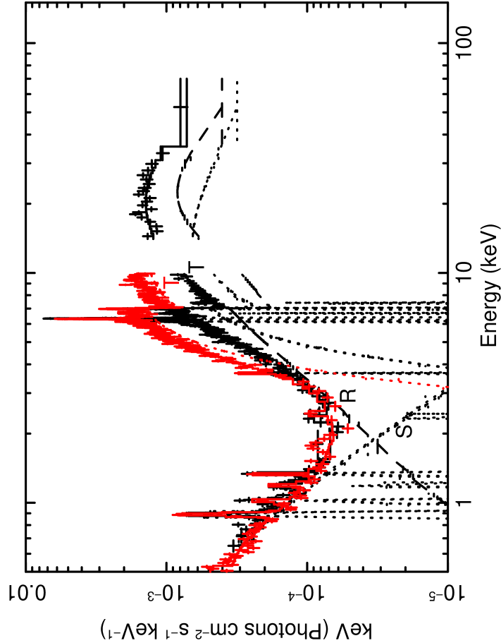
Figure 6: Comparison between the X-ray emission measured with Suzaku in 2007 (black data points in the electronic version) and XMM-Newton  (red data points in the electronic version) in 2001. The continuum model is a standard model; composed of a primary power-law component transmitted trough a neutral absorber (labelled with T), a scattered power-law component (labelled with S) and a Compton reflected component (labelled with R and modelled with pexrav). For the simultaneous fitting we allowed to vary both the $N_{\mbox{\scriptsize H}}$ and the normalisation of the primary power-law component.

To break this degeneracy and better understand the variability of NGC 4507  we reanalysed the 3 BeppoSAX observations of NGC 4507  (hereafter SAX1, SAX2 and SAX3 see Table 1) and, since we are mainly interested in the hard X-ray emission and variability of the spectral curvature, we considered only the MECS and PDS data in the 2–10 keV and 15–200 keV energy range respectively. We adopted the best-fit model of the Suzaku data and we fixed the components responsible for the soft X-ray emission to the Suzaku values. We found that a simple change of the amount of X-ray absorption and the photon index cannot explain the observed variability. We then allowed also the nomalization of the primary continuum and the $\mbox{Fe~{}K}\alpha$  line parameters to vary while constraining the normalization of the reflected component to scale with the primary continuum (i.e. we fixed the ratio $R$, between the primary and reflected component to the one measured during the Suzaku observation). This model represents a situation where the reprocessor responsible for the reflected component responds to the variability of the primary continuum and thus it implies that this absorber should be close to the primary X-ray source. This model did not provide a good fit to SAX1, SAX2 observation ($\chi^{2}/\mbox{d.o.f.}$ =285.9/145, $\chi^{2}/\mbox{d.o.f.}$ = 159.7/108), while it is a statistically acceptable fit for the last BeppoSAX observation ($\chi^{2}/\mbox{d.o.f.}$ =110.9/100), during which NGC 4507 was in a state similar to the Suzaku observation.

Upon allowing also the ratio between the intensity of the reflection component and the primary continuum free to vary (i.e. the parameter $R$) the fits were acceptable and we found $\chi^{2}/\mbox{d.o.f.}$ =159.6/144, $\chi^{2}/\mbox{d.o.f.}$ = 101.5/107 and $\chi^{2}/\mbox{d.o.f.}$ = 108.6/99 for the SAX1, SAX2 and SAX3 observations, respectively. The parameters of these best-fits are reported in Table 4; we note that they are in agreement with the results previously presented in Matt et al. (2004), Risaliti (2002) and Dadina (2007). We found that the Fe K line emission complex is rather constant and also note there is no evidence for variability of the intensity of the reflection component with the BeppoSAX observations.

4.1 A more physical model

This simple test, as described above, shows us that the variability properties of NGC 4507 are more complex than a simple variation of the amount of absorption. We also note that the intrinsic photon index as well as the Fe K emission line complex are not variable, while variations are present in the column density and intensity of the continuum level and thus in the ratio of the reflection component versus the primary continuum. However the absolute flux of the reflection component is consistent with being constant. This in turn tells us that there is a rather stable reprocessor, which is responsible for the Fe K emission lines and the reflected component and which does not appear to respond to the variability of the primary continuum. This could be indicative of distant reprocessor, which does not respond to the variability of the primary continuum. Alternatively as we will discuss later this could indicate a clumpy absorber where the overall distribution of clouds remains rather constant. Given the limitations of the pexrav model, already outlined above (i.e. the geometry and density assumed for the reflector), this simple model does not allow us to derive strong constraints on the true nature of the absorber. Furthermore, by adopting this non physical model the temporal properties of the reprocessor (i.e. the variability of the amount of line-of-sight absorption and Compton reflection) could be highly uncertain and degenerate with respect to the variability of the primary continuum. Finally, the column densities of the X-ray absorber are in the range where the correction for the Compton-down scattering starts to be important. Thus we first included an additional absorber (CABS model in XSPEC) to account for the effect of the Compton-down scattering. We found a similar trend (as the one reported in Table 4) in the normalisations of the primary power-law components and thus in the intrinsic 2–10 keV luminosities, albeit with a larger spread.

Therefore we decided to reanalyse the available spectra using the most recent model for the toroidal reprocessor (Murphy & Yaqoob, 2009), which correctly accounts for the emission expected in transmission (hereafter zeroth order continuum) and reflection and also includes the expected Fe K emission lines ($\mbox{Fe~{}K}\alpha$, Fe K$\beta$ and the Compton shoulder). The calculations at the basis of this new model are all fully relativistic and valid for $N_{\mbox{\scriptsize H}}$ in the Compton-thin and Compton-thick regimes. This new model assumes a uniform and essentially neutral toroidal reprocessor with an opening angle of $60^{\circ}$ with respect to the axis of the system, while we note that the pexrav model assumes a disc/slab geometry for the reflector and thus the parameters derived from this model, such as the covering factor, can not be directly related to a covering factor of the putative torus as well as to the line-of-sight column density. In summary in the mytorus model all the different continuum components (reflected and transmitted components) and the fluorescent emission lines are all treated self-consistently and can thus be all directly related to the key parameters of the matter from which they originate. By adopting this model we were able to determine which component dominates in each energy band (reflected or transmitted components), assess their variability properties and thus better understand the global distribution of the absorber.

4.1.1 A new implementation of the Mytorus model applied to the Suzaku observation

The standard mytorus model, developed for xspec, is composed of three tables of reprocessed spectra calculated assuming that the input spectrum is a power law. These tables correspond to the main model components expected from the interaction of the primary power-law component with a reprocessor that has a toroidal geometry: the distortion to the zeroth-order (transmitted) continuum (MYtorusZ), the reflected continuum (MYtorusS), and the $\mbox{Fe~{}K}\alpha$, Fe K$\beta$ emission-line spectrum (MYtorusL). MYtorusZ is a multiplicative table that contains the pre-calculated transmission factors that distort the incident continuum at all energies due photoelectric absorption.

We first applied this toroidal-reprocessor model (mytorus Murphy & Yaqoob 2009) to the Suzaku observation. The model setup is the following:

phabs$\times$ (apec + apec + A${}_{\rm soft}\times$zpowerlw + 6 GA_em + Fe xxv + Ni K$\alpha$ + MYtorusZ$\times$zpowerlw + A${\rm{}_{R}}\times$ MYtorusS + A$\rm{{}_{L}}\times$ gsmooth $\times$ MYtorusL)

We also included the Fe xxv and Ni K$\alpha$ emission lines as well as a soft power-law component ($A_{\rm soft}\times$zpowerlw) that represents scattering off optically-thin ionised gas (warm or hot), which are not included in the mytorus model. For the soft X-ray emission we kept the 6 Gaussian emission lines (GA_em; see Table 2) and we also included two thermal emission components, which allowed us to tie the photon index of the soft power-law component to the primary one as expected from scattering off optically-thin ionised gas. The normalisations of the mytorus components and of the soft power-law component are all tied together, while the value of the relative normalisations are included in the factors $A_{\rm soft}$, $A{\rm{}_{R}}$ and $A{\rm{}_{L}}$, which are in turn the relative normalisations of the soft power-law component, of the reflected component and of the emission lines. Since we expect the size scale of the scattering/reflecting and line emitting regions to be similar, we initially set $A{\rm{}_{R}}=A{\rm{}_{L}}=1$ to be equal and we set them to 1. We note that we can not interpret any difference between these two factors as a difference in the size scales of these zones since these constants also include the effects of the transfer functions of the reflected continuum and line spectrum. The gsmooth component is the broadening of the Fe K emission lines and it is actually composed of two Gaussian convolution components, one is the actual broadening of the $\mbox{Fe~{}K}\alpha$ emission line while the second component accounts for the weak residual instrumental broadening as measured with the calibration sources ($\sigma<15$ eV, with a $\sqrt{E}$ dependence).

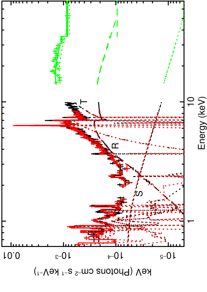
Figure 7: The 0.5–70 keV Suzaku  spectra when fitted with the mytorus model (in the electronic version: XIS-FI, black; XIS1, red; HXD-PIN green). The dashed lines represent the reflected component (marked with R), the dotted lines are the transmitted component (marked with T) and the scattered component (marked with S) from ionised gas.

An inspection of the Suzaku spectra shows that above 8 keV we are dominated by the primary component, transmitted through the reprocessor, which is mainly constrained by the high-energy excess above 10 keV, while the reflected component dominates below 8 keV, where the strong emission lines from the Fe K$\alpha$, Ca K$\alpha$ and S xiv K$\alpha$ are present (see Fig.  7). This is analogous to what is observed adopting the old pexrav model (see Fig. 5, upper panel) and it is also in agreement with the variability of the normalisation of the primary power-law component as suggested in section §4.

We note that in the standard configuration of the mytorus model, we cannot account self-consistently for the requirement of a strong transmitted component emerging at higher energies, the intense Fe K emission lines and a dominant reflected component below 8 keV. In particular, if we adopt the standard toroidal geometry with the inclination angles (between the axis of the torus and the observer’s line of sight) of the two components tied together and if we do not allow the normalisations of the reflected component to vary with respect to the normalisation of the zeroth order continuum strong residuals are present below 10 keV. Keeping $A{\rm{}_{R}}$ and $A{\rm{}_{L}}$ tied to each other, we found that a cross-normalization factor of $A{\rm{}_{R}}\sim 3$ is indeed required to reproduce the shape of the 4–10 keV continuum and the intensity of the Fe K emission lines, where the reflected component dominates. This forces the inclination angle between the axis of the torus and the observer’s line of sight to a grazing value ($\sim 60^{\circ}$).

Although we cannot rule out this scenario, we must allow for the possibility of a different geometry taking into account all the information that we obtained from the historical X-ray observations of NGC 4507  which suggested that: a) the column density of the line of sight (los) absorber varies; b) the flux of the $\mbox{Fe~{}K}\alpha$ remains rather stable, suggesting the presence of a constant and distant reprocessor and c) the primary continuum is also variable. Physically, the situation we want to model corresponds to a patchy reprocessor in which the reflected continuum is observed from reflection in matter on the far-side of the X-ray source, without intercepting any other “clouds,” and the zeroth-order continuum corresponds to extinction by clouds in the line-of-sight. In practice this corresponds to allowing the column densities of the zeroth-order and reflected continua to be independent of each other; we thus followed the methodology discussed by Yaqoob 2012 applied to the modelling of the broadband X-ray emission of NGC 4945. By decoupling these two components, we can also allow the reflected and transmitted components to have a different temporal behaviour. We can do this by decoupling the inclination angle parameters for the line-of-sight (zeroth-order) continuum passing through the reprocessor and for the reflected continuum from the reprocessor and allowing the column densities responsible for the reprocessing of the primary emission to be independent. The reflected continuum (and the fluorescent line emission, which is tied to it) is not extinguished by another column.

The inclination angle of the zeroth-order component is now irrelevant (so it is fixed at 90 degrees), and the inclination angle for the reflected continuum is fixed at 0 degrees because the effect of the inclination angle on the shape of the reflected continuum is not sufficiently large (in terms of spectral fitting) if the reflected continuum is observed in reflection only. Furthermore, since we are trying to model a patchy reprocessor as suggested from the column density variations, the inclination angle may not be meaningful. We note also that we cannot interpret the ratio between the normalisations of the reflected and transmitted components simply as a covering factor of the reprocessors. Although the constant in front of the reflected continuum ($A_{\rm R}$) does contain some information on the covering factor, that information cannot be decoupled from the effect of time delays between variability of the direct X-ray continuum and the reprocessed X-ray continuum. This is because the light-crossing time of the reprocessor is likely to be much longer than the direct X-ray continuum variability timescale, so the magnitude of the reflected continuum corresponds to the reprocessed direct continuum that is averaged over a timescale that is longer than the reprocessor light-crossing time. This decoupling of the mytorus model is close to the standard procedure used while fitting with PEXRAV plus an absorbed power-law component. However there are several differences, in particular the column density of the reflector is also a free parameter and the Fe emission line intensities are calculated self consistently.

The model then yields a $\chi^{2}/\mbox{d.o.f.}$ = 392.5/359 and a mean line-of-sight column density of $N_{\mbox{\scriptsize H}}=9.4$${}^{+0.2}_{-0.2}$$\times 10^{23}$ cm^-2, while the angle-averaged column density of the reflector (out of the line-of-sight) is $N_{\mbox{\scriptsize H}}=2.6$${}^{+0.2}_{-0.2}$$\times 10^{23}$ cm^-2, where also the Fe K emission lines are produced. The photon index is found to be $\Gamma=1.68$${}^{+0.03}_{-0.03}$ and the normalisation of the primary continuum is $1.91^{+0.16}_{-0.25}\times 10^{-2}$ ph cm^-2 s^-1. We also allowed the constant for the normalisation of the reflected continuum ($A_{\rm R}$) to vary and we found that it is consistent with 1 ($A_{\rm R}=1.1\pm 0.2$). Finally, we note that now the measured velocity broadening of the $\mbox{Fe~{}K}\alpha$  emission line is $\sigma_{v}<29$ eV.

Table 3: Summary of the X-ray emission lines detected in the 6–8 keV energy range. The energies of the lines are quoted in the rest frame. Fluxes and identifications are reported in column 2 and 3. The EW are reported in column 4 and they are calculated against the total observed continuum at their respective energies. In column 5 the improvement of fit is shown with respect to the continuum model, the value for the model with no lines is $\chi^{2}/\mbox{d.o.f.}$ =1918.9/375.

Energy	Flux	ID	EW	$\Delta\chi^{2}$
(keV)	($10^{-6}$ph cm-2 s-1)		(eV)
(1)	(2)	(3)	(4)	(5)
6.408${}^{+0.005}_{-0.004}$	52.4${}^{+3.7}_{-5.1}$	$\mbox{Fe~{}K}\alpha$	490${}^{+40}_{-50}$	1427.4
7.07${}^{+0.02}_{-0.02}$	10.0${}^{+1.8}_{-1.8}$	Fe K$\beta$	81${}^{+23}_{-13}$	82.0
6.73 ${}^{+0.05}_{-0.06}$	3.1${}^{+1.6}_{-1.6}$	Fe xxv	27 ${}^{+15}_{-13}$	8.1
7.50${}^{+0.07}_{-0.08}$	2.3${}^{+1.5}_{-1.4}$	Ni K$\alpha$	37${}^{+24}_{-23}$	6.7

Table 4: Comparison between the best fit values for the continuum and $\mbox{Fe~{}K}\alpha$ emission line for the Suzaku  XMM-Newton and BeppoSAX  observations. The fluxes are corrected only for Galactic absorption.

Parameter	Suzaku	XMM-Newton	SAX1	SAX2	SAX3
DATE	2007-12	2001-01	1997-07	1998-07	1999-01
$N_{\rm H}$ ($10^{23}$ cm-2)	$8.2_{-0.6}^{+0.6}$	$5.0^{+0.2}_{-0.3}$	7.0${}^{+0.4}_{-0.5}$	6.2${}^{+0.7}_{-0.3}$	7.2${}^{+2.9}_{-1.6}$
$\Gamma_{\mathrm{Hard}}$	$1.81_{-0.04}^{+0.04}$	$1.76_{-0.04}^{+0.05}$	1.77${}^{+0.03}_{-0.05}$	1.72${}^{+0.07}_{-0.1}$	1.6${}^{+0.1}_{-0.1}$
Normalisation ($10^{-2}$ ph cm-2 s${-1}$)	$0.64_{-0.11}^{+0.13}$	$1.25_{-0.06}^{+0.06}$	2.52${}^{+0.22}_{-0.33}$	1.70${}^{+0.19}_{-0.23}$	0.62${}^{+0.48}_{-0.23}$
$\Gamma_{\mathrm{Soft}}$	3.8${}^{+0.2}_{-0.2}$	3.7${}^{+0.1}_{-0.1}$	..	..	..
Normalisation ($10^{-4}$ ph cm-2 s-1)	$1.70_{-0.09}^{+0.09}$	$1.37_{-0.05}^{+0.06}$	..	..	..
$A_{\mathrm{pexrav}}$ ($10^{-2}$ph cm-2 s-1)	$1.19^{+0.09}_{-0.09}$	$0.88^{+0.14}_{-0.13}$	1.6${}^{+0.2}_{-0.3}$	1.2${}^{+0.3}_{-0.3}$	1.0${}^{+0.5}_{-0.4}$
Fe K$\alpha$ (keV)	$6.408_{-0.004}^{+0.005}$	$6.39_{-0.02}^{+0.04}$	6.39${}^{+0.10}_{-0.09}$	6.58${}^{+0.11}_{-0.12}$	6.42${}^{+0.07}_{-0.07}$
$I_{\mathrm{FE}}$ ($10^{-5}$ph cm-2 s-1)	$5.24^{+0.51}_{-0.37}$	$4.36^{+0.43}_{-0.41}$	4.7${}^{+1.7}_{-1.8}$	6.7${}^{+2.0}_{-2.2}$	5.9${}^{+1.5}_{-1.5}$
$EW_{\mathrm{FE}}$ (eV)	490${}^{+40}_{-50}$	190${}^{+20}_{-100}$	140${}^{+80}_{-60}$	225${}^{+65}_{-90}$	400${}^{+90}_{-120}$
F ${}_{(0.5-2\;\mathrm{keV})}$ ($10^{-13}$ erg cm-2 s-1)	$\sim 4.8$	$\sim 4.9$	…	…	…
F${}_{(2-10\;\mathrm{keV})}$ ($10^{-11}$ erg cm-2 s-1)	$\sim 0.6$	$\sim 1.2$	$\sim 1.8$	$\sim 1.6$	$\sim 0.8$
L${}_{(2-10\;\mathrm{keV})}$ ($10^{43}$ erg s-1)	$\sim 0.9$	$\sim 1.5$	$\sim 2.8$	$\sim 2.2$	$\sim 1.0$

Table 5: Comparison between the best fit values for the continuum and $N_{\mbox{\scriptsize H}}$ for the Suzaku, XMM-Newton  and BeppoSAX observations when fitted with the mytorus model. The fluxes are corrected only for Galactic absorption, while the luminosities are corrected also for the intrinsic absorption, which includes the effect of the Compton-down scattering.

Parameter	Suzaku	XMM-Newton	SAX1	SAX2	SAX3
	2007-12	2001-01	1997-07	1998-07	1999-01
$\Gamma$	$1.68_{-0.03}^{+0.03}$	$1.68^{f}$	1.62${}^{+0.03}_{-0.03}$	1.66${}^{+0.04}_{-0.05}$	1.63${}^{+0.08}_{-0.07}$
Normalisation ($10^{-2}$ ph cm-2 s${-1}$)	$1.91_{-0.25}^{+0.16}$	$1.56_{-0.12}^{+0.05}$	2.89${}^{+0.32}_{-0.35}$	2.98${}^{+0.49}_{-0.52}$	2.12${}^{+0.87}_{-0.61}$
$N_{\rm H\;transmitted}$ ($10^{23}$ cm-2)	$9.38_{-0.24}^{+0.25}$	$4.66^{+0.10}_{-0.27}$	6.33${}^{+0.29}_{-0.35}$	6.46${}^{+0.45}_{-0.46}$	8.58${}^{+0.10}_{-0.96}$
$N_{\rm H\;reflected}$ ($10^{23}$ cm-2)	$2.56_{-0.17}^{+0.20}$	$3.54^{+1.26}_{-0.41}$	2.64${}^{+0.88}_{-0.50}$	2.40${}^{+0.85}_{-0.89}$	2.37${}^{+1.29}_{-1.05}$
F${}_{(2-10\;\mathrm{keV})}$ ($10^{-11}$ erg cm-2 s-1)	$\sim 0.6$	$\sim 1.2$	$\sim 1.7$	$\sim 1.6$	$\sim 0.9$
L${}_{(2-10\;\mathrm{keV})}$ ($10^{43}$ erg s-1)	$\sim 2.5$	$\sim 2.1$	$\sim 4.0$	$\sim 4.1$	$\sim 3.0$

4.1.2 Mytorus model for Suzaku, XMM-Newton and BeppoSAX

We then applied the same model to the XMM-Newton observation. For simplicity, since there is no evidence of variability of the soft X-ray emission and taking into account that the Gaussian emission lines plus the thermal components are simple phenomenological models, we decided to keep fixed the main parameters of the latter to the Suzaku best-fit model. Furthermore, since we lack of simultaneous observation above 10 keV we also fixed the photon index to the one measured with Suzaku and for simplicity at first we kept the constant of the relative emission line component ($A_{\mathrm{L}}$) fixed to 1. We found that the out of los column density was comparable to the one measured during the Suzaku observation ($N_{\mbox{\scriptsize H}}=3.5$ ${}^{+1.3}_{-0.4}$$\times 10^{23}$ cm^-2) while the los absorbing column density was $N_{\rm{H}}=4.7^{+0.1}_{-0.3}\times 10^{23}$ cm^-2($\chi^{2}/$dof=$600.5/498$).

In contrast with the previous modelling with pexrav, we can now attempt to investigate also the relative intensity of the zeroth-order and reflected components. We found that the intensity of the zeroth order changed from $(1.91^{+0.16}_{-0.25})\times 10^{-2}$ ph cm^-2 s^-1 to $(1.56^{+0.05}_{-0.12})\times 10^{-2}$ ph cm^-2 s^-1 during the XMM-Newton  and Suzaku pointing respectively.This suggests that no strong variation of the primary continuum is required to explain the observed 2–10 keV spectral differences, but the main driver of the variations is the change in the column density of the line-of-sight absorber.

Finally, we applied the same model to the 3 BeppoSAX observations, allowing also the photon index to vary, and we found that the column density of the out of the los absorber remained stable and it was comparable (within the errors) to the one measured with Suzaku and XMM-Newton, ($N_{\mbox{\scriptsize H}}=2.6$ ${}^{+0.9}_{-0.5}$$\times 10^{23}$ cm^-2, $N_{\mbox{\scriptsize H}}=2.4$ ${}^{+0.9}_{-0.9}$$\times 10^{23}$ cm^-2 and $N_{\mbox{\scriptsize H}}=2.4$ ${}^{+1.3}_{-0.1}$$\times 10^{23}$ cm^-2 for SAX1, SAX2 and SAX3 respectively). The column density of the los absorber varied with a similar trend as the one measured with the pexrav-based model ($N_{\mbox{\scriptsize H}}=6.3$ ${}^{+0.3}_{-0.4}$$\times 10^{23}$ cm^-2, $N_{\mbox{\scriptsize H}}=6.5$ ${}^{+0.5}_{-0.5}$$\times 10^{23}$ cm^-2and $N_{\mbox{\scriptsize H}}=8.6$ ${}^{+0.1}_{-1.0}$$\times 10^{23}$ cm^-2for SAX1, SAX2 and SAX3 respectively), the intensity of the primary continuum components also varied. In particular, the intensity of the primary continuum was higher in the SAX1 and SAX2 observation and in SAX3. However, due to the lower statistics of the BeppoSAX data these measurements have a large error which prevent us from deriving a clear picture. We note that there is no evidence for a variation of the photon index.

5 Discussion and conclusions

Detailed X-ray spectral analysis of the Suzaku data confirms the complexity of the X-ray emission from NGC 4507. Thanks to the wide-band spectrum covering from 0.6 keV to 70 keV, we have now obtained the most reliable deconvolution of all the spectral components. The X-ray continuum is composed of three components: a heavily absorbed power-law component, a reflected component and a weak soft scattered component. We analysed the Suzaku and the historical observations of NGC 4507 adopting both a standard model as well as a new toroidal reprocessor model. With either of these two approaches we found that during the Suzaku observation the 2–10 keV emission of NGC 4507 was dominated by the reflected emission, while above 10 keV the spectrum was dominated by the highly absorbed transmitted component.

The soft X-ray emission can be well described with a superposition of a power-law component, which is considered to be the scattered light from ionised, optically-thin gas, and several emission lines. These emission lines were already detected with the ASCA observation (Comastri et al. 1998). As already shown with the XMM-Newton observation (Matt et al., 2004), the wide range of ionisation implied by these lines is indicative of the presence of at least two photo- or collisionally- ionised emitters. This is confirmed by a recent deep XMM-Newton observation obtained by our group within a monitoring program of NGC 4507. The analysis of the single observations showed also that as seen in other Seyfert 2s the soft X-ray emission did not vary, implying that the emitters responsible for this emission are located outside the variable X-ray absorber (Marinucci et al. 2012b, Wang et al private communication).

5.1 The X-ray absorber

In the last two decades NGC 4507, which is one of the X-ray brightest and nearby Seyfert 2 galaxies, has been observed several times with all the different X-ray observatories; NGC 4507 displayed an observed 2–10 keV flux ranging from $0.6-1.3\times 10^{-11}$erg cm^-2 s^-1; furthermore these X-ray observations showed long-term $N_{\mathrm{H}}$ variability, which changes by a factor of 2, and also possible variability of the intrinsic continuum (Risaliti 2002). The Suzaku observation caught the source with a low observed 2–10 keV flux, similar to the last BeppoSAX observation (SAX3), which was also characterised by the highest measured column density of the X-ray absorber ($8-9\times 10^{23}$ cm^-2). Our analysis of the XMM-Newton  BeppoSAX, and Suzaku observations shows that, independently from the assumed model (i.e. mytorus or the standard pexrav one) the X-ray absorber in NGC 4507 varies from $\sim 5\times 10^{23}$ cm^-2 to $\sim 9\times 10^{23}$ cm^-2  on $\sim 6$ months time scale between the observations.

Assuming a spherical geometry for the obscuring clouds, and that they are moving with Keplerian velocities (as in the case of NGC 1365; Risaliti et al. 2007), then there is a first order simple relation between the crossing time of such obscuring cloud, the linear dimension and distance of the obscuring cloud and the size of the X-ray source (see Marinucci et al. 2012b). From this work, since no variability is found on a short time scales, during the long Suzaku observation, we can infer that the variability occurs on a time scale between 2 days (as the elapsed time of the Suzaku observation was $\sim 180$ ks) and six months (as the elapsed time between the second and the third BeppoSAX observations). Following the same argument proposed for NGC 1365 (Risaliti et al. 2007), where similar assumptions are used, then a possible scenario could be that the variable absorber is located a distance greater than 0.01 pc from the X-ray source (i.e. not closer than the Broad Line Region). Thus a possible scenario, where the classical uniform absorber still exists is that there are multiple absorbers. One is the classical and uniform pc-scale absorber (i.e. the torus), which is responsible for the Fe K emission line and the constant reflected component; while the $N_{\mathrm{H}}$ variability requires the presence of a second and clumpy absorber that could be coincident with the outer BLRs. We note that the observations presented here do not span the possible time-scale expected for a variable absorber located between the BLR and the pc-scale absorber.

However a simpler scenario could be that the variability is due to a certain degree of clumpiness of a single absorber itself, as for the clumpy torus model (Nenkova et al. 2002, 2008; Elitzur & Shlosman 2006). In this scenario, if the distribution of clouds remains rather constant, we can have a constant reflected component while at the same time changes of the line-of-sight $N_{\mbox{\scriptsize H}}$. Recently our group obtained an XMM-Newton monitoring campaign of NGC 4507  consisting of six observations performed every 10 days, this monitoring confirmed that the $N_{\mbox{\scriptsize H}}$ variability occurs on relatively long time scale (between 1.5 and 4 months), supporting the scenario of a clumpy pc-scale absorber (Marinucci et al. 2012b). A long term variability or lack of certain components cannot be simply used to infer the location of the reprocessor itself in terms of time delays between the reflected component and the primary continuum. As discussed in several works on the spectral variability of well monitored Seyfert 1s (e.g MCG-6-30-15 Miller et al. 2008; Mrk 766 Miller et al. 2007), the apparent variability of the observed continuum level could be due to changes of the los covering fraction and not of the intrinsic continuum level. Thus the reflected emission would remain rather constant even for closer in and variable absorbers.

Stronger evidence for the presence of a pc-scale reflector can be derived from the analysis of the $\mbox{Fe~{}K}\alpha$ emission line profile. We note that $\mbox{Fe~{}K}\alpha$ emission line is rather constant and narrow with no evidence of an additional strong broad component; its width, measured with Suzaku, is $\sigma<30$ eV (or $\sigma_{v}<1400$ km s^-1) and consistent with the Chandra upper limits, $\sigma_{v}<1200$ km s^-1 ($FWHM<3000$ km s^-1). The measured $FWHM$ of the H$\alpha$ ($\sim 5000$ km s^-1; Moran et al. 2000) is marginally higher than the Chandra upper limit on the $\mbox{Fe~{}K}\alpha$  $FWHM$. This suggests that the $\mbox{Fe~{}K}\alpha$  is produced either in the outer part of the BLRs or in a pc-scale absorber; in agreement with a scenario where there is a distant and stable reprocessor, which could be identified with the classical torus. A similar result has been presented by Shu et al. (2011), where the authors compared the FWHM of the $\mbox{Fe~{}K}\alpha$ emission line (measured with the Chandra HETG) of a sample of Seyfert 2s (including NGC 4507) with the $FWHM$ of the optical lines. They suggested that the $\mbox{Fe~{}K}\alpha$ emitter is a factor 0.7–11 times larger than the optical line-emitting region and located at a distance of about $r\sim 3\times 10^{4}r_{g}$ (where $r_{g}$ is the gravitational radius defined as $r_{g}=GM/c^{2}$). In particular from the estimated black hole mass for NGC 4507  of M${}_{\mathrm{BH}}\sim 4\times 10^{7}$ M_⊙ (Bian & Gu 2007) and assuming Keplerian motion, the upper limit on its $FWHM$ implies that the Fe K$\alpha$ emission line is produced at a distance $r>0.02$ pc from the central BH. We note that assuming the larger BH mass (M${}_{\mathrm{BH}}\sim 2.5\times 10^{8}$ M_⊙) reported by Winter et al. (2009) would place the absorber at a distance $R>0.06$ pc and the location of the $\mbox{Fe~{}K}\alpha$  at $r>0.1$ pc.

In terms of the global picture for the location and structure of the X-ray absorbers, we have now several examples of obscured AGNs with short-term variation unveiling that a significant fraction of the absorbing clouds are located within the BLR. However there is also evidence for the presence of a pc-scale absorber as predicted in the Unified Model of AGNs. This absorber is confirmed by the ubiquitous presence of the narrow $\mbox{Fe~{}K}\alpha$ emission line and the Compton reflection component, which do not show strong variability between observations even in case of a variable intrinsic continuum and/or variable neutral absorber (e.g. NGC 7582 Piconcelli et al. 2007; Bianchi et al. 2009, NGC 4945; Marinucci et al. 2012a; Yaqoob 2012; Itoh et al. 2008). Another piece of evidence for the presence of a distant reprocessor comes from the comparison between the Chandra, XMM-Newton  and Suzaku observations of the bright Seyfert 2 NGC 4945 (Marinucci et al. 2012a; Yaqoob 2012), where a detailed spectral, variability and imaging analysis unveiled that the emitting region responsible for the $\mbox{Fe~{}K}\alpha$  line and the Compton-scattered continuum has a low covering factor and it is most likely located at a distance $>30-50$ pc. In this framework the relatively long-term absorption variability shown by NGC 4507 confirms that the location and structure of the X-ray absorber is complex and that absorption in type 2 AGNs could occur on different scales and that there may not be a universal single and uniform absorber.

Finally, by adopting the standard pexrav model, even with the broad band X-ray observations available for NGC 4507, we cannot assess the role of the possible variability of the primary continuum or estimate the column density of the reprocessor responsible for the Fe K$\alpha$ emission line. Interestingly, the fit with the decoupled mytorus model, which can mimic either a patchy toroidal reprocessor or a situation where there are two reprocessors (one seen in ”transmission”, dominating the high-energy spectrum, and one seen in reflection), allows us to measure these column densities and the possible variability of the primary continuum. Although the decoupled mytorus model closely resembles the classical combination of pexrav (slab reflection component) and an absorbed power-law component, the column densities of both the reprocessors (“reflector” and “absorber”) are treated independently and self-consistently with the emission of the Fe K line. Table 5 shows that the line-of-sight obscuration of the reprocessor seen in transmission varies by $\Delta N_{\mathrm{H}}\sim 5\times 10^{23}$ cm^-2, while there is a constant reprocessor with a column density of $\sim 2-3\times 10^{23}$cm^-2, which is the one responsible for the Fe K$\alpha$ emission line. The intrinsic X-ray luminosity ranges from $L_{(2-10\;\mathrm{keV})}\sim 2.1\times 10^{43}$ erg s^-1to $L_{(2-10\;\mathrm{keV})}\sim 4.1\times 10^{43}$ erg s^-1. While we observe intrinsic variation of primary power-law intensity, the $N_{\mbox{\scriptsize H}}$ variablity drives the spectral changes between 2-10 keV. Conversely, the reflection and emission line components are not observed to vary.

We note that the behaviour of the line-of-sight column and reflection fraction with respect to the intrinsic continuum going from the BeppoSAX to the Suzaku observation strongly depends on the adopted model for the reprocessor. Indeed as can be seen comparing Table 4 and  5, by adopting the combination of pexrav and an absorbed power-law component, we would infer that NGC 4507  was intrinsically brighter and less obscured during the XMM-Newton observation. However, no such trend is inferred with the mytorus model, where the opposite is the case (i.e. the more absorbed Suzaku observation has the higher primary power-law normalisation). Only future monitoring campaigns with broad band observatories such as ASTRO-H (i.e. with instrument with an high effective area above 10 keV as well as high spectral resolution at the $\mbox{Fe~{}K}\alpha$ line) will allow monitoring of sources like NGC 4507. These observations will allow to investigate the variability of the harder continuum simultaneously providing a detailed investigation of the profile of the $\mbox{Fe~{}K}\alpha$ emission line, thus establishing the geometry and location of the “stable” and variable reprocessors.

References

- Antonucci (1993) Antonucci, R. 1993, ARA&A, 31, 473
- Arnaud (1996) Arnaud, K. A. 1996, Astronomical Data Analysis Software and Systems V, 101, 17
- Awaki et al. (1991) Awaki, H., Kunieda, H., Tawara, Y., & Koyama, K. 1991, PASJ, 43, L37
- Bassani et al. (1995) Bassani, L., Malaguti, G., Jourdain, E., Roques, J. P., & Johnson, W. N. 1995, ApJ, 444, L73
- Bassani et al. (2006) Bassani, L., Molina, M., Malizia, A., et al. 2006, ApJ, 636, L65
- Beckmann et al. (2009) Beckmann, V., Soldi, S., Ricci, C., et al. 2009, A&A, 505, 417
- Behar et al. (2010) Behar, E., Kaspi, S., Reeves, J., et al. 2010, ApJ, 712, 26
- Bian & Gu (2007) Bian, W., & Gu, Q. 2007, ApJ, 657, 159
- Bianchi et al. (2006) Bianchi, S., Guainazzi, M., & Chiaberge, M. 2006, A&A, 448, 499
- Bianchi et al. (2009) Bianchi, S., Piconcelli, E., Chiaberge, M., et al. 2009, ApJ, 695, 781
- Bianchi et al. (2012) Bianchi, S., Maiolino, R., & Risaliti, G. 2012, Advances in Astronomy, 2012,
- Boldt (1987) Boldt, E. 1987, Phys. Rep., 146, 215
- Comastri et al. (1998) Comastri, A., Vignali, C., Cappi, M., Matt, G., Audano, R., Awaki, H., & Ueno, S. 1998, MNRAS, 295, 443
- Dadina (2007) Dadina, M. 2007, A&A, 461, 1209
- Dickey & Lockman (1990) Dickey, J. M., & Lockman, F. J. 1990, ARA&A, 28, 215
- Elvis (2000) Elvis, M. 2000, ApJ, 545, 63
- Elvis et al. (2004) Elvis, M., Risaliti, G., Nicastro, F., Miller, J. M., Fiore, F., & Puccetti, S. 2004, ApJ, 615, L25
- Elitzur & Shlosman (2006) Elitzur, M., & Shlosman, I. 2006, ApJ, 648, L101
- Elitzur (2012) Elitzur, M. 2012, ApJ, 747, L33
- Fukazawa et al. (2011) Fukazawa, Y., Hiragi, K., Mizuno, M., et al. 2011, ApJ, 727, 19
- Gruber et al. (1999) Gruber, D. E., Matteson, J. L., Peterson, L. E., & Jung, G. V. 1999, ApJ, 520, 124
- Guainazzi & Bianchi (2007) Guainazzi, M., & Bianchi, S. 2007, MNRAS, 374, 1290
- Horst et al. (2006) Horst, H., Smette, A., Gandhi, P., & Duschl, W. J. 2006, A&A, 457, L17
- Itoh et al. (2008) Itoh, T., Done, C., Makishima, K., et al. 2008, PASJ, 60, 251
- Jaffe et al. (2004) Jaffe, W., Meisenheimer, K., Röttgering, H. J. A., et al. 2004, Nature, 429, 47
- Kallman et al. (2004) Kallman, T. R., Palmeri, P., Bautista, M. A., Mendoza, C., & Krolik, J. H. 2004, ApJS, 155, 675
- Kokubun et al. (2007) Kokubun, M., et al. 2007, PASJ, 59, 53
- Koyama et al. (2007) Koyama, K., et al. 2007, PASJ, 59, 23
- Kriss et al. (1980) Kriss, G. A., Canizares, C. R., & Ricker, G. R. 1980, ApJ, 242, 492
- Lutz et al. (2004) Lutz, D., Maiolino, R., Spoon, H. W. W., & Moorwood, A. F. M. 2004, A&A, 418, 465
- Magdziarz & Zdziarski (1995) Magdziarz, P., & Zdziarski, A. A. 1995, MNRAS, 273, 837
- Maiolino et al. (2010) Maiolino, R., Risaliti, G., Salvati, M., et al. 2010, A&A, 517, A47
- Malizia et al. (2009) Malizia, A., Stephen, J. B., Bassani, L., et al. 2009, MNRAS, 399, 944
- Marinucci et al. (2012a) Marinucci, A., Risaliti, G., Wang, J., et al. 2012a, MNRAS, 423, L6
- Marinucci et al. (2012b) Marinucci, A. et al. MNRAS submitted
- Matt (2002) Matt, G. 2002, MNRAS, 337, 147
- Matt et al. (2004) Matt, G., Bianchi, S., D’Ammando, F., & Martocchia, A. 2004, A&A, 421, 473
- Mewe et al. (1985) Mewe, R., Gronenschild, E. H. B. M., & van den Oord, G. H. J. 1985, A&AS, 62, 197
- Miller et al. (2007) Miller, L., Turner, T. J., Reeves, J. N., et al. 2007, A&A, 463, 131
- Miller et al. (2008) Miller, L., Turner, T. J., & Reeves, J. N. 2008, A&A, 483, 437
- Miller et al. (2010) Miller, L., Turner, T. J., Reeves, J. N., Lobban, A., Kraemer, S. B., & Crenshaw, D. M. 2010, MNRAS, 403, 196
- Mitsuda et al. (2007) Mitsuda, K., et al. 2007, PASJ, 59, 1
- Moran et al. (2000) Moran, E. C., Barth, A. J., Kay, L. E., & Filippenko, A. V. 2000, ApJ, 540, L73
- Murphy & Yaqoob (2009) Murphy, K. D., & Yaqoob, T. 2009, MNRAS, 397, 1549
- Nenkova et al. (2002) Nenkova, M., Ivezić, Ž., & Elitzur, M. 2002, ApJ, 570, L9
- Nenkova et al. (2008) Nenkova, M., Sirocky, M. M., Nikutta, R., Ivezić, Ž., & Elitzur, M. 2008, ApJ, 685, 160
- Palmeri et al. (2003) Palmeri, P., Mendoza, C., Kallman, T. R., Bautista, M. A., & Meléndez, M. 2003, A&A, 410, 359
- Piconcelli et al. (2007) Piconcelli, E., Bianchi, S., Guainazzi, M., Fiore, F., & Chiaberge, M. 2007, A&A, 466, 855
- Poncelet et al. (2006) Poncelet, A., Perrin, G., & Sol, H. 2006, A&A, 450, 483
- Poutanen & Svensson (1996) Poutanen, J., & Svensson, R. 1996, ApJ, 470, 249
- Puccetti et al. (2007) Puccetti, S., Fiore, F., Risaliti, G., et al. 2007, MNRAS, 377, 607
- Reeves et al. (2009) Reeves, J. N., O’Brien, P. T., Braito, V., et al. 2009, ApJ, 701, 493
- Risaliti (2002) Risaliti, G. 2002, A&A, 386, 379
- Risaliti et al. (2002) Risaliti, G., Elvis, M., & Nicastro, F. 2002, ApJ, 571, 234
- Risaliti et al. (2005) Risaliti, G., Bianchi, S., Matt, G., Baldi, A., Elvis, M., Fabbiano,G., & Zezas, A. 2005, ApJ, 630, L129
- Risaliti et al. (2007) Risaliti, G., Elvis, M., Fabbiano, G., et al. 2007, ApJ, 659, L111
- Risaliti et al. (2009) Risaliti, G., et al. 2009, MNRAS, 393, L1
- Risaliti et al. (2010) Risaliti, G., Elvis, M., Bianchi, S., & Matt, G. 2010, MNRAS, 406, L20
- Risaliti et al. (2011) Risaliti, G., Nardini, E., Salvati, M., et al. 2011, MNRAS, 410, 1027
- Rivers et al. (2011) Rivers, E., Markowitz, A., & Rothschild, R. 2011, ApJS, 193, 3
- Shu et al. (2011) Shu, X. W., Yaqoob, T., & Wang, J. X. 2011, ApJ, 738, 147
- Spergel et al. (2003) Spergel, D. N., et al. 2003, ApJS, 148, 175
- Takahashi et al. (2007) Takahashi, T., et al. 2007, PASJ, 59, 35
- Tatum et al. (2012) Tatum, M., Turner, T.J., Miller, L., Reeves, J.N., 2012, ApJ, submitted
- Tueller et al. (2010) Tueller, J., et al. 2010, ApJS, 186, 378
- Turner et al. (1997) Turner, T. J., George, I. M., Nandra, K., & Mushotzky, R. F. 1997, ApJ, 488, 164
- Turner et al. (2000) Turner, T. J., Perola, G. C., Fiore, F., et al. 2000, ApJ, 531, 245
- Turner et al. (2007) Turner, T. J., Miller, L., Reeves, J. N., & Kraemer, S. B. 2007, A&A, 475, 121
- Turner et al. (2008) Turner, T. J., Reeves, J. N., Kraemer, S. B., & Miller, L. 2008, A&A, 483, 161
- Turner & Miller (2009) Turner, T. J., & Miller, L. 2009, A&A Rev., 17, 47
- Turner et al. (2009) Turner, T. J., Miller, L., Kraemer, S. B., Reeves, J. N., & Pounds, K. A. 2009, ApJ, 698, 99
- Turner et al. (2012) Turner, T. J., Miller, L., & Tatum, M. 2012, American Institute of Physics Conference Series, 1427, 165
- Urry & Padovani (1995) Urry, C. M., & Padovani, P. 1995, PASP, 107, 803
- Winter et al. (2009) Winter, L. M., Mushotzky, R. F., Reynolds, C. S., & Tueller, J. 2009, ApJ, 690, 1322
- Yaqoob & Murphy (2011) Yaqoob, T., & Murphy, K. D. 2011, MNRAS, 412, 277
- Yaqoob (2012) Yaqoob, T. 2012, MNRAS, 423, 3360