Node-less atomic wave functions, Pauli repulsion and systematic projector augmentation

Abstract

A construction of node-less atomic orbitals and energy-dependent, node-reduced partial waves is presented, that contains the full information of the atomic eigenstates and that allows to represent the scattering properties in a transparent manner. By inverting the defining Schrödinger equation, the Pauli repulsion by the core electrons can be represented as effective potential. This construction also provides a description of the Pauli repulsion by an environment. Furthermore, the representation leads to a new systematic scheme for a projector augmentation. The relation to Slater orbitals is discussed.

I Introduction

First-principles electronic-structure calculations have made a large contribution to the understanding of materials. Density-functional theoryHohenberg and Kohn (1964); Kohn and Sham (1965) has proven itself as an extremely versatile and efficient tool to provide quantitative information of real materials. While a number of open challenges such as strong correlations, embedding of environments, various property calculations remain, much of the methodology has matured and has been implemented into efficient program packages.

The development of electronic-structure methods not only has the goal of simulating nature, but also aims to develop an efficient language that allows to describe and rationalize the properties and the behavior of real materials in simple terms. This second aspect in turn has been an inspiration for the development of algorithms that are efficient on the computer.

Both, the pseudopotential approachTopiol et al. (1977); Hamann et al. (1979) and the augmented wave methods Slater (1937); Andersen (1975), which have been linked by the Projector Augmented Wave (PAW) methodBlöchl (1994), stand in this tradition. The pseudopotential approach emphasizes the free-electron-like features, while the augmented wave methods provide, for example, a sound basis for a tight-binding description of the electronic structureAndersen and Jepsen (1984), which is central to the natural language of chemists.

A central point in discussing the electronic structure is the separation of the chemical effects of the valence electrons from those of the core electrons. One can say that augmented wave methods and the pseudopotential approach came to life by providing their own answer to this problem.

The goal of this paper is to provide a tool to exploit this separation of core and valence states from a different point of view. This tool is a representation of the atomic wave functions in terms of node-less radial functions. The node-less wave functions provide a description of the Pauli repulsion by the core electrons by an effective potential and thus provides a canonical pseudopotential. The construction described here, is currently used for the pseudization of wave functions in the PAW method, which is analogous to the construction of pseudopotentials. It is also used for the natural choice of tight-binding orbitals, which will be used to incorporate strong correlations into a DFT environment.

The concept of node-less wave functions have been introduced by Topiol, Zunger and RatnerMelius and III (1974); Topiol et al. (1977); Zunger and Ratner (1978); Zunger and Cohen (1978) to construct the first ab-initio pseudopotentials. The resulting pseudopotentials exhibited a divergent term at the atomic site which was a disadvantage for plane wave calculations. By relaxing the direct connection to the atomic wave function, the divergent term could be avoided, which lead to the norm-conserving pseudopotentialsHamann et al. (1979) used until today.

In this paper, we extend the concept of Zunger et al. by providing a construction that provides direct contact to the underlying physics of the atom. We will demonstrate how to exploit this concept for the construction of the augmentation of the PAW method and how it can be used to describe the Pauli repulsion to the core states by an effective semi-local pseudo potential.

II Definitions and mathematical properties

II.1 Notation

Consider the energy-dependent solution $|\phi(E)\rangle$ of a spherical Schrödinger equation

$$\biggl{(}\hat{H}-E\biggr{)}|\phi(E)\rangle=0$$ (1)

with

$$\lim_{|\vec{r}|\rightarrow 0}\frac{\phi(E,\vec{r})}{r^{\ell}Y_{\ell,m}(\vec{r})}=1\;.$$ (2)

We suppress the angular-momentum indices $\ell,m$, but assume that the state $|\phi(E)\rangle$ is an angular-momentum eigenstate, which can be written as product of a radial function $R(r,E)$ and a spherical harmonics $Y_{\ell,m}(\vec{r})$, namely as

$$\langle\vec{r}|\phi(E)\rangle=R(|\vec{r}|,E)Y_{\ell,m}(\vec{r})\;.$$ (3)

When we impose the condition that the wave function vanishes at the boundary of a sphere with radius $r_{x}$, we obtain a series of bound states

$$|\psi_{n}\rangle:=|\phi(E_{n})\rangle$$ (4)

with energies $E_{n}$.

For the time being, we limit the discussion to the non-relativistic Schrödinger equation, i.e.

$$\langle\vec{r^{\prime}}|\hat{H}|\vec{r}\rangle=\delta(\vec{r}-\vec{r^{\prime}})\left[\frac{-\hbar^{2}}{2m}\vec{\nabla}^{2}+v(\vec{r})\right]\;.$$ (5)

Extensions to the Dirac equation will be presented elsewhere.schadebloechlpruschke .

II.2 Construction of node-less bound states

In a first step, we define a discrete series of node-less wave function $u_{n}(\vec{r})$ for an atom.

The series is initiated by the lowest bound state for the specified angular momentum

$$|u_{1}\rangle=|\psi_{1}\rangle\;.$$ (6)

The series is then constructed recursively by

$$(\hat{H}-E_{n})|u_{n}\rangle=-|u_{n-1}\rangle$$ (7)

with the boundary conditions that the functions vanish not only at the box radius $r_{x}$, but also at the origin, i.e.

$$\lim_{|\vec{r}|\rightarrow 0}|\vec{r}|^{-\ell-1}\langle\vec{r}|u_{n}\rangle=0\qquad\text{for $n>1$}\;.$$ (8)

As shown below, the energies in this series are the same as the eigenstates of the Hamiltonian and there is an explicit transformation between the real wave functions $|\psi_{n}\rangle$ and the node-less wave functions $|u_{n}\rangle$. The transformation has the form

$$|\psi_{n}\rangle = \sum_{m=1}^{n}|u_{m}\rangle\prod_{j=1}^{m-1}(E_{j}-E_{n})\;.$$ (9)

The product without a term is defined to be equal to one. The identity Eq. 9 can be verified by inserting it into the Schrödinger equation Eq. 1 and the boundary condition Eq. 2.

Let us inspect the main properties of the node-less wave functions. Figure 1 shows the main characteristics for the 6s wave function of Au in comparison to the normal 6s wave function.

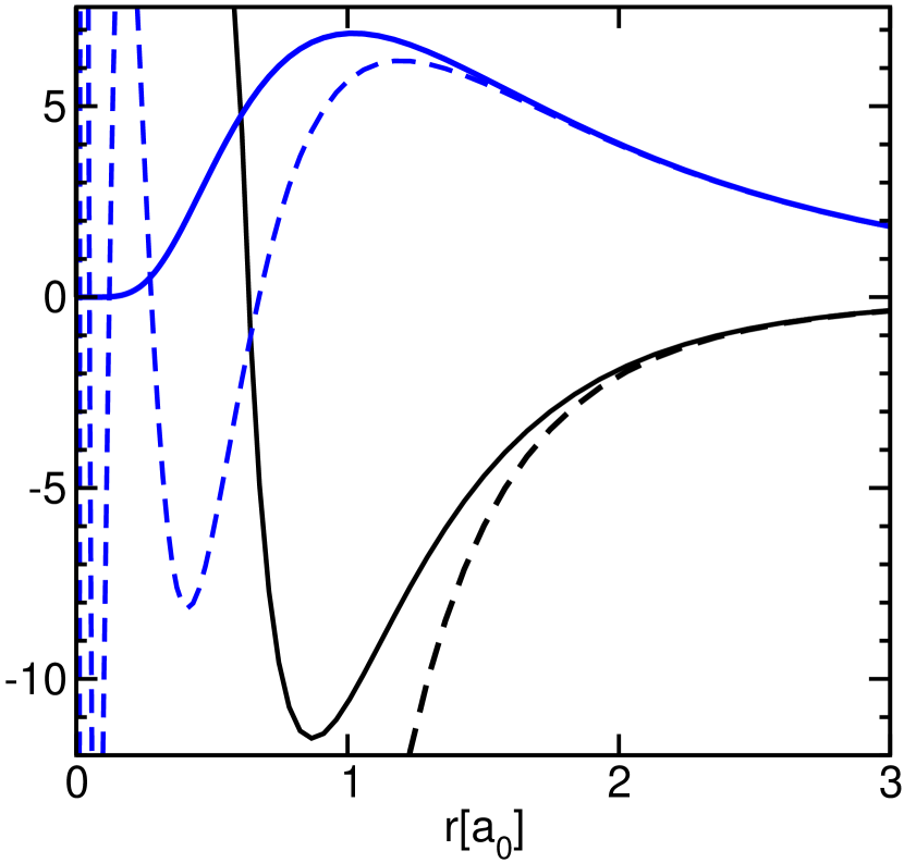
Figure 1: Node-less 6s wave functions shown as full lines for Gold (above) and its effective potential (below). The dashed functions are the full wave function and the full potential. The scale on the vertical axis is the potential value in Hartree.

The radial part of the wave function starts at the origin with a high power of $|\vec{r}|$. The depression of the wave function near the nucleus can be loosely attributed to the Pauli repulsion of the core electrons, that repel the valence electrons from the core region.

The leading power of the node-less wave functions near the origin is

$$\langle\vec{r}|u_{n}\rangle = \left(\frac{2m_{e}}{\hbar^{2}}\right)^{n-1}\frac{(2\ell+1)!!}{(2\ell-1+2n)!!(2n-2)!!}$$ (10)

$$\times|\vec{r}|^{\ell+2(n-1)}\textrm{e}^{-\lambda_{n}r}Y_{\ell,m}(\vec{r})(1+O(|\vec{r}|^{2}))\;.$$

The leading-order term is derived in appendix A. The exponential function with the yet unspecified parameter $\lambda_{n}$ has been added, because it provides a good description of the qualitative behavior of the wave function over a fairly wide region near the origin.

Eq. 10 shows that node-reduced partial waves start out at the origin with a increasingly high power, as $n$ is increased. We found it surprising that no trace of the nodal structure is left near the origin.

II.3 Construction of node-reduced wave functions

Now,we introduce energy-dependent partial waves via the differential equation

$$(H-E)|q_{n}(E)\rangle=-|u_{n-1}\rangle\;.$$ (11)

We will call them node-reduced partial waves, because their number of nodes is $n-1$ less than that of the regular partial wave $|\phi(E)\rangle$ at the same energy. This construction allows one to effectively remove the core states from the shape of the wave function and from the scattering properties.

The boundary conditions at the origin of the node-reduced partial waves are chosen analogously to those for $|u_{n}\rangle$, namely

$$\lim_{|\vec{r}|\rightarrow 0}\frac{q_{n}(E,\vec{r})}{u_{n}(\vec{r})}=1\;.$$ (12)

$|q_{1}(E)\rangle$ is identical to the regular energy-dependent partial wave $|\phi(E)\rangle$ with the normalization from Eq. 2.

Using $E=E_{n}$ and comparing Eq. 11 with Eq. 7, we obtain that the bound states of the node-reduced partial waves are the node-less wave functions defined before, i.e.

$$|q_{n}(E_{n})\rangle=|u_{n}\rangle\;.$$ (13)

The energy-dependent wave function $|\phi(E)\rangle$ can be reconstructed from the node-reduced wave function $|q_{n}(E)\rangle$ and the node-less bound states $|u_{n}\rangle$ by

$$|\phi(E)\rangle = \biggl{[}|q_{n}(E)\rangle+\sum_{m=1}^{n-1}|u_{m}\rangle\prod_{j=m}^{n-1}\frac{1}{E_{j}-E}\biggr{]}$$ (14)

$$\times\prod_{j=1}^{n-1}(E_{j}-E)\;.$$

Thus we obtained a partition of the wave function into a node-reduced part and a part related to the core wave functions, which is again expressed in terms of node-less wave functions.

As shown in appendix B, the node-reduced wave function can be expressed as difference

$$|q_{n+1}(E)\rangle=\left(|q_{n}(E)\rangle-|q_{n}(E_{n})\rangle\right)\frac{1}{E-E_{n}}$$ (15)

of two node-reduced wave functions $|q_{n}(E)\rangle$ with one additional node. According to Eq. 15, we can construct all $|q_{n}(E)\rangle$ from the energy-dependent partial wave $|\phi(E)\rangle$, if the latter is normalized such that the leading term at the origin remains energy-independent.

Specifically for the bound state energies, the node-reduced wave functions are related, as shown in appendix C, to the energy derivatives of other node-reduced wave functions.

$$|q_{n+j}(E_{n})\rangle=\frac{1}{j!}|q_{n}^{(j)}(E_{n})\rangle$$ (16)

where

$$|q^{(j)}_{n}(E)\rangle:=\partial_{E}^{j}|q_{n}(E)\rangle$$ (17)

is the $j$-th energy derivative of $|q_{n}(E)\rangle$.

Using Eq. 16, we find that the node-reduced wave functions are related to each other by a Taylor expansion about one bound state energy

$$|q_{n}(E)\rangle=\sum_{j=0}^{\infty}|q_{n+j}(E_{n})\rangle(E-E_{n})^{j}$$ (18)

II.4 Towards a nodal-theorem for node-reduced wave functions

Eq. 14 sheds some light on the question of the node-less-ness of the wave function $|u_{n}\rangle$:

We will show later, that the assumptions of the nodal theorem for the node-reduced wave functions is violated in the scattering region. Nevertheless, the assumptions are valid in the energy region of bound states. It is our hope that a variant of the nodal theorem can be found that holds for the entire energy region.

A nodal theorem for $|q_{n}(E)\rangle$ requires one to make the assumption that the node-less functions $|u_{m}\rangle$ with $m<n$ do not reach the outer boundary $|\vec{r}|=r_{x}$ for the node count. This assumption is reasonable for bound states of an atom if the outer boundary is chosen sufficiently far away.

With this assumption, the decomposition of the wave function in Eq. 14 shows that $|q_{n}(E)\rangle$ has bound states for all energies $E_{j}$ with $j\geq n$. At the lower bound states, that is for $j<n$ the node-less wave function $|q_{n}(E)\rangle$ does not have a node, but its contribution is removed by the energy-dependent factors in Eq. 14.

Under the same assumption, the regular nodal theoremCourant and Hilbert (1924) shows that nodes of the node-reduced partial waves at the outer bound move inward. Thus the number of nodes increases by one at each energy $E_{j}$ with $j\geq n$.

We can also exclude that nodes leave the interval at the center, because the leading order of the Taylor expansion about the origin is, according to Eq. 13, energy independent. If a node would migrate across the origin, the leading order of $|q(E)\rangle$ would change sign in contradiction to Eq. 13.

Two additional assumptions need to be made, namely that there is no pair-wise creation or annihilation of nodes within the interval, and that there are no accidental nodes of the node-reduced wave function $|q_{n}(E)\rangle$ at the bound state energies $E_{j}$ with $j<n$.

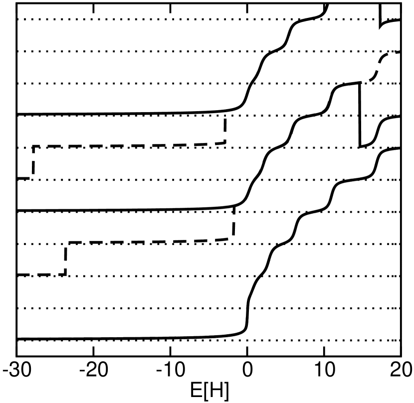
Figure 5: Phase shift function of Fe as defined by $N(E)+\frac{1}{2}-\frac{1}{\pi}\textrm{arctan}(\partial_{r}\ln(\phi(E,r)))$ as function of energy. $N(E)$ is the number of nodes within the radius at which the derivative of the wave function is taken. The phase shift functions have been displaced individually by integers for better comparison. The dotted lines mark integer values. The full lines are the phase shifts of the node-reduced partial wave and the dashed lines are those partial waves with the original nodal structure. From top to bottom, the s,p,d angular momentum channels are shown. The energy region between half-integer and the next integer value is the band region for this angular momentum channel. The steps of the dashed lines between -30 and -20 H reflect the 2s,2p shell and the one shortly below zero is the 3s,3p shell. The jumps in the high energy region reflect the annihilation of two nodes within the augmentation region.

Thus, for reasonable assumptions, these arguments show that the bound wave functions are free of nodes. In the scattering region at high energies though, the assumptions made are violated. Numerical calculations show violations of this nodal theorem, namely the pairwise formation of two nodes, in the high-energy region, which can be seen in Fig. 5.

As a consequence of the nodal theorem presented here, the number of nodes of the node-reduced wave function $|q_{n}(E)$ differs from that of the full wave functions by $n-1$ for energies above $E_{n}$ and it vanishes below.

II.5 Properties

II.5.1 Slater orbitals

In 1929 Slater suggested a simple form for node-less atomic orbitalsSlater (1930) of the form

$$\chi(\vec{r})=Ar^{n^{*}-1}\mathrm{e}^{-\frac{Z-s}{n^{*}a_{0}}r}\;,$$ (19)

where $n^{*}$ is an effective main quantum number, Z is the atomic number of the atom, $s$ is a screening constant, $a_{0}$ is the Bohr radius and $A$ is a normalization constant.

The guiding idea of Slater is related to ours, namely to exploit that the number of nodes is of only secondary importance for many of the chemical properties, if only the outer tail of the wave function is properly described. In this regard, our node-less functions can be considered an extension of Slater’s orbitals. In contrast to Slater’s orbitals our node-less functions contain, as a set, the complete information of the wave functions, at the cost that they do not have the simple analytical form of Slater’s orbitals.

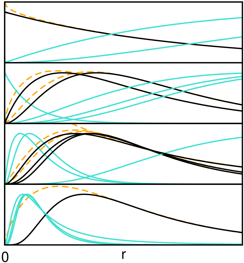
Figure 2: Node-less wave functions of the Fe atom and comparison with Slater orbitals as function of the distance from the center. Each graph shows in black the orbitals from one main quantum number (full black line) and the corresponding Slater orbital (orange dashed line). The orbitals of the neighboring main quantum numbers are show in (green, full lines). The wave functions are scaled to the same maximum value. The horizontal axis is scaled for each graph individually to make the shape similarity evident. The range of radii on the horizontal axis extend from the origin to 0.05, 0.35, 1.3, and 5 a₀, respectively from top to bottom.

The qualitative behavior and the similarity to Slater’s orbitals have been investigated by first by Thiemethieme03_diploma and FörstFörst (2004). The series of node-less functions is shown in Fig. 2.

Interesting to see is that the node-less 3d wave function of Fe is much closer in space to the 3s and 3p node-less wave functions than to the 4s wave function, to which it is energetically closer. It has been a general observation that the the node-less wave functions group according to their main quantum number into sets with similar range, and that these sets are well separated from those with a different main quantum number. With increasing atomic number, the wave functions with same main quantum number become even more similar as seen in Fig. 3.

The Slater orbitals, shown as dashed lines in Fig. 2, have been parameterized to reproduce the radial density maximum, i.e. the maximum of $r^{2}u_{n}^{2}(r)$, in value and position and the logarithmic derivative at a distance 1.5 times that of the density maximum. The tails of the wave function match fairly well, while there are deviations in the inner region. Compared to the Slater orbitals, which decay with a power time an exponential, the node-less wave functions have a simple exponential tail.

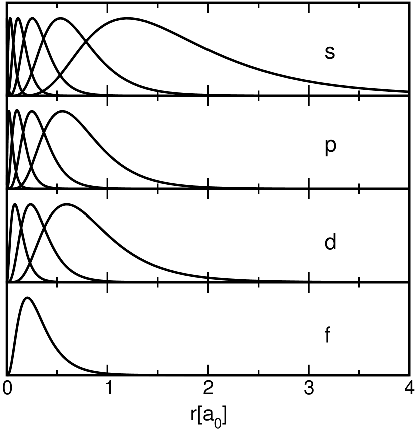
Figure 3: Node-less wave functions for Gold for s,p,d and f electrons from top to bottom. The wave functions are normalized to have identical maximum value

II.5.2 Pauli repulsion

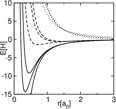
Figure 4: Effective potential including Pauli repulsion for the 3s3p3d shell (full) the 4s4p4d shell (dashed) and the 5s5p5d shell (dotted) of Fes²d⁶. For the shell with main quantum number 3 and 4, the effective potentials decrease with increasing angular momentum. For the 3d channel the effective potential equals the true potential.

One motivation for the node-less construction was to construct parameter-free pseudopotentials to be used for example to embed a quantum mechanical calculation into an environment described by a simpler theory. By inverting the Schrödinger equation for the node-less wave functions, one can construct an effective potential, that includes the effect of the Pauli repulsion. For a node-reduced wave function, which obeys Eq. 11, we obtain the potential with the Pauli repulsion by

$$v_{eff,n}(\vec{r})=E+\frac{\hbar^{2}\vec{\nabla}^{2}u_{n}(\vec{r})}{2mu_{n}(\vec{r})}\;.$$ (20)

The potential is semi-local, that is a different potential acts on each angular momentum channel. Here, only a specific angular momentum channel is considered.

The effective potential can also be constructed from the node-reduced partial waves, $|q_{n}(E)\rangle$, but this requires an energy below the first bound state to avoid poles in the potential resulting from the nodes in the wave function. The energy derivative of this potential provides an overlap operator, that, however, can also be obtained directly from the norm of the node-less wave functions as compared to the true nodal wave function.

In Fig. 4, the effective potentials are shown for the shells with main quantum number 3 to 5 for iron. The potentials become more repulsive with increasing angular momentum.

Interestingly, the potentials form groups with similar behavior characterized by the main quantum number. This implies that a semilocal potential constructed from node-less wave functions with the same main quantum number is best approximated by a local potential. Such choices will also lead to the most stable and transferable pseudopotentials: In the case of Fe, shown in the example, it is advisable to include the 3s and 3p electrons as valence electrons.

Atomic wave functions without nodes, such as 3d wave functions, are special, because they do not experience any Pauli repulsion, so that the effective potential is equal to the total potential. For atoms having wave functions without nodes in the valence shell, such as first-row elements, 3d transition-metal elements or lanthanides, the intrinsic non-locality as judged from our Pauli repulsion potentials is strongest. It is these elements for which the construction of pseudopotentials is most difficult.

Currently, we are using these effective potentials to construct tight-binding orbitals which will be discussed in a forthcoming paperbloechl_ntbo .

II.5.3 Scattering properties

The shape of the node-less functions makes them suitable helper functions for the construction of pseudo wave functions for the PAW method.

Pseudo wave functions shall be identical to the true wave functions in the bonding region. The s- and p- wave function of transition metal ions have their outmost nodes fairly close to the covalent radius. As a result a pseudo wave function follows the all electron wave function into the downswing towards the outermost node. The requirement of node-less-ness for the pseudo wave function requires a sharp turn outside the node and a large region with low amplitude. This sharp turn imposes large amplitudes in the pseudopotential causing stability and transferability problems. If the construction is such that the pseudo wave function follows the node-less wave function this problem is largely avoided.

A second difficulty of constructing pseudo wave function is to avoid artificial core-like states. They can be induced by the proximity to semi-core states that are excluded from the valence shell. Because the pole of the logarithmic wave function of these states may be noticeable, the pseudized wave functions try to reproduce this pole resulting in artificial undesired states. When the node-reduced wave functions are used as basis for the construction of the pseudo-potential, this problem is avoided.

II.5.4 Towards a systematic projector augmentation

In the PAW methodBlöchl (1994), the true Kohn-Sham wave functions $|\Psi\rangle$ are constructed as

$$|\Psi\rangle=|\tilde{\Psi}\rangle+\sum_{\alpha}\Bigl{(}|\varphi_{\alpha}\rangle-|\tilde{\varphi}_{\alpha}\rangle\Biggr{)}\langle\tilde{p}_{\alpha}|\tilde{\Psi}\rangle$$ (21)

from auxiliary wave functions $|\tilde{\Psi}\rangle$ by augmenting them with the difference of all-electron and auxiliary partial waves, $|\phi_{\alpha}\rangle$ and $|\tilde{\phi}_{\alpha}\rangle$ respectively. The coefficients are obtained using the projector functions $\langle\tilde{p}_{\alpha}|$, that obey a biorthogonality condition

$$\langle\tilde{p}_{\alpha}|\tilde{\phi}_{\beta}\rangle=\delta_{\alpha,\beta}$$ (22)

with the auxiliary partial waves.

Node-less wave functions guide us to a more systematic construction of the augmentation of the projector augmented wave method. So far, the mapping between all-electron and pseudo partial waves has been done for a selected grid of energiesBlöchl (1994). One difficulty is to ensure that the choice of auxiliary partial waves is consistent, that is to ensure that the augmentation leads to a converging series.

By inspecting some of the conventional pseudization schemes, we observed that the difference in shape between the resulting energy-dependent auxiliary partial waves $|\tilde{\phi}_{\alpha}\rangle$ and the node-reduced wave functions $|q_{n}(E_{\alpha})\rangle$ depends only weakly on energy. This suggests a new approach for choosing the projector augmentation.

We propose the following ansatz for the auxiliary partial waves, namely

$$|\tilde{\phi}(E)\rangle=|q_{n}(E)\rangle+|k\rangle\;,$$ (23)

where $|k\rangle$ is energy-independent function that is entirely localized in the augmentation region. A convenient way to choose $|k\rangle$ is to construct the pseudo partial wave with a conventional method for one single energy for each angular momentum and then to resolve Eq. 23 for $|k\rangle$.

Following the recipe of the PAW methodBlöchl (1994), one constructs raw, energy dependent projector functions via

$$|\tilde{p}^{\prime}(E)\rangle=\biggl{(}\frac{\hat{\vec{p}}^{2}}{2m_{e}}+\tilde{v}-E\biggr{)}|\tilde{\phi}(E)\rangle\;.$$ (24)

The auxiliary potential $\tilde{v}$ is a local potential, that is identical to the true potential beyond the augmentation region and smooth inside. The prime has been attached to the raw projector functions to distinguish them from the final projector functions obtained by enforcing the biorthogonalization Eq. 22.

Insertion of the Ansatz Eq. 23 into Eq. 24 results, with the help of Eq. 11, in

$$|\tilde{p}^{\prime}(E)\rangle = -|u_{n-1}\rangle+\left(\tilde{v}(\hat{\vec{r}})-v(\hat{\vec{r}})\right)|q_{n}(E)\rangle$$ (25)

$$+ \biggl{(}\frac{\hat{\vec{p}}^{2}}{2m_{e}}+\tilde{v}-E\biggr{)}|k\rangle\;.$$

Instead of using a grid of energies we can use the Taylor expansion of this expression in the energy about some value $E_{\nu}$.

$$|\tilde{p}^{\prime(j)}(E_{\nu})\rangle = \left[-|u_{n-1}\rangle+\biggl{(}\frac{\hat{\vec{p}}^{2}}{2m_{e}}+\tilde{v}-E_{\nu}\biggr{)}|k\rangle\right]\delta_{j,0}$$ (26)

$$-|k\rangle\delta_{j,1}+\left(\tilde{v}(\hat{\vec{r}})-v(\hat{\vec{r}})\right)|q_{n}^{(j)}(E_{\nu})\rangle\;,$$

where $|\tilde{p}^{\prime(j)}(E_{\nu})\rangle$ is the $j$-th energy derivative of $|\tilde{p}^{\prime}(E)\rangle$ at the energy $E_{\nu}$. Note, that the last term vanishes quickly with increasing $j$, because the difference of the potentials is concentrated in the inner region of the atom, while the radius, beyond which $|q^{(j)}_{n}\rangle$ becomes appreciable, rapidly shifts further out with each increasing $j$.

The Taylor expansion of the auxiliary partial waves defined in Eq. 23 is

$$|\tilde{\phi}^{(j)}(E_{\nu})\rangle=|q_{n}^{(j)}(E_{\nu})\rangle+|k\rangle\delta_{j,0}\;.$$ (27)

Finally, the biorthogonality condition is enforced either by a Gram-Schmidt like bi-orthogonalization or by inversion.

$$|\tilde{p}_{j}\rangle = \sum_{j^{\prime}}|\tilde{p}^{\prime(j^{\prime})}(E_{\nu})\rangle\biggl{(}\langle\tilde{\phi}^{(j)}(E_{\nu})|\tilde{p}^{\prime(j)}(E_{\nu})\rangle\biggr{)}^{-1}_{j^{\prime},j}$$

$$|\tilde{\varphi}_{j}\rangle = |\tilde{\phi}^{(j)}(E_{\nu})\rangle$$

$$|\varphi_{j}\rangle = |\phi^{(j)}(E_{\nu})\rangle\;.$$ (28)

Tests for this class of projector augmentation will be presented in a forthcoming paper.

III Conclusions

A set of functions has been presented that provides the description of the atomic bound and scattering wave functions without the obscuring nodal structure. An explicit transformation mediates between the original wave functions and what we call “node-less” or “node-reduced” wave functions.

This set of wave functions finds applications in the construction of pseudopotentials or the auxiliary partial waves in the PAW method. It provides an effective potential that describes the Pauli-repulsion of the core electrons without explicit orthogonalization. The node-less wave functions will be used to define tight-binding orbitals for the analysis of chemical binding or the calculation of correlated materials.

Acknowledgement: Financial support by the Deutsche Forschungsgemeinschaft through FOR 1346 is gratefully acknowledged.

Appendix A Power-series expansion at the origin

The behavior of the node-reduced wave functions at the origin is analyzed by the power-series expansion of the corresponding inhomogeneous differential equation Eq. 11. The radial part of the node-reduced wave function is represented as $q(E,r)=\sum_{j}a_{j}r^{\ell+j}$, that of the inhomogeneity as $u_{n-1}(r)=-\sum_{j}g_{j}r^{\ell+j}$ and the potential is expressed as

$$v(r)=-\frac{Ze^{2}}{4\pi\epsilon_{0}r}+\sum_{m=0}^{\infty}v_{m}r^{m}$$ (29)

The radial part of the differential equation Eq. 11 has the form

$$\Bigl{[}\frac{-\hbar^{2}}{2m_{e}}\left(\frac{1}{r}\partial^{2}_{r}r-\frac{\ell(\ell+1)}{r^{2}}\right)$$

$$-\frac{Ze^{2}}{4\pi\epsilon_{0}r}+\sum_{m=0}^{\infty}v_{m}r^{m}-E\Bigr{]}\sum_{j}a_{j}r^{\ell+j}=\sum_{j}g_{j}r^{\ell+j}$$

It results in the following recursion for the coefficients $a_{j}$.

$$a_{j} = \frac{2m_{e}}{-\hbar^{2}(2\ell+j+1)j}\biggl{[}\frac{Ze^{2}}{4\pi\epsilon_{0}}a_{j-1}$$ (30)

$$-\sum_{m=0}^{\infty}a_{j-m-2}(v_{m}-E\delta_{m,0})+g_{j-2}\biggr{]}$$

The regular solution of the homogeneous problem starts with $a_{0}$, i.e. $a_{j}=0$ for $j<0$. The irregular solution of the homogeneous problem starts with $a_{-2\ell-1}$, i.e. $a_{j}=0$ for $j<-2\ell-1$. For the inhomogeneous differential equation, we can add a solution of the homogenous problem, so that the leading term of the solution is determined by the inhomogeneity, given that the leading power of the inhomogeneity is higher than $r^{\ell}$. If the lowest-order term of the inhomogeneity is $g_{m}$, the lowest-order term of the wave function is of order $m+2$, i.e. $a_{j}=0$ for $j<m+2$.

$$a_{j}=-\frac{2m_{e}}{\hbar^{2}(2\ell+j+1)j}g_{j-2}$$ (31)

Thus the behavior at the origin is

$$\langle\vec{r}|q_{n}(E)\rangle = \left(\frac{2m_{e}}{\hbar^{2}}\right)^{n-1}\frac{(2\ell+1)!!}{(2\ell-1+2n)!!(2n-2)!!}$$ (32)

$$\times|\vec{r}|^{\ell+2(n-1)}Y_{\ell,m}(\vec{r})(1+O(|\vec{r}|))$$

Thus the leading power increases by two with increasing main quantum number, which describes the repulsion from the origin. The prefactor of the leading power is furthermore energy-independent.

Appendix B Recursion for energy dependent node-reduced wave functions

Here we show that $|q_{n}(E)\rangle$ for $n>1$ can be represented as difference between two functions $|q_{n-1}(E)\rangle$ at different energies by Eq. 15.

We start with a trial function $|f(E)\rangle$ defined by Eq. 15:

$$|f(E)\rangle:=\Bigl{(}|q_{n-1}(E)\rangle-|q_{n-1}(E_{n-1})\rangle\Bigr{)}\frac{1}{E-E_{n-1}}$$ (33)

and show that it satisfies all conditions for $|q_{n}(E)\rangle$, namely differential equation Eqs. 11 and boundary conditions Eq. 12.

Using Eq. 33, together with Eqs. 11 and 13 for the node-reduced functions $|q_{n-1}(E)\rangle$, we find

$$(H-E)|f(E)\rangle = |u_{n-1}\rangle$$ (34)

which is identical to the differential equation Eq. 11 for $|q_{n}(E)\rangle$.

The boundary conditions at the origin are defined by the admixture of the homogeneous solutions, that have the leading power $-\ell-1$ and $\ell$. Because the leading power of $|q_{n-1}(E)\rangle$ in $r$ is, due to Eq. 32, energy independent, and higher or equal to $r^{\ell}$, the leading power of $|f(E)\rangle$ is determined by the inhomogeneity. Thus the boundary behavior is determined directly by the differential equation, which is identical for $|f(E)\rangle$ and $|q_{n}(E)\rangle$

Since $|f(E)\rangle$ and $|q_{n}(E)\rangle$ obey the same inhomogeneous differential equation and the same boundary conditions, namely value and derivative at the origin, they are identical, which proves Eq. 15.

Appendix C Energy derivatives of node-reduced wave functions

Here, we show that the energy-derivatives of the node-reduced wave functions at the energy $E_{n}$ of a specific bound state are related by Eq. 16, namely

$$|q_{n+j}(E_{n})\rangle=\frac{1}{j!}|q^{(j)}_{n}(E_{n})\rangle$$ (35)

where the $q^{(j)}_{n}(E)$ is the $j$-th energy derivative of $|q_{n}(E)\rangle$.

We start with Eq. 15 for $|q_{n+1}(E)\rangle$ and insert the Taylor expansion for $|q_{n}(E)\rangle$ about $E_{n}$

$$|q_{n+1}(E)\rangle \stackrel{{\scriptstyle Eq.~{}\ref{eq:qsequence}}}{{=}} \frac{|q_{n}(E)\rangle-|q_{n}(E_{n})\rangle}{E-E_{n}}$$ (36)

$$= \sum_{j=1}^{\infty}\frac{1}{j!}|q^{(j)}_{n}(E_{n})\rangle(E-E_{n})^{j-1}$$

Term-by-term comparison with the Taylor expansion of $|q_{n+1}(E)\rangle$ on the left-hand side yields

$$|q^{(j)}_{n+1}(E_{n})\rangle = \frac{1}{j+1}|q^{(j+1)}_{n}(E_{n})\rangle$$ (37)

Successive application of Eq. 37 leads to the desired result, Eq. 35 respectively, Eq. 16.

References

- (1) Corresponding author: peter.bloechl@tu-clausthal.de
- Hohenberg and Kohn (1964) P. Hohenberg and W. Kohn, Phys. Rev. 136, B864 (1964).
- Kohn and Sham (1965) W. Kohn and L. J. Sham, Phys. Rev. 140, A1133 (1965).
- Topiol et al. (1977) S. Topiol, A. Zunger, and M. Ratner, Chem. Phys, Lett 49, 367 (1977).
- Hamann et al. (1979) D. R. Hamann, M. Schlüter, and C. Chiang, Phys. Rev. Lett 43, 1494 (1979).
- Slater (1937) J. Slater, Phys. Rev. 51, 846 (1937).
- Andersen (1975) O. K. Andersen, Phys. Rev. B 12, 3060 (1975).
- Blöchl (1994) P. E. Blöchl, Phys. Rev. B 50, 17953 (1994).
- Andersen and Jepsen (1984) O. K. Andersen and O. Jepsen, Phys. Rev. Lett 53, 2571 (1984).
- Melius and III (1974) C. F. Melius and W. A. G. III, Phys. Rev. A 10, 1528 (1974).
- Zunger and Ratner (1978) A. Zunger and M. A. Ratner, Chem. Phys. 30, 423 (1978).
- Zunger and Cohen (1978) A. Zunger and M. L. Cohen, Phys. Rev. B 18, 5449 (1978).
- (13) R. Schade, P.E. Blöchl, Th. Pruschke in preparation.
- Courant and Hilbert (1924) R. Courant and D. Hilbert, Methoden der Mathematischen Physik, vol. 1 (Springer, 1924).
- Slater (1930) J. C. Slater, Phys. Rev. 36, 57 (1930).
- (16) M. Thieme, Diploma thesis, Clausthal University of Technology, 2003.
- Först (2004) C. Först, Ph.D. thesis, Vienna University of Technology, Austria, and Clausthal University of Technology, Germany (2004).
- (18) P. Blöchl, in preparation.