Extensions of linear regression models based on set arithmetic for interval data

Abstract

Extensions of previous linear regression models for interval data are presented. A more flexible simple linear model is formalized. The new model may express cross-relationships between mid-points and spreads of the interval data in a unique equation based on the interval arithmetic. Moreover, extensions to the multiple case are addressed. The associated least-squares estimation problems are solved. Empirical results and a real-life application are presented in order to show the applicability and the differences among the proposed models.

keywords: multiple linear regression model; interval data; set arithmetic; least-squares estimation

1 Introduction

The statistical treatment of interval data is recently being considered extensively (see [1, 2, 3, 4, 5, 6]). Interval data are useful to model variables with uncertainty in their formalization, due to an imprecise observation or an inexact measurement, fluctuations, grouped data or censoring. Linear regression models for interval data have been previously analyzed (see [7, 8, 9, 10, 11, 12, 13, 14, 15]). Regression models with interval-valued explanatory variables and interval-valued response are considered. There are two main approaches to face these kinds of problems. One is based on fitting separate models for mid-points and spreads (see [13, 14]). This approach has not been considered under probabilistic assumptions on the population models, and inferential studies have not been developed yet. This is non-trivial, since the non-negativity constraints satisfied by the spread variables prevent the corresponding model to be treated as a classical linear regression. Thus, although the usual fitting techniques are used, the associated inferences are no longer valid. The second approach overcomes this difficulty by considering a model based on the set arithmetic (see [9, 11]). The least squares estimators are found as solutions of constrained minimization problems and inferential studies have been developed in [10] and [12], among others.

Extensions for the simple linear regression models within the framework of the work in [9] and [11] are developed. On one hand, a more flexible simple linear model is formalized. The previous regression functions model the response mid-points (respectively spreads) by means of the explanatory mid-points (respectively spreads). The new model is able to accommodate cross-relationships between mid-points and spreads in a unique equation based on the set arithmetic. As the model in [11], the new one is based on the so-called canonical decomposition of the intervals. On the other hand, extensions to the multiple case are addressed. Due to the essential differences of the model in [9] and those based on the canonical decomposition, two multiple models will be introduced. The least-squares (LS) estimation problems associated with the proposed regression models are solved. Some empirical results and a real-life application are presented in order to show the applicability and the differences among the proposed models.

The rest of the paper is organized as follows: In Section 2 some preliminary concepts about the interval framework are presented and several previous simple linear models based on the set arithmetic are revised. Extensions of those linear models are introduced in Sections 3, 4 and 5. The theoretical formalization and the associated LS estimation problems are addressed. In Section 6 the empirical performance and the practical applicability of the models are shown through some simulation studies and a real-life case-study. Finally, Section 7 includes some conclusions and future directions.

2 Preliminaries

The considered interval experimental data are elements belonging to the space $\mathcal{K_{\mathrm{c}}}(\mathbb{R})=\{[a_{1},a_{2}]:a_{1},a_{2}\in\mathbb{R},a_{1}\leq a_{2}\}$. Each interval $A\in\mathcal{K_{\mathrm{c}}}(\mathbb{R})$ can be parametrized in terms of its mid-point, $\textrm{mid}\ A=(\sup A+\inf A)/2$, and its spread, $\textrm{spr}\ A=(\sup A-\inf A)/2$. The notation $A=[\mathrm{mid}A\pm\mathrm{spr}A]$ will be used. An alternative representation for intervals is the so-called canonical decomposition, introduced in [11], given by $A=\mathrm{mid}A[1\pm 0]+\mathrm{spr}A[0\pm 1]$. It allows the consideration of the mid and spr components of $A$ separately within the interval arithmetic.

The Minkowski addition and the product by scalars form the natural arithmetic on $\mathcal{K_{\mathrm{c}}}(\mathbb{R})$. In terms of the (mid, spr)-representation these operations can be jointly expressed as

$$A+\lambda B=[(\mathrm{mid}A+\lambda\mathrm{mid}B)\ \pm\ (\mathrm{spr}A+|\lambda|\mathrm{spr}B)]$$

for any $A,B\in\mathcal{K_{\mathrm{c}}}(\mathbb{R})$ and $\lambda\in\mathbb{R}$. The space $(\mathcal{K_{\mathrm{c}}}(\mathbb{R}),+,\ldotp)$ is not linear but semilinear (or conical), due to the lack of symmetric element with respect to the addition. $\mathcal{K_{\mathrm{c}}}(\mathbb{R})$ can be identified with the cone $\mathbb{R}\times\mathbb{R}^{+}$ of $\mathbb{R}^{2}$. The expression $A+(-1)B$ generally differs from the natural difference $A-B$. If it exists $C=A-_{H}B\in\mathcal{K_{\mathrm{c}}}(\mathbb{R})$ verifying that $A=B+C$, $C$ is called Hukuhara difference between the pair of intervals $A$ and $B$. The interval $C$ exists iff $\mathrm{spr}B\leq\mathrm{spr}A$.

For every $A,B\in\mathcal{K_{\mathrm{c}}}(\mathbb{R})$, the $L_{2}$-type generic metric in [16] is defined as

$$d_{\theta}(A,B)=((\mathrm{mid}A-\mathrm{mid}B)^{2}+\theta\,(\mathrm{spr}A-\mathrm{spr}B)^{2})^{\frac{1}{2}}$$ (1)

for an arbitrary $\theta\in(0,\infty)$.

Given a probability space $(\Omega,\mathcal{}{A},P)$, the mapping $\emph{{x}}:\Omega\rightarrow\mathcal{K_{\mathrm{c}}}(\mathbb{R})$ is said to be a random interval iff $\mathrm{mid}\,\emph{{x}},\mathrm{spr}\,\emph{{x}}:\Omega\rightarrow\mathbb{R}$ are real random variables and $\mathrm{spr}\,\emph{{x}}\geq 0$. Random intervals will be denoted with bold lowercase letters, x, random interval-valued vectors will be represented by non-bold lowercase letters, $x$, and interval-valued matrices will be denoted with uppercase letters, $X$.

The expected value of x is defined in terms of the well-known Aumann expectation, which satisfies that

$$E(\emph{{x}})=[E(\mathrm{mid}\,\emph{{x}})\pm E(\mathrm{spr}\,\emph{{x}})],$$ (2)

whenever $\mathrm{mid}\,\emph{{x}},\mathrm{spr}\,\emph{{x}}\in L^{1}$. The variance of a random interval x can be defined as the usual Fréchet variance (see [17]) associated with the Aumann expectation in the metric space $(\mathcal{K_{\mathrm{c}}}(\mathbb{R}),d_{\theta})$, i.e.

$$\sigma^{2}_{\emph{{x}}}=E\Big{(}d_{\theta}^{2}(\emph{{x}},E(\emph{{x}}))\Big{)}\,=\sigma^{2}_{\textrm{mid}\emph{{x}}}+\theta\sigma^{2}_{\textrm{spr}\emph{{x}}},$$

whenever $\mathrm{mid}\,\emph{{x}},\mathrm{spr}\,\emph{{x}}\in L^{2}$. The conical structure of the space $\mathcal{K_{\mathrm{c}}}(\mathbb{R})$ entails some differences to define the usual covariance (see [18]). In terms of the $d_{\theta}$ metric it has the expression

$$\sigma_{\emph{{x}},\emph{{y}}}=\sigma_{\textrm{mid}\emph{{x}},\textrm{mid}\emph{{y}}}+\theta\sigma_{\textrm{spr}\emph{{x}},\textrm{spr}\emph{{y}}},$$

whenever those classical covariances exist. The expression $Cov(x,y)$ denotes the covariance matrix between two random interval-valued vectors $x=(\emph{{x}}_{1},\ldots,\emph{{x}}_{k})$ and $y=(\emph{{y}}_{1},\ldots,\emph{{y}}_{k})$.

Let $\emph{{x}},\emph{{y}}:\Omega\rightarrow\mathcal{K_{\mathrm{c}}}(\mathbb{R})$ be two random intervals. The basic simple linear model (see [8]) to relate two random intervals has the expression:

$$\emph{{y}}=b\emph{{x}}+\boldsymbol{\varepsilon}$$ (3)

with $b\in\mathbb{R}$ and $\boldsymbol{\varepsilon}:\Omega\rightarrow\mathcal{K_{\mathrm{c}}}(\mathbb{R})$ is an interval-valued random error such that $E[\boldsymbol{\varepsilon}|\emph{{x}}]=\Delta\in\mathcal{K_{\mathrm{c}}}(\mathbb{R})$. The LS estimation of (3) has been solved analytically by means of a constrained minimization problem in [9].

Model (3) only involves one regression parameter $b$ to model the dependency. Thus, it induces quite restrictive separate models for the mid and spr components of the intervals. Specifically, $\mathrm{mid}\emph{{y}}=b\mathrm{mid}\emph{{x}}+\mathrm{mid}\boldsymbol{\varepsilon}$ and $\mathrm{spr}\emph{{y}}=|b|\mathrm{spr}\emph{{x}}+\mathrm{spr}\boldsymbol{\varepsilon}$.

A more flexible linear model, called model M, has been introduced in [11]. It is defined in terms of the canonical decomposition as follows:

$$\emph{{y}}=b^{1}\mathrm{mid}\emph{{x}}\,[1\pm 0]+b^{2}\mathrm{spr}\emph{{x}}\,[0\pm 1]+\gamma\,[1\pm 0]+\boldsymbol{\varepsilon},$$ (4)

where $b^{1},b^{2}\in\mathbb{R}$ are the regression coefficients, $\gamma\in\mathbb{R}$ is an intercept term influencing the mid component of y and $\boldsymbol{\varepsilon}$ is a random interval error satisfying that $E[\boldsymbol{\varepsilon}|\emph{{x}}]=[-\delta,\delta]$, with $\delta\geq 0$. From (4) the linear relationships $\mathrm{mid}\emph{{y}}=b^{1}\mathrm{mid}\emph{{x}}+\gamma+\mathrm{mid}\boldsymbol{\varepsilon}$ and $\mathrm{spr}\emph{{y}}=|b^{2}|\mathrm{spr}\emph{{x}}+\mathrm{spr}\boldsymbol{\varepsilon}$ are transferred, where $b^{1}$ and $b^{2}$ may be different. The LS estimation leads to analytic expressions of the regression parameters of model M (see [11]). Confidence sets based on those estimators have been developed in [12].

3 A flexible simple linear regression model: the model $\mathrm{M}_{G}$

Following (4), the model $\mathrm{M}_{G}$ between x and y is defined as:

$$\noindent\emph{{y}}=b^{1}\mathrm{mid}\emph{{x}}[1\pm 0]+b^{2}\mathrm{spr}\emph{{x}}[0\pm 1]+b^{3}\mathrm{mid}\emph{{x}}[0\pm 1]+b^{4}\mathrm{spr}\emph{{x}}[1\pm 0]+\gamma[1\pm 0]+\boldsymbol{\varepsilon},$$ (5)

where $b^{i},\gamma\in\mathbb{R}$, $i=1,\ldots,4$ and $E(\boldsymbol{\varepsilon}|\emph{{x}})=[-\delta,\delta]\in\mathcal{K}_{c}(\mathbb{R})$, $\delta\geq 0$. The linear relationships for the mid and spr variables transferred from (5) are

$$\mathrm{mid}\emph{{y}}=b^{1}\mathrm{mid}\emph{{x}}+b^{4}\mathrm{spr}\emph{{x}}+\gamma+\mathrm{mid}\boldsymbol{\varepsilon}$$

and

$$\mathrm{spr}\emph{{y}}=|b^{2}|\mathrm{spr}\emph{{x}}+|b^{3}||\mathrm{mid}\emph{{x}}|+\mathrm{spr}\boldsymbol{\varepsilon}.$$

Thus, both variables $\mathrm{mid}\emph{{y}}$ and $\mathrm{spr}\emph{{y}}$ are modelled from the complete information provided by the independent random interval x, characterized by the random vector $(\mathrm{mid}\emph{{x}},\mathrm{spr}\emph{{x}})$.

For a simpler notation, the random intervals defined from x are denoted by $\emph{{x}}^{M}$, $\emph{{x}}^{S}$, $\emph{{x}}^{C}$ and $\emph{{x}}^{R}$, in the same order as they appear in (5). Thus, the model $\mathrm{M}_{G}$ is equivalently expressed as:

$$\emph{{y}}=b^{1}\ \emph{{x}}^{M}+b^{2}\ \emph{{x}}^{S}+b^{3}\ \emph{{x}}^{C}+b^{4}\ \emph{{x}}^{R}+\gamma[1\pm 0]+\boldsymbol{\varepsilon}.$$

Moreover, in order to unify the notation for the estimation problems of the different linear models, the real interval $\Delta=[\gamma-\delta,\gamma+\delta]$ is defined. Then, the regression function associated with the model $\mathrm{M}_{G}$ can be written as:

$$E(\emph{{y}}|\emph{{x}})=b^{1}\ \emph{{x}}^{M}+b^{2}\ \emph{{x}}^{S}+b^{3}\ \emph{{x}}^{C}+b^{4}\ \emph{{x}}^{R}+\Delta.$$ (6)

Since $\emph{{x}}^{S}=-\emph{{x}}^{S}$ and $\emph{{x}}^{C}=-\emph{{x}}^{C}$, the model $\mathrm{M}_{G}$ always admits four equivalent expressions. This property allows the simplification of the estimation process, because it is possible to search only for non-negative estimates of the parameters $b^{2}$ and $b^{3}$.

Given a random sample $\{\left(\emph{{x}}_{j},\emph{{y}}_{j}\right)\}_{j=1}^{n}$ obtained from two random intervals $(\emph{{x}},\emph{{y}})$ verifying (5), the LS estimation of the parameters $(b^{1},b^{2},b^{3},b^{4},\Delta)$ in (6) consists in minimizing

$$\frac{1}{n}\sum_{i=1}^{n}d_{\theta}^{2}(\emph{{y}}_{i},a\emph{{x}}_{i}^{M}+b\emph{{x}}_{i}^{S}+c\emph{{x}}_{i}^{C}+d\emph{{x}}_{i}^{R}+C)$$ (7)

over $(a,b,c,d,C)\in\mathbb{R}^{4}\times\mathcal{K}_{c}(\mathbb{R})$. However, since from equation (5), $\boldsymbol{\varepsilon}_{i}=\emph{{y}}_{i}-_{H}(b^{1}\emph{{x}}_{i}^{M}+b^{2}\emph{{x}}_{i}^{S}+b^{3}\emph{{x}}_{i}^{C}+b^{4}\emph{ {x}}_{i}^{R})$, (7) must be optimized over a suitable feasible set assuring the existence of the sample residuals, i.e., the corresponding Hukuhara differences. Note that

$$\mathrm{spr}(a\emph{{x}}_{i}^{M}+b\emph{{x}}_{i}^{S}+c\emph{{x}}_{i}^{C}+d\emph{{x}}_{i}^{R})=|b|\mathrm{spr}\emph{{x}}_{i}+|c||\textrm{mid}\emph{{x}}_{i}|$$

for all $i=1,\ldots,n$ and $b^{2}$ and $b^{3}$ can be assumed to be non-negative. Then, taking into account the condition guaranteeing the existence of the Hukuhara difference, the feasible set can be expressed as

$$\Gamma_{G}=\{(b,c)\in[0,\infty)\times[0,\infty):b\ \mathrm{spr}\emph{{x}}_{i}+c\ |\textrm{mid}\emph{{x}}_{i}|\leq\mathrm{spr}\emph{{y}}_{i},\forall i=1,\ldots,n\}.$$ (8)

If $(\widehat{b^{1}},\widehat{b^{2}},\widehat{b^{3}},\widehat{b^{4}})\in\mathbb{R}^{4}$ denotes a feasible estimate, then the interval parameter $\Delta$ can be directly estimated by

$$\widehat{\Delta}=\overline{\emph{{y}}}-_{H}\left(\widehat{b^{1}}\overline{\emph{{x}}^{M}}+\widehat{b^{2}}\overline{\emph{{x}}^{S}}+\widehat{b^{3}}\overline{\emph{{x}}^{C}}+\widehat{b^{4}}\overline{\emph{ {x}}^{R}}\right).$$

As a result, the LS minimization problem is

$$\min_{{\small\begin{array}[]{c}(a,d)\in\mathbb{R}^{2}\\ (b,c)\in\Gamma_{G}\end{array}}}\frac{1}{n}\sum_{i=1}^{n}d_{\theta}^{2}\Big{(}\emph{{y}}_{i}-_{H}(a\emph{{x}}_{i}^{M}+b\emph{{x}}_{i}^{S}+c\emph{{x}}_{i}^{C}+d\emph{ {x}}_{i}^{R}),\overline{\emph{{y}}}-_{H}(a\overline{\emph{{x}}^{M}}+b\overline{\emph{{x}}^{S}}+c\overline{\emph{ {x}}^{C}}+d\overline{\emph{{x}}^{R}})\Big{)}.$$ (9)

The problem (9) can be solved separately for $(a,d)$ and $(b,c)$. The minimization over $(a,d)$ is done without restrictions and it leads to the following analytic estimators of $(b^{1},b^{4})$ in the model $\mathrm{M}_{G}$:

$$(\widehat{b^{1}},\widehat{b^{4}})^{t}=S_{1}^{-1}z_{1}.$$ (10)

Here $z_{1}=(\widehat{\sigma}_{\emph{{x}}^{M},\emph{{y}}},\widehat{\sigma}_{\emph{{x}}^{R},\emph{{y}}})^{t}$ and $S_{1}$ corresponds to the sample covariance matrix of the interval-valued random vector $(\emph{{x}}^{M},\emph{{x}}^{R})$.

The minimization for $(b,c)$ is performed over the feasible set $\Gamma_{G}$, which is nonempty, closed and convex. The objective function to be minimized over $(b,c)$ can be expressed as the globally convex function

$$g(b,c)=(b)^{2}\ \widehat{\sigma}^{2}_{\emph{{x}}^{S}}+(c)^{2}\ \widehat{\sigma}^{2}_{\emph{{x}}^{C}}+2\ b\ c\ \widehat{\sigma}_{\emph{{x}}^{S},\emph{{x}}^{C}}-2\ b\ \widehat{\sigma}_{\emph{{x}}^{S},\emph{{y}}}-2\ c\ \widehat{\sigma}_{\emph{{x}}^{C},\emph{{y}}}.$$ (11)

If the global minimum of the function $g$ is so that $(b^{*},c^{*})^{t}\notin\Gamma_{G}$, then the local minimum of $g$ over $\Gamma_{G}$ is unique, and it is located on the boundary of $\Gamma_{G}$. The boundary of $\Gamma_{G}$, denoted by $\mathrm{fr}(\Gamma_{G})$, verifies that

$$\mathrm{fr}(\Gamma_{G})=L_{1}\cup L_{2}\cup L_{3}\ ,$$ (12)

where $L_{i}$, $i=1,2,3$ are the following sets:

• $L_{1}=\left\{(0,c)\,|\,0\leq c\leq r_{0}=\min_{i=1,\ldots,n}\frac{\mathrm{spr}\emph{{y}}_{i}}{|\mathrm{mid}\emph{{x}}_{i}|}\right\}$.

• $L_{3}=\left\{(b,0)\,|\,0\leq b\leq s_{0}=\min_{i=1,\ldots,n}\frac{\mathrm{spr}\emph{{y}}_{i}}{\mathrm{spr}\emph{{x}}_{i}}\right\}$.

• $L_{2}=\left\{(b,\min_{k=1\ldots n}\{-u_{k}b+v_{k}\})\,|\,0\leq b\leq s_{0}\right\}$, with
  

  $$u_{k}=\frac{\mathrm{spr}\emph{{x}}_{k}}{|\mathrm{mid}\emph{{x}}_{k}|}\ \mbox{ and }\ v_{k}=\frac{\mathrm{spr}\emph{{y}}_{k}}{|\mathrm{mid}\emph{{x}}_{k}|}\textrm{ for all }k=1,\ldots,n.$$

The set $L_{2}$ is composed on several straight segments from some of the straight lines $\{l_{k}:c=-u_{k}b+v_{k}\}_{k=1}^{n}$. If $|\mathrm{mid}\emph{{x}}_{k}|=0$ for any $k\in\{1,\ldots,n\}$, then the corresponding straight line is $b=\mathrm{spr}\emph{{y}}_{k}/\mathrm{spr}\emph{{x}}_{k}$ for $\mathrm{spr}\emph{{x}}_{k}\neq 0$. Thus, it is a vertical line, which could take part in $L_{2}$ only if $\mathrm{spr}\emph{{y}}_{k}/\mathrm{spr}\emph{{x}}_{k}=s_{0}$. Moreover, if $\mathrm{spr}\emph{{x}}_{k}=0$ too, then the sample interval $\emph{{x}}_{k}$ is reduced to the real value $\emph{{x}}_{k}=0$, so it does not take part in the construction of $\Gamma_{G}$. In Figure 1 the feasible set and its boundary in a practical example are illustrated graphically. The sample data corresponds to a real-life example (see Section 6.1).

Figure 1: $\Gamma_{G}$ for the sample data in Table 1

In order to find the exact solution of $\min_{(b,c)\in\Gamma_{G}}g(b,c)$ the global minimum of $g$ should be computed and, if needed, the local minimum over $L_{i},i=1,2,3$.

The asymptotic time complexity of the algorithm is $0(nt)$, where $t$ is the number of lines in $\{l^{k}\}_{k=1}^{n}$ taking part in $\mathrm{fr}(\Gamma_{G})$. The straight lines in $\{l_{k}:c=-u_{k}b+v_{k}:k\neq(v),(h)\}_{k=1}^{n}$ such that $-u_{k}b_{(v,h)}+v_{k}>c_{(v,h)}$ do not take part on the construction of $\mathrm{fr}(\Gamma_{G})$. Thus, they can be ignored from Step 5 to the end of the algorithm. However, for practical examples with moderate sample sizes $n$, this reduction will result in a negligible improvement on the computational efficiency of the algorithm.

4 The multiple basic linear regression model

Let y be a response random interval and let $\emph{{x}}_{1},\emph{{x}}_{2},\ldots,\emph{{x}}_{k}$ be $k$ explanatory random intervals. The multiple basic linear regression model (MBLRM) extending (3) is formalized as:

$$\emph{{y}}=x^{t}b+\boldsymbol{\varepsilon}$$ (13)

being $x=(\emph{{x}}_{1},\emph{{x}}_{2},\ldots,\emph{{x}}_{k})^{t}$, $b=(b_{1},b_{2},\ldots,b_{k})^{t}\in\mathbb{R}^{k}$ and $\boldsymbol{\varepsilon}$ an random interval-valued error such that $E(\boldsymbol{\varepsilon}|x)=\Delta\in\mathcal{K_{\mathrm{c}}}(\mathbb{R})$. The associated regression function is $E(\emph{{y}}|\emph{{x}}_{1}=x_{1},\ldots,\emph{{x}}_{k}=x_{k})=x^{t}b+\Delta$. Thereafter, the second-order moments of the random intervals involved in the linear model (13) are assumed to be finite, and the variances strictly positive. If the mids and spreads of the explanatory intervals are not degenerated, then (13) is unique. The following separate models are transferred:

$$\left.\begin{array}[]{c}\mathrm{mid}\emph{{y}}=\mathrm{mid}(x^{t})\,b+\mathrm{mid}\,\boldsymbol{\varepsilon},\textrm{ and }\\ \mathrm{spr}\emph{{y}}=\mathrm{spr}(x^{t})\,|b|+\mathrm{spr}\,\boldsymbol{\varepsilon}.\end{array}\right.$$ (14)

The mid variables relates through a standard (real-valued) multiple linear model, but this is not the case for the spreads, due to the non-negative restrictions.

Let $\{\left(\emph{{y}}_{j},\emph{{x}}_{i,j}\right):i=1,\ldots,k,j=1,\ldots,n\}$ be a simple random sample of size $n$ obtained from y and $x=(\emph{{x}}_{1},\ldots,\emph{{x}}_{k})$ verifying (13). Then,

$$y=Xb+\varepsilon,$$ (15)

where $y=(\emph{{y}}_{1},\ldots,\emph{{y}}_{n})^{t}$, $X$ is the $(n\times k)$-interval-valued matrix such that $X_{j,i}=\emph{{x}}_{i,j}$, and $\varepsilon=(\boldsymbol{\varepsilon}_{1},\ldots,\boldsymbol{\varepsilon}_{n})^{t}$ fulfils $E[\varepsilon|X]=1^{n}\Delta$, $1^{n}$ denoting the ones’ vector in $\mathbb{R}^{n}$. The LS estimation consists in finding $\widehat{b}$ and $\widehat{\Delta}$ minimizing the objective function:

$$\min_{d\in\mathbb{R}^{k},C\in\mathcal{K_{\mathrm{c}}}(\mathbb{R})}d_{\theta}^{2}(y,Xd+1^{n}C)\ ,$$ (16)

constrained to the existence of the residuals $\widehat{\varepsilon}=y-_{H}X\widehat{b}$. If $\widehat{b}\in\Gamma=\{a\in\mathbb{R}^{k}:y-_{H}Xa\in\mathcal{K_{\mathrm{c}}}(\mathbb{R})^{k}\}$, then the optimum value over $C$ is attained at

$$\widehat{\Delta}=\overline{\emph{{y}}}-_{H}\overline{x^{t}}\widehat{b}.$$ (17)

Extending directly the estimation method in [9] would lead to a computationally unfeasible combinatorial problem. For that, a non-optimal stepwise algorithm has been proposed. However, that may be offset by estimating separately the absolute value of $\widehat{b}$ and its sign. Note that $\widehat{b}=|\widehat{b}|\circ sign(\widehat{b})$, and from (14), $sign(\widehat{b})$ is only determined by the sign of the relationship between the mid-points. Then, $sign(\widehat{b})_{i}=sign(\widehat{Cov}(\textrm{mid}\emph{{y}},\textrm{mid}x_{i}))$ and $|\widehat{b}|$ can be obtained as the solution of

$$\min_{a\in\Gamma,a\geq 0}d_{\theta}^{2}(y,X(a\circ sign(\widehat{b}))+1^{n}\widehat{\Delta}).$$ (18)

The feasible set $\Gamma^{\prime}=\Gamma\cap(\mathbb{R}^{k})^{+}$ in (18) can be expressed as

$$\Gamma^{\prime}=\{d\in(\mathbb{R}^{k})^{+}:(\textrm{spr}X)d\leq\textrm{spr}y\}.$$ (19)

A more operative expression for the objective function in (18) is:

$$d_{\theta}^{2}(y,X(a\circ sign(\widehat{b}))+1^{n}\widehat{\Delta}) = (v_{m}-F_{m}^{\prime}\,a)^{t}(v_{m}-F_{m}^{\prime}\,a)$$ (20)

$$+\theta(v_{s}-F_{s}^{\prime}\,a)^{t}(v_{s}-F_{s}^{\prime}\,a),$$

where $v_{m}=\mathrm{mid}y-\overline{\mathrm{mid}\emph{{y}}}1^{n}\in\mathbb{R}^{n}$, $v_{s}=\mathrm{spr}y-\overline{\mathrm{spr}\emph{{y}}}1^{n}\in\mathbb{R}^{n}$, $F_{m}=(\mathrm{mid}X-1^{n}(\overline{\mathrm{mid}x^{t}}))$, $F_{s}=\mathrm{spr}X-1^{n}(\overline{\mathrm{spr}x^{t}})$, $F_{m}^{\prime}=F_{m}\textrm{diag}(sign(\widehat{b})_{1},\ldots,sign(\widehat{b})_{k})\in\mathbb{R}^{n\times k}$, $F_{s}^{\prime}=F_{s}\textrm{diag}(sign(\widehat{b})_{1},\ldots,sign(\widehat{b})_{k})\in\mathbb{R}^{n\times k}$ and $a\in\mathbb{R}^{k}$. Since the optimization problem consists in minimizing a quadratic expression with inequality linear constraints, Karush-Kuhn-Tucker (KKT) conditions guarantee the existence of solution and it can be found by using a standard software.

5 The multiple flexible linear regression model

From (5), a multiple flexible linear regression model (MFLRM) can be defined as:

$$\emph{{y}}=\mathrm{mid}\,x^{t}\,[1\pm 0]\,b^{1}+\mathrm{spr}\,x^{t}\,[0\pm 1]\,b^{2}+\mathrm{mid}\,x^{t}\,[0\pm 1]\,b^{3}+\mathrm{spr}\,x^{t}\,[1\pm 0]\,b^{4}+\boldsymbol{\varepsilon}\ ,$$ (21)

where $b^{1},b^{2},b^{3},b^{4}\in\mathbb{R}^{k}$ and $E(\boldsymbol{\varepsilon}|x^{t})=\Delta\in\mathcal{K_{\mathrm{c}}}(\mathbb{R})$. Equivalently (21) can be written as:

$$\emph{{y}}=x^{M}\,b^{1}+x^{S}\,b^{2}+x^{C}\,b^{3}+x^{R}\,b^{4}+\boldsymbol{\varepsilon},$$ (22)

or, in matrix notation, as:

$$\emph{{y}}=X^{Bl}\,B+\boldsymbol{\varepsilon}\ ,$$ (23)

where $X^{Bl}=(x^{M}|x^{S}|x^{C}|x^{R})\in\mathcal{K_{\mathrm{c}}}(\mathbb{R})^{1\times 4k}$ and $B=((b^{1})^{t}|(b^{2})^{t}|(b^{3})^{t}|(b^{4})^{t})^{t}\in\mathbb{R}^{4k\times 1}$. The values $b^{2}$ and $b^{3}$ can be assumed to be non-negative without loss of generality since $x^{S}=-x^{S}$ and $x^{C}=-x^{C}$.

The separate linear relationships for the mid and spr components of the intervals transferred from (21) are

$$\mathrm{mid}\,\emph{{y}}=\mathrm{mid}\,(x^{t})\,b^{1}+\mathrm{spr}\,(x^{t})\,b^{4}+\mathrm{mid}\,\boldsymbol{\varepsilon}\ \mathrm{,and}$$ (24)

$$\mathrm{spr}\,\emph{{y}}=\mathrm{spr}\,(x^{t})\,b^{2}+|\mathrm{mid}\,(x^{t})|\,b^{3}+\mathrm{spr}\,\boldsymbol{\varepsilon}.$$ (25)

Let $\{\left(\emph{{y}}_{j},\emph{{x}}_{i,j}\right):i=1,\ldots,k,j=1,\ldots,n\}$ be a simple random sample obtained from the random intervals $(\emph{{y}},\emph{{x}}_{1},\ldots,\emph{{x}}_{k})$ verifying (21). Then,

$$y=X^{M}\,b^{1}+X^{S}\,b^{2}+X^{C}\,b^{3}+X^{R}\,b^{4}+\varepsilon\ ,$$

where $y=(\emph{{y}}_{1},\ldots,\emph{{y}}_{n})$, $\varepsilon=(\boldsymbol{\varepsilon}_{1},\ldots,\boldsymbol{\varepsilon}_{n})$ such that $E(\varepsilon|x)=1^{n}\Delta$, $(X^{M})_{i,j}=\mathrm{mid}\emph{{x}}_{i}[1\pm 0]$ and $X^{S},X^{C}$ and $X^{R}$ are analogously defined. It can be equivalently expressed in a matrix form as

$$y=X^{ebl}B+\varepsilon\ ,$$ (26)

where $X^{ebl}=(X^{M}|X^{S}|X^{C}|X^{R})\in\mathcal{K_{\mathrm{c}}}(\mathbb{R})^{n\times 4k}$ and $B$ as in (23).

The LS estimation searches for $\widehat{B}$ and $\widehat{\Delta}$ minimizing $\displaystyle d_{\theta}^{2}(y,X^{ebl}A+1^{n}C)$ for $A\in\mathbb{R}^{4k\times 1}$ and $C\in\mathcal{K}_{c}(\mathbb{R})$. The constraints to assure the existence of the residuals are:

$$\mathrm{spr}\,X\,\widehat{b^{2}}+|\mathrm{mid}\,X|\,\widehat{b^{3}}\leq\mathrm{spr}\,y.$$ (27)

The estimation of $B$ and $\Delta$ can be solved separately. If $\widehat{B}$ verifies (27), then the minimum value of $d_{\theta}^{2}(y,X^{ebl}\widehat{B}+1^{n}C)$ over $C\in\mathcal{K}_{c}(\mathbb{R})$ is attained at $\widehat{\Delta}=\overline{\emph{{y}}}-_{H}\overline{X^{Bl}}\widehat{B}$. The objective function can then be written as

$$d_{\theta}^{2}(y,X^{ebl}A+1^{n}\widehat{\Delta})=(v_{m}-F_{m}A_{m})^{t}(v_{m}-F_{m}A_{m})+\theta\,(v_{s}-F_{s}A_{s})^{t}(v_{s}-F_{s}A_{s})\ ,$$

where $v_{m},v_{s}\in\mathbb{R}^{n},F_{m},\,F_{s}\in\mathbb{R}^{n\times 2k}$ are defined as in (20), $A_{m}=((a^{2})^{t}|(a^{3})^{t})^{t}\in\mathbb{R}^{2k}$ are the coefficients affecting the mids and $A_{s}=((a^{1})^{t}|(a^{4})^{t})\in\mathbb{R}^{2k}$ the coefficients affecting the spreads, with $a^{l}\in\mathbb{R}^{k}$, $l=1,\ldots,4$.

Therefore, the computation of the LS estimator $\widehat{B}$ for the regression parameter $B$ in (23) is solved through the constrained optimization problem by KKT conditions:

$$\min_{A_{s}\in\mathbb{R}^{2k},A_{m}\in\Gamma_{2}}(v_{m}-F_{m}A_{m})^{t}(v_{m}-F_{m}A_{m})+\theta\,(v_{s}-F_{s}A_{s})^{t}(v_{s}-F_{s}A_{s})\ ,$$ (28)

with

$$\Gamma_{2}=\{(a^{2},a^{3})\in[0,\infty)^{k}\times[0,\infty)^{k}:\mathrm{spr}\,X\,a^{2}+|\mathrm{mid}\,X|\,a^{3}\leq\mathrm{spr}\,y\}.$$ (29)

Note that the extension of the linear regression model M developed in [11] to the multiple case is directly achieved from (21), taking $b^{3}=(0,\ldots,0)$ and $b^{4}=(0,\ldots,0)$.

6 Empirical results

6.1 Application to a real-life example

A real-life example concerning the relationship between the daily fluctuations of the systolic and diastolic blood pressures and the pulse rate over a sample of patients in the Hospital Valle del Nalón, in Spain, is considered (previously explored in [11, 8, 9]). The metric $d_{1/3}$ is employed, and the optimization algorithm quadprog to solve the estimation of the multiple models (13) and (21) is run.

Let y, $\emph{{x}}_{1}$ and $\emph{{x}}_{2}$ the fluctuation of the diastolic blood pressure of a patient over a day, the fluctuation of the systolic blood pressure over the same day, and the pulse range variation over the same day, respectively. Data in Table 1 correspond to a sample data of $59$ patients from $(\emph{{y}},\emph{{x}}_{1},\emph{{x}}_{2})$.

From the sample data provided in Table 1, the estimated model $\mathrm{M}_{G}$ for y and $\emph{{x}}_{1}$ is

$$\widehat{\emph{{y}}}=0.5383\emph{{x}}_{1}^{M}+0.2641\emph{{x}}_{1}^{S}-0.4412\emph{{x}}_{1}^{R}+[4.249,35.254].$$ (30)

The value of determination coefficient $R^{2}$ (defined as the proportion of explained variability) associated with this estimated model is $0.6857$.

The estimated model (13) for y and $(\emph{{x}}_{1},\emph{{x}}_{2})$ from the data set in Table 1 has the expression:

$$\widehat{\emph{{y}}}=0.4094\emph{{x}}_{1}+0.0463\emph{{x}}_{2}+[10.3630,29.5168].$$ (31)

The value of the determination coefficient is in this case $R^{2}=0.4221$.

The linear relationship between y and $(\emph{{x}}_{1},\emph{{x}}_{2})$ can be also estimated more naturally by means of the MFLRM. The estimation of the model (21) leads to the expression:

$$\widehat{\emph{{y}}} = 0.5435\,\emph{{x}}_{1}^{M}+0.0190\,\emph{{x}}_{2}^{M}+0.2588\,\emph{{x}}_{1}^{S}+0.1685\,\emph{{x}}_{2}^{S}-0.4446\,\emph{{x}}_{1}^{R}$$ (32)

$$+0.1113\,\emph{ {x}}_{2}^{R}+[3.2032,27.8373]\ ,$$

with $R^{2}=0.7922$.

The highest value of $R^{2}$ is achieved for (32), which agrees with the fact that MFLRM is the most flexible regression among the linear models that have been developed. The difference in the $R^{2}$ between this multiple model and the simple one in (30) is due to the inclusion of the pulse rate variable $\emph{{x}}_{2}$ in the prediction of y. However, this difference is not large, which indicates that the pulse rate has low explanatory power. The smallest value of $R^{2}$ corresponds to (31). It indicates that the multiple basic model is too restrictive to relate these physical magnitudes.

6.2 Simulation results

The empirical performance of the regression estimates for each linear model is investigated by means of some simulations. Three independent random intervals $\emph{{x}}_{1},\emph{{x}}_{2},\emph{{x}}_{3}$ and an interval error $\boldsymbol{\varepsilon}$ will be considered. Let $\mathrm{mid}\,\emph{{x}}_{1}\sim\mathcal{N}(1,2)$, $\mathrm{spr}\,\emph{{x}}_{1}\sim\mathcal{U}(0,10)$, $\mathrm{mid}\,\emph{{x}}_{2}\sim\mathcal{N}(2,1)$, $\mathrm{spr}\,\emph{{x}}_{2}\sim\mathcal{X}_{4}^{2}$, $\mathrm{mid}\,\emph{{x}}_{\,3}\sim\mathcal{N}(1,3)$, $\mathrm{spr}\,\emph{{x}}_{\,3}\sim\mathcal{U}(0,5)$, $\mathrm{mid}\,\boldsymbol{\varepsilon}\sim\mathcal{N}(0,1)$ and $\mathrm{spr}\,\boldsymbol{\varepsilon}\sim\mathcal{X}_{1}^{2}$. Different linear expressions with the investigated structures will be considered.

• Model $M_{1}$: According to the multiple basic linear model presented in (13), y it is defined by the expression:

  $$\emph{{y}}=2\emph{{x}}_{1}-5\emph{{x}}_{2}-\emph{{x}}_{3}+\varepsilon.$$ (33)

• Model $M_{2}$: A simple linear relationship in terms of the model $\mathrm{M}_{G}$ in (5) is defined by considering only $\emph{{x}}_{1}$ as independent interval for modelling y through the expression:

  $$\emph{{y}}=-2\emph{{x}}_{1}^{M}+2\emph{{x}}_{1}^{S}+\emph{{x}}_{1}^{C}+0.5\emph{ {x}}_{1}^{R}+\varepsilon.$$ (34)

• Model $M_{3}$: A multiple flexible linear regression model following (21) is defined as:

  y $$= -2\emph{{x}}_{1}^{M}+5\emph{{x}}_{2}^{M}-\emph{{x}}_{3}^{M}+2\emph{{x}}_{1}^{S}+2\emph{{x}}_{2}^{S}+\emph{{x}}_{3}^{S}+\emph{{x}}_{1}^{C}+\emph{{x}}_{2}^{C}+3\emph{{x}}_{3}^{C}$$ (35)

  $$+0.5\emph{{x}}_{1}^{R}+\emph{{x}}_{2}^{R}-3\emph{{x}}_{3}^{R}+\varepsilon.$$

From each linear model $l=10,000$ random samples has been generated for different sample sizes $n$. The estimates of the regression parameters have been computed for each iteration. Table 2 shows the estimated mean value and MSE of the LS estimators (denoted globally by $\widehat{\nu}$) computed from the $l$ iterations. The mean values of the estimates are always closer to the corresponding regression parameters as the sample size $n$ increases, which empirically shows the asymptotic unbiasedness of the estimators. Moreover, the values for the estimated MSE tend to zero as $n$ increases.

In Figure 2 the box-plots of the $l$ estimates of the model $M_{1}$ are presented for $n=30$ (left-side plot) and $n=100$ (right-side plot) sample observations. All the cases the boxes reduce their width around the true value of the corresponding parameter on the population linear model as the sample size $n$ increases, which illustrates the consistency. Analogous conclusions are obtained for the models $M_{2}$ and $M_{3}$ in Figures 3 and 4, respectively.

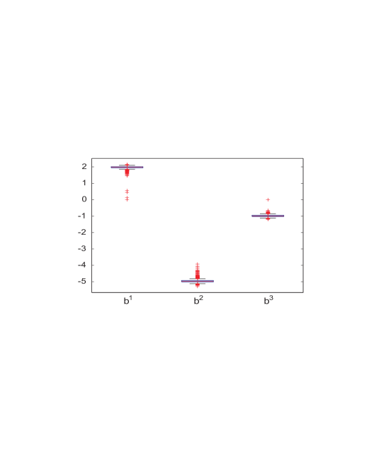
Figure 2: Box plot of the LS estimators for model $M_{1}$, $n$=30 (left); $n$=100 (right)

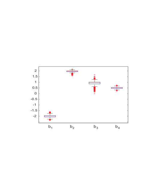
Figure 3: Box plot of the LS estimators for model $M_{2}$, $n$=30 (left); $n$=100 (right)

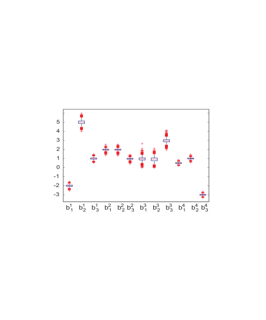
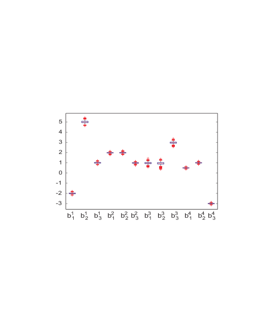
Figure 4: Box plot of the LS estimators for model $M_{3}$, $n$=30 (left); $n$=100 (right)

7 Conclusions

Previous linear regression models for interval data based on set arithmetic have been extended. In all cases the search of the LS estimators involves minimization problems with constraints. The constraints are necessary to assure the existence of the residuals and thus, the coherency of the estimated model with the population one.

A very flexible simple model based on the canonical decomposition and allowing for cross-relationships between mid-points and spreads has been introduced. An algorithm to find the exact LS-estimates has been developed. This model has been extended to the multiple case. The LS exact algorithm strongly relies on the geometry of the feasible set and it cannot be generalized in a simple way. However, the LS estimates can be found by applying the KKT conditions. The extension of the basic simple model in [9], which is not based on the canonical decomposition, requires a different approach, but the solutions can also be found by applying the KKT conditions.

The empirical validity of the estimation process for all the models has been shown by means of simulations. However, further theoretical studies of the main properties of the regression estimators, as the bias, the consistency or the asymptotic distributions should be pursued.

Table 1: Sample data for the daily blood pressures and the pulse rate ranges of $59$ patients

y	$\emph{{x}}_{1}$	$\emph{{x}}_{2}$	y	$\emph{{x}}_{1}$	$\emph{{x}}_{2}$	y	$\emph{{x}}_{1}$	$\emph{{x}}_{2}$
63-102	118-173	58-90	47-93	119-212	52-78	71-118	104-161	47-68
73-105	122-178	55-84	58-113	131-186	32-114	74-125	127-189	61-101
62-118	105-157	61-110	52-112	113-213	65-92	59-94	120-179	62-89
69-133	141-205	38-66	48-116	101-194	63-119	53-109	99-169	48-73
60-119	109-174	51-95	60-98	126-191	59-98	76-125	128-210	49-78
55-121	99-201	59-87	47-104	94-145	43-67	37-94	88-221	49-82
88-130	148-201	55-102	55-85	113-183	48-77	52-96	111-192	64-107
56-121	94-176	56-133	74-133	116-201	54-84	50-94	102-156	37-75
39-84	102-167	47-95	52-95	103-159	61-94	55-98	104-161	56-90
63-118	102-185	44-110	45-95	106-167	44-108	57-113	111-199	46-83
62-116	112-162	63-109	64-121	130-180	52-98	67-122	136-201	62-95
55-97	103-161	56-84	52-104	90-177	48-107	59-101	125-192	54-92
58-109	116-168	26-109	54-104	97-182	53-120	50-111	98-157	61-108
57-101	124-226	49-88	47-108	98-160	54-78	59-90	120-180	75-124
60-107	97-154	53-103	54-104	100-161	58-99	47-86	87-150	47-86
90-127	159-214	59-78	77-158	141-256	70-132	70-118	138-221	55-89
62-107	108-147	63-115	50-95	87-152	55-80	65-117	115-196	47-83
53-105	120-188	70-105	42-86	99-172	56-103	54-100	95-166	40-80
57-95	113-176	71-121	45-107	92-172	56-97	46-103	114-186	68-91
45-91	83-140	37-86	100-136	145-210	62-100

Table 2: Experimental results for the estimation of the linear models

Model	$\widehat{\nu}$ $\setminus$ $n$	$30$	$100$	$500$
		$\widehat{E}(\widehat{\nu})$  $\widehat{MSE}(\widehat{\nu})$	$\widehat{E}(\widehat{\nu})$  $\widehat{MSE}(\widehat{\nu})$	$\widehat{E}(\widehat{\nu})$  $\widehat{MSE}(\widehat{\nu})$
$M_{1}$	$\widehat{b_{1}}$	1.9732 0.0042	1.9858 0.0008	1.9933 0.0001
	$\widehat{b_{2}}$	-4.9627 0.0056	-4.9799 0.0013	-4.9909 0.0002
	$\widehat{b_{3}}$	-0.9809 0.0115	-0.9926 0.0070	-0.9961 0.0001
$M_{2}$	$\widehat{b^{1}}$	-2.0005 0.0097	-1.9997 0.0026	-2.0004 0.0005
	$\widehat{b^{2}}$	1.9651 0.0052	1.9809 0.0013	1.9911 0.0003
	$\widehat{b^{3}}$	0.9302 0.0230	0.9588 0.0060	0.9816 0.0011
	$\widehat{b^{4}}$	0.4991 0.0044	0.5004 0.0012	0.5000 0.0002
$M_{3}$	$\widehat{b_{1}^{1}}$	-2.0014 0.0114	-2.0004 0.0026	-2.0002 0.0005
	$\widehat{b_{2}^{1}}$	5.0017 0.0465	5.0007 0.0108	5.0001 0.0020
	$\widehat{b_{3}^{1}}$	1.0002 0.0111	1.0001 0.0027	1.0000 0.0005
	$\widehat{b_{1}^{2}}$	1.9738 0.0082	1.9837 0.0019	1.9920 0.0003
	$\widehat{b_{2}^{2}}$	1.9763 0.0100	1.9853 0.0020	1.9920 0.0004
	$\widehat{b_{3}^{2}}$	0.9722 0.0082	0.9841 0.0018	0.9918 0.0003
	$\widehat{b_{1}^{3}}$	0.9576 0.0413	0.9691 0.0090	0.9855 0.0015
	$\widehat{b_{2}^{3}}$	0.9097 0.0737	0.9429 0.0171	0.9717 0.0030
	$\widehat{b_{3}^{3}}$	2.9588 0.0410	2.9709 0.0087	2.9842 0.0015
	$\widehat{b_{1}^{4}}$	0.4996 0.0054	0.5003 0.0013	0.5001 0.0002
	$\widehat{b_{2}^{4}}$	0.9992 0.0060	1.0002 0.0014	1.0002 0.0003
	$\widehat{b_{3}^{4}}$	-2.9994 0.0053	-2.9995 0.0013	-3.0002 0.0003

List of Figure Captions

• Figure 1: $\Gamma_{G}$ for the sample data in Table 1

• Figure 2: Box plot of the LS estimators for Model $M_{1}$, $n=30$ (left); $n=100$ (right)

• Figure 3: Box plot of the LS estimators for Model $M_{2}$, $n=30$ (left); $n=100$ (right)

• Figure 4: Box plot of the LS estimators for Model $M_{3}$, $n=30$ (left); $n=100$ (right)

  Algorithm 1

     STEP 1: Compute the global minimum of $g$, $\widehat{\nu}=S_{2}^{-1}z_{2}$, with $z_{2}=(\widehat{\sigma}_{\emph{{x}}^{S},\emph{{y}}},\widehat{\sigma}_{\emph{{x}}^{C},\emph{{y}}})^{t}$ and $S_{2}$ the sample covariance matrix of $(\emph{{x}}^{S},\emph{{x}}^{C})$. If $\widehat{\nu}\in\Gamma_{G}$, then $\widehat{\nu}$ is the solution, else goto Step 2.

     STEP 2: Compute $r_{0}=\min_{i=1,\ldots,n}{\mathrm{spr}\emph{{y}}_{i}}/{|\mathrm{mid}\emph{{x}}_{i}|}$ and identify the straight line $l_{(v)}$ in the set $\{l_{k}:c=-u_{k}b+v_{k}\}_{k=1}^{n}$ such that $(0,r_{0})\in l_{(v)}$. If there exists more than one line in these conditions, then $l_{(v)}$ is the one for which the value $-\mathrm{spr}\emph{{y}}_{k}/|\mathrm{mid}\emph{{x}}_{k}|$ is lowest.

     STEP 3: Compute $s_{0}=\min_{i=1,\ldots,n}{\mathrm{spr}\emph{{y}}_{i}}/{\mathrm{spr}\emph{{x}}_{i}}$ and identify the straight line $l_{(h)}$ in the set $\{l_{k}:c=-u_{k}b+v_{k}\}_{k=1}^{n}$ such that $(s_{0},0)\in l_{(h)}$. If there exists more than one line in these conditions, then $l_{(h)}$ is the one for which the value $-\mathrm{spr}\emph{{y}}_{k}/|\mathrm{mid}\emph{{x}}_{k}|$ is greatest.

     bf STEP 4: Let $R=\{l_{(v)}\}$, $C=\{0,s_{0}\}$, $D=\{(v),(h)\}$, $j=1$ and $l_{(j)}=l_{(v)}$. If $(v)=(h)$, then redefine $R=\{l^{1}\},C=\{x^{0},x^{1}\}$, let $t=1$ and goto Step 8 else goto Step 5.

     STEP 5: Compute $(b_{(j,h)},c_{(j,h)})$ the intersection point of the lines $l_{(j)}$ and $l_{(h)}$. Check if $(b_{(j,h)},c_{(j,h)})\in\mathrm{fr}(\Gamma_{G})$, through the conditions

  • $b_{(j,h)}\in[0,s_{0}]$, and

  • $c_{(j,h)}=\min\{-u_{k}b_{(j,h)}+v_{k}:k=1,\ldots,n\}$.

  If $(b_{(j,h)},c_{(j,h)})\in\mathrm{fr}(\Gamma_{G})$, goto Step 7 else goto Step 6.

     STEP 6: Compute $(b_{(j,k)},c_{(j,k)})$ the intersection points of $l_{(j)}$ and each line in $\{l_{k}:c=-u_{k}b+v_{k}\}_{k=1}^{n}$ such that $k\notin D$. Take the line $l_{k^{*}}$ such that $(b_{(j,k^{*})},c_{(j,k^{*})})\in\mathrm{fr}(\Gamma_{G})$ (verifying the corresponding conditions i) and ii) shown in Step 5). If there exists more than one line in these conditions, choose as $l_{k^{*}}$ the one for which the value $-\mathrm{spr}\emph{{y}}_{k^{*}}/|\mathrm{mid}\emph{{x}}_{k^{*}}|$ is lowest. Let $R=R\cup\{l_{k*}\}$, $C=C\cup\{b_{(j,k*)}\}$, $D=D\cup\{k*\}$, $j=j+1$, $l_{(j)}=l_{k*}$, and goto Step 5.

     STEP 7: Let $R=R\cup\{l_{(h)}\}$ and $C=C\cup\{b_{(j,h)}\}$. Redefine $R=\{l_{(v)},l_{k^{*}_{1}},l_{k^{*}_{2}},\ldots,l_{k^{*}_{p}},l_{(h)}\}$ as $\{l^{1},l^{2},l^{3},\ldots,l^{t-1},l^{t}\}$, and $C=\{0,b_{(1,k^{*}_{1})},b_{(k^{*}_{1},k^{*}_{2})},\ldots,b_{(k^{*}_{p},h)},s_{0}\}$ as $\{x^{0},x^{1},x^{2},\ldots,x^{t-1},x^{t}\}$. Goto Step 8.

  
  

     STEP 8: For $i=1,\ldots,t$, compute the local minimum of $g$ over the segment corresponding to the line $l^{i}$ on $[x^{i-1},x^{i}]$, given by the analytic expressions

  $$\left\{\begin{array}[]{l}b_{*}^{i}=\max\big{\{}x^{i-1},\min\{b^{i},x^{i}\}\big{\}}\\ c_{*}^{i}=-u_{i}b_{*}^{i}+v_{i}\end{array}\right.$$

  where $\displaystyle b^{i}=\frac{u_{i}v_{i}\widehat{\sigma}_{\emph{{x}}^{C}}^{2}-v_{i}\widehat{\sigma}_{\emph{{x}}^{S},\emph{{x}}^{C}}-u_{i}\widehat{\sigma}_{\emph{{x}}^{C},\emph{{y}}}+\widehat{\sigma}_{\emph{{x}}^{S},\emph{{y}}}}{\widehat{\sigma}_{\emph{{x}}^{S}}^{2}+u_{i}^{2}\widehat{\sigma}_{\emph{{x}}^{C}}^{2}-2u_{i}\widehat{\sigma}_{\emph{{x}}^{S},\emph{{x}}^{C}}}.$ Compute $g(b_{*}^{i},c_{*}^{i})$. Take $(b_{L_{2}},c_{L_{2}})$ the point in $\{(b_{*}^{i},c_{*}^{i})\}_{i=1}^{t}$ for which the value $g(b_{*}^{i},c_{*}^{i})$ is lowest. Note that $(b_{L_{2}},c_{L_{2}})$ is the local minimum of $g$ over $L_{2}$.

     STEP 9: Compute $(b_{L_{1}},c_{L_{1}})$ the local minimum of $g$ over $L_{1}$, given by the analytic expressions

  $$\left\{\begin{array}[]{l}b_{L_{1}}=0\\ c_{L_{1}}=\max\Big{\{}0,\min\bigg{\{}\displaystyle\frac{\widehat{\sigma}_{\emph{{x}}^{C},\emph{{y}}}}{\widehat{\sigma}_{\emph{{x}}^{C}}^{2}},r_{0}\bigg{\}}\Big{\}}\end{array}\right.$$

  Compute $g(b_{L_{1}},c_{L_{1}})$.

     STEP 10: Compute $(b_{L_{3}},c_{L_{3}})$ the local minimum of $g$ over $L_{3}$, given by the analytic expressions

  $$\left\{\begin{array}[]{l}b_{L_{3}}=\max\Big{\{}0,\min\bigg{\{}\displaystyle\frac{\widehat{\sigma}_{\emph{{x}}^{S},\emph{{y}}}}{\widehat{\sigma}_{\emph{{x}}^{S}}^{2}},s_{0}\bigg{\}}\Big{\}}\\ c_{L_{3}}=0\end{array}\right.$$

  Compute $g(b_{L_{3}},c_{L_{3}})$.

     STEP 11: Take $(b^{*},c^{*})$ the point in $\{(b_{L_{j}},c_{L_{j}})\}_{j=1}^{3}$ whose value $g(b_{L_{j}},c_{L_{j}})$ is lowest. Note that $(b^{*},c^{*})$ is the local minimum of $g$ on $\mathrm{fr}(S_{G})$.

References

- [1] A. Beresteanu, and F. Molinari, Asymptotic properties for a class of partially identified models, Econometrica 76(4) (2008), pp. 763-814.
- [2] S. Yu, Q. Yu, G.Y.C. Wong, Consistency of the generalized MLE of a joint distribution function with multivariate interval-censored data, Journal of Multivariate Analysis 97 (2006) 720-732.
- [3] P. D’Urso, and P. Giordani, A robust fuzzy k-means clustering model for interval valued data, Computational Statistics 21(2) (2006), pp. 251-269.
- [4] P. Giordani, Three-way analysis of imprecise data, Journal of Multivariate Analysis 101 (2010), pp. 568-582.
- [5] E.M. Hashimoto, E.M. Ortega, V.G. Cancho, and G.M. Cordeiro On estimation and diagnostics analysis in log-generalized gamma regression model for interval-censored data, Statistics (2011).
- [6] S-K. Tse, C. Ding, and C. Yang, Optimal accelerated life tests under interval censoring with random removals: the case of Weibull failure distribution, Statistics 42(5) (2008), pp. 435-451.
- [7] P. Diamond, Least squares fitting of compact set-valued data, Journal of Mathematical Analysis and Applications 147 (1990), pp. 531-544.
- [8] M.A. Gil, A. Lubiano, M. Montenegro, and M.T. López-García, Least squares fitting of an affine function and strength of association for interval-valued data, Metrika 56 (2002), pp. 97-111.
- [9] G. González-Rodríguez, A. Blanco, N. Corral, and A. Colubi, Least squares estimation of linear regression models for convex compact random sets, Advances in Data Analysis and Classification 1 (2007), pp. 67-81.
- [10] G. González-Rodríguez, A. Colubi, and M. Montenegro, Testing linear independence in linear models with interval-valued data, Computational Statistics & Data Analysis 51 (2007), pp. 3002-3015.
- [11] A. Blanco-Fernández, N. Corral, and G. González-Rodríguez, Estimation of a flexible simple linear model for interval data based on set arithmetic, Computational Statistics and Data Analysis 55(9) (2011), pp. 2568-2578.
- [12] A. Blanco-Fernández, A. Colubi, and G. González-Rodríguez, Confidence sets in a linear regression model for interval data, Journal of Statistical Planning and Inference 142(6) (2012), pp. 1320-1329.
- [13] L. Billard, and E. Diday, Regression analysis for interval-valued data, Data Analysis, Classification and Related Methods, Proc. of 7th Conference IFCS, Kiers, H.A.L. et al. Eds. 1 (2000), pp. 369-374.
- [14] E.A. Lima Neto, and F.A.T. de Carvalho, Constrained linear regression models for symbolic interval-valued variables, Computational Statistics & Data Analysis 54 (2010), pp. 333-347.
- [15] C.F Manski, and E. Tamer, Inference on regressions with interval data on a regressor or outcome, Econometrica 70(2) (2002), pp. 519-546.
- [16] W. Trutschnig, G. González-Rodríguez, A. Colubi, and M.A Gil, A new family of metrics for compact, convex (fuzzy) sets based on a generalized concept of mid and spread, Information Sciences 179(23) (2009), pp. 3964-3972.
- [17] W. Näther, Linear statistical inference for random fuzzy data, Statistics 29(3) (1997), pp. 221-240.
- [18] R. Körner, R, On the variance of fuzzy random variables, Fuzzy Sets and Systems 92 (1997), pp. 83-93.