Stationary solutions of liquid two-layer thin film models

Abstract

We investigate stationary solutions of a thin-film model for liquid two-layer flows in an energetic formulation that is motivated by its gradient flow structure. The goal is to achieve a rigorous understanding of the contact-angle conditions for such two-layer systems. We pursue this by investigating a corresponding energy that favors the upper liquid to dewet from the lower liquid substrate, leaving behind a layer of thickness $h_{*}$. After proving existence of stationary solutions for the resulting system of thin-film equations we focus on the limit $h_{*}\to 0$ via matched asymptotic analysis. This yields a corresponding sharp-interface model and a matched asymptotic solution that includes logarithmic switch-back terms. We compare this with results obtained using $\Gamma$-convergence, where we establish existence and uniqueness of energetic minimizers in that limit.

1 Introduction

Understanding stability and dewetting behaviour of thin liquid films coating a solid or a liquid substrate is important in many technological applications and natural phenomena on the micro- to nano scale. They range from tear films of the human eye to organic photovoltaics to numerous applications in the polymer based semiconductor industry.

Typical film thicknesses for these applications may range from tens to hundreds of nanometers and, depending on the material composition, may be susceptable to rupture and formation of holes due to intermolecular forces. Such rupture processes typically initiate complex dewetting scenarios, where holes grow further and their trailing rims merge into polygonal networks which eventually decay into patterns of droplets, that evolve on a slow time scale towards a global minimal energy state.

The present study focusses on liquid substrates, that energetically favor an interface with the underlying solid. In this case the stages of the dewetting process for the upper liquid proceed to some extend in parallel to those exhibited during dewetting of a liquid film from a solid substrate. The latter system has been investigated much more intensely in recent decades, both, experimentally and theoretically. Examples of the complex pattern formation can be found in Sharma et al. [1] or Seemann et al. [2] and further experimental and theoretical investigations in numerous references in the recent reviews by Craster & Matar [3] and Herminghaus et al. [4].

For liquid-liquid dewetting, experimental studies depicting some of these dewetting stages have been conducted by various groups such as by Segalman & Green [5], Lambooy et al. [6], Slep et al. [7] or Wang et al. [8] for the standard system of liquid polystyrene (PS) on a liquid polymethylmethacrylate(PMMA) substrate. They include investigations of rupture and hole growth, dewetting dynamics and equilibrium contact angles the liquid droplets make with the underlying liquid layer, where now the contact line is fixed by two angle conditions instead of one, i.e. Youngs law is replaced by the Neumann triangle construction [9]. Following the pioneering study by Brochard-Wyart et al. [10], where various dewetting regimes are derived and analysed, stability of liquid-liquid systems were investigated by Danov et al. [11], Pototsky et al. [12], Golovin & Fisher [13]. Stationary states and the dynamics towards stationary states were studied by Pototsky et al. [14], by Craster & Matar [15] and by Bandyopadhyay & Sharma [16] and for the case of gravity-driven liquid droplets on a inclined liquid substrate by Kriegsmann & Miksis [17].

Interestingly, direct quantitative comparisons of theoretical with experimental results, in particular on micro- and nano-scale, regarding for example the morphology of the interfaces, as performed in Kostourou et al. [18], or equilibrium values of the Neumann triangle, as discussed in [7], still leave many issues in need to be explained, such as the dependency of the morphology of the interfaces on the rheology of the liquids, their layer thicknesses or material parameters. On the other side, even for the simplest mathematical models of Newtonian two-layer liquid systems, mathematical theory is still largely open and this is the main focus of the present study.

Here, we are guided by the many similarities to dewetting from a solid substrate, and expect that some of the mathematical analysis developed for liquid films dewetting from a solid substrate can be carried over to liquid substrates. In particular, we aim to extend the existing theory for liquid droplets on a solid substrate to the situation on a liquid substrate.

As a starting point we recall the work by Bertozzi et al. [19] regarding stationary states and coarsening of droplets on solid substrates, where they showed existence of smooth global solutions for positive data with bounded energy for the no-slip lubrication equation. In addition they prove existence of global minimizers and determine a family of positive periodic solutions for admissible intermolecular potentials consisting of long-range attractive and short range repulsive contribution, and investigate their linear stability. Further extensions were given in Laugesen & Pugh [20], where linear stability of stationary solutions for the thin film equation with Neumann boundary conditions or periodic boundary conditions was investigated. Extensions of the existence theory to thin film equations accounting for slip at the liquid-solid interface were given in Rump et al. [21] and Kitavtsev et al. [22]. Convergence to stationary solutions of the one-dimensional thin-film equation and the number of stationary states was recently investigated by Zhang [23].

The extension of the existence theory to two-layer liquid systems is given in Section 3, after the formulation of the problem. With the appropriate energy functional for the two-layer system of coupled thin-film equations for the interfacial heights $h_{1}$ and $h_{2}$ (see sketch in figure 1) together with Neumann boundary conditions, we show existence of smooth stationary solutions as well as existence of a global minimizer for the steady state problem.

Admissible intermolecular potentials for the liquid-liquid system are of the form

$$\phi(h_{2}-h_{1})=\frac{\phi_{*}}{\ell-n}\left[\ell\left(\frac{h_{*}}{h_{2}-h_{1}}\right)^{n}-n\left(\frac{h_{*}}{h_{2}-h_{1}}\right)^{\ell}\right],$$ (1.1)

where $h_{1}$ is the height of the liquid-liquid interface, $h_{2}$ the height of the free surface and its minimal value $\phi_{*}<0$ is attained at $h_{*}$. We note that such potentials are widely used in the literature, see e.g. the review [24]. A choice that is related to the standard Lennard-Jones potential and typically used in experiments is $(n,\ell)=(2,8)$, see e.g. [2].

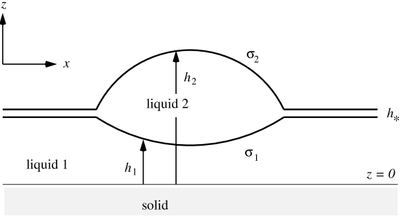
Fig. 1: Sketch of liquid droplet with surface tension $\sigma_{2}$ between air and liquid ₂ on top of a                   liquid layer with interfacial tension $\sigma_{1}$ between liquid ₂ and liquid ₁.

The Neumann triangle construction for contact angles at a triple junction is thereby replaced by properties of approximate contact angles resulting from the particular structure of the surface free energy $\phi$. Starting from this energetic formulation we seek to understand in Section 4 and 5 how the Neumann triangle construction is attained as a limit $h^{*}\to 0$. This in mind, we first derive in Section 4 a sharp-interface model in the limit of $h^{*}\to 0$ using matched asymptotic analysis. This yields the appropriate expression for the equilibrium contact angles of these droplet solutions and as a result the corresponding Neumann triangle.

We find that, while the equilibrium contact angle is easy to obtain, as expected, the complete asymptotic argument needs to include logarithmic switch-back terms. We note, in retrospect, since equilibrium droplet solutions for solid substrates can be considered as limiting cases for liquid lenses, similar terms should also appear in the matched asymptotic derivation for that problem.

Finally, in Section 5 we rigorously show existence and uniqueness of the limit $h_{*}\to 0$ within the framework of $\Gamma$-convergence. We obtain a sharp-interface problem for which we compute the Euler-Lagrange equations, from which one can immediately read off the contact angles. Existence and uniqueness of minimizers is shown here using a rearrangement inequality.

2 Formulation

We consider a layered system of two immiscible Newtonian liquids with negative spreading coefficient $\phi_{*}$. We assume the layered system lives in the two phases $\Omega_{1}$ and $\Omega_{2}$ defined by

$$\Omega_{1}(t) =\{(x,y,z)\in\mathbb{R}^{3}:0\leq z<{h_{1}}(t,x,y)\},$$ (2.1a)

$$\Omega_{2}(t) =\{(x,y,z)\in\mathbb{R}^{3}:{h_{1}}(t,x,y)\leq z<{h_{2}}(t,x,y)\},$$ (2.1b)

for all $t>0$ as sketched (in 2D) in figure 1. Typical applications use liquids such as PMMA for the liquid substrate $\Omega_{1}$ and PS as the upper liquid $\Omega_{2}$, both on a scale where gravity can be neglected and, for this study, unentangled and density matched. These simplifying assumptions allow us that the flow of the viscous and incompressible liquids in each phase $\Omega_{i}$ ($i=1,2$) is governed by the Stokes equation and the continuity equation:

$$-\nabla\cdot\bigl{(}-p_{i}\mathbb{I}+\mu_{i}(\nabla\mathbf{u}_{i}+\nabla\mathbf{u}_{i}^{\top})\bigr{)} =\mathbf{f}_{i},$$ (2.2a)

$$\nabla\cdot\mathbf{u}_{i} =0,$$ (2.2b)

together with a kinematic condition at each free boundaries $z=h_{i}$, i.e.

$$(\mathbf{e}_{z}\partial_{t}h_{i}-\mathbf{u}_{i})\cdot\mathbf{n}_{i}=0.$$ (2.3)

Here, $\mathbf{n}_{i}$ denotes the outer normal.

At the solid substrate a no-slip and an impermeability condition are imposed. At the liquid-liquid interface the velocity is continuous, i.e. $\mathbf{u}_{2}=\mathbf{u}_{1}$, and the tangential stress is continuous and the normal stress makes a jump proportional to the mean curvature $[[-p_{i}\mathbb{I}+\mu_{i}(\nabla\mathbf{u}_{i}+\nabla\mathbf{u}_{i}^{\top})]]_{1,2}\mathbf{n}_{1}=2\sigma_{1,2}\kappa\mathbf{n}_{1}$. The dewetting process is driven by the intermolecular potential of the upper liquid layer, i.e. $\mathbf{f}_{2}=-\nabla\phi$. We assume that the thickness of the lower layer is sufficiently thick, so other contributions to the intermolecular potential are negligible, i.e. $\mathbf{f}_{1}=0$.

In addition we assume that the the ratio $\varepsilon_{\ell}=H/L$ of the vertical to horizontal length scales is always small and the two-layer system can be approximated by a thin-film model. We denote by $L$ the length scale of the typical horizontal width and $H=h_{\rm max}$ the maximum of the difference $h_{2}-h_{1}$.

Detailed derivations of thin-film models for liquid-liquid systems are given for example in [17], [12] or recently, by accountung for interfacial slip, in [25]. For the convenience of the reader we note here the choice of non-dimensional variable and parameters, where the non-dimensional horizontal and vertical coordinates are given by $\tilde{x}=x/L$, $\tilde{y}=y/L$ and $\tilde{z}=z/h_{\rm max}$, respectively, and $\tilde{h}=h/h_{\rm max}$. The non-dimensional pressures $\tilde{p}_{i}=p_{i}/P$ and the derivative of the non-dimensional intermolecular potential $\phi^{\prime}_{\varepsilon}=\phi^{\prime}/P$ are scaled such that $P=\phi_{*}n\ell/\bigl{(}(\ell-n)h_{\rm max}\bigr{)}$ and hence

$${\phi_{\varepsilon}}^{\prime}(\tilde{h})=\frac{1}{\varepsilon}\left[\left(\frac{\varepsilon}{\tilde{h}}\right)^{n+1}-\left(\frac{\varepsilon}{\tilde{h}}\right)^{\ell+1}\right]$$ (2.4)

attains the minimal value $\min{\phi_{\varepsilon}}=-1$ at $\tilde{h}=\varepsilon$, where $\varepsilon=h_{*}/h_{\rm max}$ is the non-dimensional thickness of the ultra-thin film. For the dynamic problem, the velocities are scaled with the characteristic horizontal velocity of the dewetting upper layer, such that for the non-dimensional horizontal and vertical velocities we have $\tilde{u}=u/U$, $\tilde{v}=v/U$ and $\tilde{w}=w/\varepsilon_{\ell}U$, respectively, with $U=\varepsilon_{\ell}^{3}\sigma_{2}/\mu_{2}$, and the non-dimensional time $\tilde{t}=(U/L)t$.

For the remainder of this paper it is convenient to introduce the ratios $\sigma=\sigma_{1}/\sigma_{2}$ and $\mu=\mu_{1}/\mu_{2}$ of surface tensions and viscosities, respectively, and drop all the “$\sim$”. Within this approximation the normal and tangential stress conditions at the free surface $h_{2}$ and at the free liquid-liquid interface $h_{1}$ yield the expressions for the pressures $p_{2}$ and $p_{1}$

$$p_{1}=-\sigma\Delta h_{1}-\displaystyle{\phi^{\prime}_{\varepsilon}}(h_{2}-h_{1}),\quad\qquad p_{2}=-\Delta h_{2}+{\phi^{\prime}_{\varepsilon}}(h_{2}-h_{1}),$$ (2.5)

respectively. Under these assumptions the coupled system of nonlinear fourth order partial differential equations for the profiles of the free surfaces $h_{1}$ and $h_{2}$ takes the form

$$\partial_{t}{\bf h} =\nabla\cdot\left({Q}\cdot\nabla{\bf p}\right),$$ (2.6)

where ${\bf h}=(h_{1},h_{2})^{\top}$ is the vector of liquid-liquid interface profile and liquid-air surface profile. The components of the vector ${\bf p}=(p_{1},p_{2})^{\top}$ are the interfacial pressures given in (2.5). The gradient of the pressure vector is multiplied by the mobility matrix $Q$ which is given by

$${Q}=\frac{1}{\mu}\left[\begin{array}[]{cccc}\displaystyle\frac{h_{1}^{3}}{3}&\;\displaystyle\frac{h_{1}^{3}}{3}+\frac{h_{1}^{2}(h_{2}-h_{1})}{2}\\ \\ \displaystyle\frac{h_{1}^{3}}{3}+\frac{h_{1}^{2}(h_{2}-h_{1})}{2}&\quad\;\displaystyle\frac{\mu}{3}(h_{2}-h_{1})^{3}+h_{1}h_{2}(h_{2}-h_{1})+\frac{h_{1}^{3}}{3}\end{array}\right].$$ (2.10)

We proceed to first show existence of stationary solution to the system (2.4)-(2.10) with Neumann and Dirichlet boundary conditions on a finite domain $\Omega=(0,L)\subset\mathbb{R}$.

3 Energy functionals and existence of stationary solutions

Consider the two-layer thin film equations (2.5)-(2.10) defined on $\Omega=(0,L)\subset\mathbb{R}$ with
Neumann boundary conditions:

$$\partial_{x}h_{1}=\partial_{x}h_{2}=\partial_{xxx}h_{1}=\partial_{xxx}h_{2}=0\ \ \text{for}\ \ x\in\partial\Omega.$$ (3.1)

The energy functional associated to the gradient flow of the lubrication equation is given by

$$E_{\varepsilon}(h_{1},h_{2})=\int_{0}^{L}\left[\frac{\sigma}{2}\left|\partial_{x}h_{1}\right|^{2}+\frac{1}{2}\left|\partial_{x}h_{2}\right|^{2}+{\phi_{\varepsilon}}(h_{2}-h_{1})\right]dx$$ (3.2)

where the potential function ${\phi_{\varepsilon}}$ is given as in (2.4) with $(n,\ell)=(2,8)$. The relation to the thin-film equations is $p_{i}=\delta E_{\varepsilon}/\delta h_{i}$. From (2.5)-(2.10) and (3.1) conservation of mass follows

$$\int_{\Omega}h_{1}(t,x)\,dx =m_{1},$$ (3.3a)

$$\int_{\Omega}\left(h_{2}(t,x)-h_{1}(t,x)\right)\,dx =m_{2}\ \ \text{for all}\ \ t>0,$$ (3.3b)

where $m_{1}$ and $m_{2}$ are positive constants. Any stationary solution of (2.5)-(2.10) with (3.1) satisfies

$$0=Q\cdot\partial_{x}{\bf p}$$ (3.4)

in $\Omega$, where the mobility matrix $Q$ is not singular i.e. ${\rm det}Q\neq 0$ for all $h_{1},\,{h_{2}-h_{1}}>0$. Therefore, one obtains that any positive stationary solution of (2.5)-(2.10) satisfies $\partial_{x}p_{1}=\partial_{x}p_{2}=0$ in $\Omega$. This in turn is equivalent to

$$\sigma\partial_{xx}h_{1} =-\phi_{\epsilon}^{\prime}(h_{2}-h_{1})-\lambda_{2}+\lambda_{1},$$ (3.5a)

$$\partial_{xx}h_{2} =\phi_{\epsilon}^{\prime}(h_{2}-h_{1})-\lambda_{1},$$ (3.5b)

where constants $\lambda_{2}$ and $\lambda_{1}$ are Lagrange multipliers associated with conservation of mass (3.3a) and (3.3b), respectively. To solve (3.5) let us consider the equation for the difference

$$h(t,x)=h_{2}(t,x)-h_{1}(t,x)$$

which reads as follows

$$\partial_{xx}h=\frac{\sigma+1}{\sigma}\phi_{\epsilon}^{\prime}(h)+\frac{1}{\sigma}\lambda_{2}-\frac{\sigma+1}{\sigma}\lambda_{1}.$$ (3.6)

For brevity we set

$$P:=-\frac{1}{\sigma}\lambda_{2}+\frac{\sigma+1}{\sigma}\lambda_{1}.$$

According to [19] for positive $P$, there exists a so called droplet solution $\bar{h}$ to (3.6) satisfying boundary conditions (3.1), such that $\bar{h}(y+L/2)$ is an even function and monotone decreasing for $y\in(0,L/2)$.

For this solution the asymptotics and main properties are derived in the next section, here we consider $\bar{h}$ as a known analytical function and integrate (3.5) two times w.r.t. $x$. We then obtain a solution to (3.5) with (3.1) in the form

$$h_{1}=-\frac{1}{\sigma+1}\bar{h}-\frac{1}{2}\frac{\lambda_{2}}{\sigma+1}x^{2}+Cx+C_{1},$$

$$h_{2}=\frac{\sigma}{\sigma+1}\bar{h}-\frac{1}{2}\frac{\lambda_{2}}{\sigma+1}x^{2}+Cx+C_{1}.$$ (3.7)

Using now again (3.1) one obtains that $\lambda_{2}=0,\ C=0$ and

$$h_{1}=-\frac{1}{\sigma+1}\bar{h}+C_{1},$$

$$h_{2}=\frac{\sigma}{\sigma+1}\bar{h}+C_{1}.$$ (3.8)

The additive constant $C_{1}$ and the remaining Lagrange multiplier are determined from the conservation of masses (3.3a) and (3.3b), respectively. We conclude that the solution (3.8) is given by combination of two symmetric droplets with constant outer layer. The next theorem establishes existence of a global minimizer to the energy functional (3.2) and shows that it satisfies (3.5) with (3.1).

Theorem 1.

Let $\Omega$ be a bounded domain of class $C^{0,1}$ in $\mathbb{R}\,^{d},\,d\geq 1$ and let $\mathbf{m}=(m_{1},m_{2})$ with $m_{1},m_{2}>0$. Then a global minimizer of $E_{\epsilon}(\cdot,\cdot)$ defined in (3.2) exists in the class

$$X_{\mathbf{m}}:=\left\{(h_{1},h_{2})\in H^{1}(\Omega)^{2}:m_{1}=\int_{\Omega}h_{1},\ m_{2}=\int_{\Omega}(h_{2}-h_{1}),\ h_{2}\geq h_{1}\right\},$$ (3.9)

For $d=1$ and $\Omega=(0,\,L)$ the function ${h_{2}-h_{1}}$ is strictly positive and $(h_{1},h_{2})$ are smooth solutions to the ODE system (3.5) with (3.1) and

$$\lambda_{1}=\frac{1}{L}\int_{\Omega}\phi_{\epsilon}^{\prime}(h_{2}-h_{1})\,dx,\quad\lambda_{2}=0.$$ (3.10)

Proof.

Even though the proof proceeds very analogously to the one of Theorem 2-3 in [19] using direct methods of the calculus of variations, for the convenience of the reader we give here for our system.

Let $(h_{1}^{k},h_{2}^{k})_{k\in\mathrm{N}}$ be a minimizing sequence which exists since $E_{\epsilon}(m_{1},m_{2}+m_{1})<\infty$. Observe that $\phi_{\epsilon}(\cdot)$ is bounded from below by a constant. Hence, a constant $C_{2}$ exists such that

$$\int_{\Omega}|\partial_{x}h_{1}^{k}|^{2}+|\partial_{x}h_{2}^{k}|^{2}\,dx\leq C_{2}\ \text{for all}\ k\in\mathrm{N}.$$ (3.11)

Rellich’s compactness theorem implies that a subsequence (again denoted by $(h_{1}^{k},h_{2}^{k})_{k\in\mathrm{N}})$ exists which converges strongly in $L^{2}(\Omega)^{2}$ and pointwise almost everywhere to $(h_{1},h_{2})\in H^{1}(\Omega)^{2}$. By Fatou’s lemma, we deduce that also $\phi_{\epsilon}(h_{2}-h_{1})$ lies in $L^{1}(\Omega)$. Using the weak lower semicontinuity of the norm, we obtain

$$E_{\epsilon}(h_{1},h_{2})\leq\lim\inf_{k\rightarrow\infty}E_{\epsilon}(h_{1}^{k},h_{2}^{k})=\inf_{(\bar{h}_{1},\bar{h}_{2})\in V}E_{\epsilon}(\bar{h}_{1},\bar{h}_{2}).$$

Consequently, $(h_{1},h_{2})$ is a minimizer and the integrability of $\phi_{\epsilon}(h_{2}-h_{1})$ implies that $h_{2}-h_{1}>0$ almost everywhere in $\Omega$.

Let now $d=1$ and $\Omega=(0,\,L)$. The estimate (3.11) implies

$$\int_{\Omega}|\partial_{x}(h_{2}^{k}-h_{1}^{k})|^{2}\,dx\leq C_{3}.$$

Next, the boundedness of $\int\phi_{\epsilon}(h_{2}^{k}-h_{1}^{k})\,dx$ and definition of $\phi_{\epsilon}$ imply a uniform in $k$ bound on $||(h_{2}^{k}-h_{1}^{k})^{-4}||_{2}$. Using this, one can estimate

$$\int_{0}^{L}|\partial_{x}((h_{2}^{k}-h_{1}^{k})^{-3})|\,dx =3\int_{0}^{L}\frac{|\partial_{x}(h_{2}^{k}-h_{1}^{k})|}{(h_{2}^{k}-h_{1}^{k})^{4}}\,dx$$

$$\leq 3||\partial_{x}(h_{2}^{k}-h_{1}^{k})||_{2}\ ||(h_{2}^{k}-h_{1}^{k})^{-4}||_{2}\leq C_{4},$$

where $C_{4}$ is constant. Owing to the continuous embedding of $W^{1,3}(0,1)$ into $L^{\infty}(0,1)$ the strong positivity of $h_{2}-h_{1}$ follows. This in turn implies the differentiability of the function $F_{\epsilon}(s):=E_{\epsilon}(h_{1}+s\varphi_{1},h_{2}+s\varphi_{2})$ considered with fixed $(\varphi_{1},\varphi_{2})\in H^{1}(0,L)^{2}$ for sufficiently small $s$. Since $(h_{1},h_{2})$ is a minimizer, by differentiation of $F_{\epsilon}(s)$ at $s=0$, we obtain that

$$\int_{0}^{L}(-\sigma\partial_{xx}h_{1}-\phi_{\epsilon}^{\prime}(h_{2}-h_{1}))\varphi_{1}+(-\partial_{xx}h_{2}+\phi_{\epsilon}^{\prime}(h_{2}-h_{1}))\varphi_{2}\,dx=0,$$

for all $(\varphi_{1},\varphi_{2})\in H^{1}(0,L)^{2}$ such that

$$\int_{0}^{L}\varphi_{1}\,dx=\int_{0}^{L}(\varphi_{2}-\varphi_{1})\,dx=0.$$

Without this constraint, using Lagrangian multipliers and testing with general $(\psi_{1},\psi_{2})\in H^{1}(0,L)^{2}$ this yields

$$\int_{0}^{L}\Big{[}(-\sigma\partial_{xx}h_{1}-\partial_{xx}h_{2})\psi_{1}+(-\partial_{xx}h_{2}+\phi_{\epsilon}^{\prime})\psi_{2}\Big{]}dx-\frac{1}{L}\int_{0}^{L}\int_{0}^{L}\phi_{\epsilon}^{\prime}\,dy\,\psi_{2}\,dx=0.$$

Standard elliptic regularity theory then implies that $(h_{1},h_{2})$ are smooth solutions to (3.5) together with (3.1) and (3.10). ∎

Remark 2.

Note, that for Dirichlet boundary conditions we can proceed as follows: Let us impose on system (3.5) the Dirichlet boundary conditions

$$h_{1}(0)=h_{1}(L)=A,\ \ h_{2}(0)=h_{2}(L)=B,$$ (3.12)

such that

$$B-A=\min_{x\in(0,L)}\bar{h}(x),$$ (3.13)

where $\bar{h}$ is the Neumann solution to (3.6) defined above. In this case it follows again that $h_{2}-h_{1}=\bar{h}$. Consequently, $h_{1}$ and $h_{2}$ are given by (3.7) with constants $\lambda_{1},\lambda_{2},C,C_{1}$ determined uniquely by (3.12) and conservation of mass (3.3a)-(3.3b). Using (3.13) and the asymptotics for $\bar{h}$ one obtains that the leading order of the solution (3.7) as $\varepsilon\rightarrow 0$ has now the form

$$h_{1}(x) =\frac{1}{2}\frac{\lambda_{1}-\lambda_{2}}{\sigma}\left((x-\tfrac{L}{2})^{2}-s^{2}\right)+C_{1},\ \ x\in\omega$$

$$h_{2}(x) =-\frac{1}{2}\lambda_{1}\left((x-\tfrac{L}{2})^{2}-s^{2}\right)+C_{1},\ \ x\in\omega$$

$$h_{1}(x) =h_{2}(x)=-\frac{1}{2}\frac{\lambda_{2}}{\sigma+1}\left((x-\tfrac{L}{2})^{2}-s^{2}\right)+C_{1},\ \ x\in(0,L)\setminus\omega,$$ (3.14)

where $\omega=(L/2-s,L/2+s)$ and

$$s^{2}=\frac{2\sigma(\sigma+1)}{\left(\lambda_{2}-(\sigma+1)\lambda_{1}\right)^{2}}.$$

In contrast to the solution of (3.14) with Neumann conditions, solutions with Dirichlet boundary conditions are not constant but quadratic in the ultra-thin layer $(0,L)\setminus\omega$.

4 Matched asymptotic solution and contact angles

Note first that the system of equations for $h_{1}$ and $h_{2}$ (3.4) is equivalent to following system for $h_{1}$ and $h$

$$0 =\partial_{x}\left(-\sigma\partial_{xx}h_{1}-\phi_{\varepsilon}^{\prime}(h)\right),$$ (4.1a)

$$0 =\partial_{x}\left(-\frac{\sigma}{\sigma+1}\partial_{xx}h+\phi^{\prime}_{\varepsilon}(h)\right).$$ (4.1b)

where we denote $\sigma=\sigma_{1}/\sigma_{2}$, see [25] for a more detailed derivation. For our asymptotic analysis, this is convenient, since now for the variable $h=h_{2}-h_{1}$ we can distinguish the core droplet region, which we will call the “outer region” and the adjacent thin regions of thickness $\varepsilon$, which we call the “inner region”. We will derive a sharp-interface limit using matched asymptotic analysis in the limit as $\varepsilon\to 0$. For this we first write the equations in the form such that the intermolecular potential is small in the core region and becomes order one in the adjacent thin regions. Using $(n,\ell)=(2,8)$ we define

$$\phi^{\prime}_{\varepsilon}(h)=\displaystyle\frac{1}{\varepsilon}\Phi^{\prime}\left(\displaystyle\frac{h}{\varepsilon}\right)$$ (4.2)

4.1 Stationary solution for $\boldsymbol{h}$

As we will later show rigorously, we can assume that the droplet is (axi)symmetric and the profile a decreasing function, so that without loss of generality, the maximum of $h$ is at the origin of our coordinate system. Now consider the problem $h$ and $x\geq 0$

$$0=\partial_{x}\left[\frac{\sigma}{\sigma+1}\partial_{xx}h-\frac{1}{\varepsilon}\Phi^{\prime}\left(\displaystyle\frac{h}{\varepsilon}\right)\right],$$ (4.3a)

$$\lim_{x\to\infty}h=h_{\infty},\quad\lim_{x\to\infty}\partial_{x}h=0,\quad\lim_{x\to\infty}\partial_{xx}h=0.$$ (4.3b)

We can integrate this twice and use the conditions as $x\to\infty$ to fix the integration constants to obtain

$$\partial_{x}h=\sqrt{2\frac{\sigma+1}{\sigma}}\sqrt{\Phi\left(\frac{h}{\varepsilon}\right)-\Phi\left(\frac{h_{\infty}}{\varepsilon}\right)-\frac{1}{\varepsilon}\Phi^{\prime}\left(\frac{h_{\infty}}{\varepsilon}\right)\left(h-h_{\infty}\right)}$$ (4.4)

The solution to this problem shows a steep decline in height towards $O(\varepsilon)$ in an $\varepsilon$-strip around $x=s$, where we would like to determine the apparent contact-angle. This can be obtained by writing the problem in so-called outer and inner coordinates, valid in the core and the adjacent thin regions, and matching as $\varepsilon\to 0$. Interestingly, while it is easy to obtain the condition for the contact angle, it turns out that in order to carry out the complete matching consistently, we need to go up to second order in the matching, in order to account for the logarithmic switch-back terms, that come into play in this problem, see [26] for a discussion of these terms.

Note, that the coefficient $(\sigma+1)/\sigma$ can be removed by rescaling $x$ appropriately, leading to the classical problem of a droplet of height $h$ on a solid substrate. Interestingly, to our knowledge for this problem the above mentioned logarithmic switch-back terms have not been noticed before.

Outer problem

The symmetry of the problem leads us to the condition that at the symmetry axis $x=0$ we have

$$\partial_{x}h=0$$ (4.5)

It is also convenient to normalize the height such that $h(0)=1$. In this case we obtain from (4.4) an algebraic equation for $h_{\infty}$ and $\varepsilon$ that can be approximated as $\varepsilon\to 0$.

$$0=\Phi\left(\frac{1}{\varepsilon}\right)-\Phi\left(\frac{h_{\infty}}{\varepsilon}\right)-\frac{1}{\varepsilon}\Phi^{\prime}\left(\frac{h_{\infty}}{\varepsilon}\right)\left(1-h_{\infty}\right)$$ (4.6)

Solving this by making the ansatz for the asymptotic expansion for $h_{\infty}$

$$h_{\infty}=\varepsilon h_{\infty,0}+\varepsilon^{2}h_{\infty,1}+\varepsilon^{3}h_{\infty,2}+O(\varepsilon^{4})$$ (4.7)

we obtain

$$h_{\infty,0}=1,\quad h_{\infty,1}=\frac{1}{16},\quad h_{\infty,2}=\frac{45}{512},\quad$$ (4.8)

Next, we assume that the asymptotic solution to the outer problem can be represented by the expansion

$$h(x;\varepsilon)=f_{0}(x)+\varepsilon f_{1}(x)+\varepsilon^{2}f_{2}(x)+O(\varepsilon^{3}).$$ (4.9)

The leading order outer problem then becomes

$$\partial_{x}f_{0}=-\sqrt{\frac{3}{4}\frac{\sigma+1}{\sigma}\left(1-f_{0}\right)},$$ (4.10a)

$$f_{0}(0)=1$$ (4.10b)

which has the solution

$$f_{0}(x)=-\frac{3}{16}\frac{\sigma+1}{\sigma}x^{2}+1.$$ (4.11)

Hence, the leading order outer solution will vanish as $x$ approaches the location

$$s=\frac{4}{\sqrt{3}}\sqrt{\frac{\sigma}{\sigma+1}}$$ (4.12)

However, the full solution does not vanish and will be obtained by matching to the solution of the “inner” problem near $s$. We will find that in order to complete the solution, we will need to solve the expansion up-to second order. We find for $f_{1}$ and $f_{2}$

$$\partial_{x}f_{1}=\frac{f_{1}}{x}-\frac{3}{16}\frac{\sigma+1}{\sigma}\,x,$$ (4.13a)

$$f_{1}(0)=0$$ (4.13b)

and

$$\partial_{x}f_{2}=2\frac{f_{2}}{x}+\frac{1}{x}\left(\frac{8}{3}\frac{1}{f_{0}^{2}}+\frac{1}{16}\left(f_{0}-1\right)-\frac{2}{3}\left(f_{0}+3\right)+2f_{1}\right)+\frac{3}{8}\frac{\sigma+1}{\sigma}\,x$$ (4.14a)

$$f_{2}(0)=0$$ (4.14b)

Inner problem

The solution of the inner problem lives in an $\varepsilon$ neighborhood of $x=s$ and extends towards $x\to+\infty$. It will be matched to the outer problem in the other direction. Hence we introduce the inner variables $v(z)$ and independent variable $z$ via

$$h(x)=\varepsilon\,v(z;\varepsilon)\quad\mbox{and}\quad x=s+\varepsilon z.$$ (4.15)

Rewriting the problem (4.4) in these coordinates and making the ansatz

$$v(z;\varepsilon)=v_{0}(z)+\varepsilon v_{1}(z)+O(\varepsilon^{2})$$ (4.16)

we find to leading order the problem

$$\partial_{z}v_{0}=-\sqrt{2\frac{\sigma+1}{\sigma}}\sqrt{-\frac{1}{2v_{0}^{2}}+\frac{1}{8v_{0}^{8}}+\frac{3}{4}}$$ (4.17)

and to $O(\varepsilon)$ the problem

$$\partial_{z}v_{1}=-\sqrt{2\frac{\sigma+1}{\sigma}}\sqrt{-\frac{1}{2v_{0}^{2}}+\frac{1}{8v_{0}^{8}}+\frac{3}{4}}\,\,\frac{{3}v_{0}^{9}(v_{0}-1)+8v_{1}(1-v_{0}^{6})}{2v_{0}(4v_{0}^{6}-3v_{0}^{8}-1)}$$ (4.18)

We solve and match in the inner coordinates and obtain by expanding $v$ at $z=-\infty$

$$v_{0}+\varepsilon v_{1} = -\frac{\sqrt{3}}{2}\sqrt{\frac{\sigma+1}{\sigma}}\,z+a_{1}-\frac{4}{9}\sqrt{3\frac{\sigma}{\sigma+1}}\,\frac{1}{z}+\cdots$$ (4.19)

$$+\varepsilon\left(-\frac{3}{16}\frac{\sigma+1}{\sigma}\,z^{2}+\frac{\sqrt{3}}{4}\frac{\sigma+1}{\sigma}(a_{1}-1)\,z-\ln(-z)\right.$$

$$\hskip 56.9055pt\left.+C+\frac{1}{6}+\frac{2}{3}\sqrt{3\frac{\sigma}{\sigma+1}}(a_{1}+1)\frac{1}{z}+\cdots\right).$$

For the corresponding outer expansion we have

$$\frac{f_{0}+\varepsilon f_{1}+\varepsilon^{2}f_{2}}{\varepsilon} = -\frac{\sqrt{3}}{2}\sqrt{\frac{\sigma+1}{\sigma}}\,z-1-\frac{4}{9}\sqrt{3\frac{\sigma}{\sigma+1}}\,\frac{1}{z}+\cdots$$ (4.20)

$$+\varepsilon\left(-\frac{3}{16}\frac{\sigma+1}{\sigma}\,z^{2}-\frac{\sqrt{3}}{2}\frac{\sigma+1}{\sigma}\,z-\ln(-z)\right.$$

$$\hskip 28.45274pt\left.-\ln\left(\frac{\sqrt{3}}{8}\sqrt{\frac{\sigma+1}{\sigma}}\right)-\frac{19}{96}-\ln(\varepsilon)+\cdots\right).$$

We note that all of the terms in the first row of (4.19) and (4.20) match provided $a_{1}=-1$. The terms in the second row match provided

$$C=-\ln(\varepsilon)-\frac{35}{96}-\ln\left(\frac{\sqrt{3}}{8}\sqrt{\frac{\sigma+1}{\sigma}}\right)$$ (4.21)

where we note the appearance of a so-called “logarithmic switch-back” term $\ln(\varepsilon)$. Hence, the composite solution is

$$\bar{h} = \varepsilon\left[v_{0}\left(\frac{x-s}{\varepsilon}\right)+\frac{\sqrt{3}}{2}\sqrt{\frac{\sigma+1}{\sigma}}\,\frac{x-s}{\varepsilon}\right]$$

$$+\varepsilon^{2}\left[v_{1}\left(\frac{x-s}{\varepsilon}\right)+\frac{3}{16}\frac{\sigma}{\sigma+1}\left(\frac{x-s}{\varepsilon}\right)^{2}+\frac{\sqrt{3}}{2}\frac{\sigma+1}{\sigma}\,\frac{x-s}{\varepsilon}\right]$$

$$+f_{0}(x)+\varepsilon\Big{[}f_{1}(x)+1\Big{]}$$

$$+\varepsilon^{2}\left[f_{2}(x)+\frac{4}{9}\sqrt{\frac{3\sigma}{\sigma+1}}\,\frac{1}{x-s}+\ln\left(s-x\right)+\frac{19}{96}+\ln\left(\frac{\sqrt{3}}{8}\sqrt{\frac{\sigma+1}{\sigma}}\right)\right]$$

with $s$ given in equation (4.12) and for $x<s$. For $x\geq s$ only the inner expansion $\bar{h}=\varepsilon v_{0}+\varepsilon^{2}v_{1}$ remains.

Fig. 2: Top: Comparison of the composite solution $h_{c}$ (dashed curve) with the numerical solution of (4.3) (solid curve), for $\varepsilon=0.2$ and $\sigma=1.2$. Bottom: Solutions for $h_{1}$ and $h_{2}$ reconstructed from the composite solution $\bar{h}$ for $\sigma=1.2$ and $\varepsilon=0.05$ (dashed curve) and $\varepsilon=0.2$ (dotted curve) and the solution to the sharp interface model (4.25) (solid curve).

Stationary solution for $h_{1}$ and $h_{2}$

To complete the solution, we determine the solution to the liquid-liquid interface $h_{1}$ simply by adding equations (4.1a) and (4.1b). Then we integrate thrice and use the far-field conditions $\partial_{xx}h,\partial_{x}h,\partial_{xx}h_{1},\partial_{x}h_{1}\to 0$, $h\to h_{\infty}$ and $h_{1}\to d$ as $x\to\pm\infty$ to fix the constants. This results in $h_{1}$ being

$$h_{1}=-\frac{1}{\sigma+1}\left(h-h_{\infty}\right)+d,$$ (4.23)

and equivalently $h_{2}$ is

$$h_{2}=\frac{\sigma}{\sigma+1}\left(h-h_{\infty}\right)+d+h_{\infty}.$$ (4.24)

Here $d$ denotes the height $h_{1}$ as $x\to\pm\infty$ and we assume $d$ to be large enough so that $h_{1}$ never becomes negative. Also note that for other boundary conditions, such as e.g. Dirichlet conditions mentioned in the previous section, further contributions will arise. Unlike the solutions for droplets on solid substrates, here new families of profiles for the ultra-thin film connecting a droplet to the boundaries or to other droplets arise.

In figure 2 we compare our asymptotic solution with the numerical solution. Observe that the $O(\varepsilon)$ solution already gives an excellent approximation of the exact solution for $\varepsilon=0.2$, where the exact solution is approximated by the higher-order numerical solution of the boundary value problem. This suggests that a sharp-interface model should also be a good approximation of the full model. The sharp-interface model for $h$ is simply the leading order outer problem for $h$, but now with boundary conditions, that result from the leading order matching. Hence, we obtain

$$0=\partial_{xxx}f_{0}$$ (4.25a)

with boundary conditions

$$f_{0}=0\quad\mbox{and}\quad\partial_{x}f_{0}=\partial_{z}v_{0}=-\sqrt{-2\frac{\sigma+1}{\sigma}\Phi(1)}\quad\mbox{at}\quad x=\pm s$$ (4.25b)

where the contact angle has been determined via matching. Equivalently, for the half-droplet, by imposing symmetry we have the boundary conditions

$$f_{0}(s)=0,\quad\partial_{x}f_{0}(s)=-\sqrt{-2\frac{\sigma+1}{\sigma}\Phi(1)}\quad\mbox{and}\quad\partial_{x}f_{0}(0)=0$$ (4.26)

In the following section we show how the sharp-interface model is obtained via $\Gamma$-convergence and also proof existence and uniqueness of its solutions.

5 Sharp-interface limit via $\boldsymbol{\Gamma}$-convergence

In this section we investigate properties of stationary solutions of the sharp-interface two-layer model. Such model can be obtained by considering the limiting problem $\varepsilon\to 0$ in the framework of $\Gamma$-convergence. For one-layer systems corresponding minimizers are known as mesoscopic droplets [21]. In this approach equilibrium contact angles can be directly deduced from the Euler-Lagrange equation of the resulting $\Gamma$-limit energy. On the other hand showing an equi-coerciveness property we have that the sequence of minimizers of $E_{\varepsilon}$ converges to a minimizer of the $\Gamma$-limit energy $E_{\infty}$.

For boundary conditions $h_{1}=h_{2}$ and certain domains we show that solutions of the minimization problem $\min_{(h_{1},h_{2})}E_{\infty}$ exist and are unique up-to translations. The main technique used here is the symmetric-rearrangement, see e.g. [27, 28].

For the section to come we consider energies such as in (3.2). For later convenience we define ${W_{\varepsilon}}(h)=\bigl{(}{\phi_{\varepsilon}}(h)-\Phi(1)\bigr{)}/|\Phi(1)|$ where as before $W(h)={W_{\varepsilon}}(h/\varepsilon)$ is independent of $\varepsilon$. The shift by $|\Phi(1)|$ has the advantage of working with a non-negative energy without changing the Euler-Lagrange equations.

With these definitions consider the following family of minimization problems. For $\Omega\subset\mathbb{R}^{n}$ bounded with Lipschitz boundary and $m_{1},m_{2}>0$ given and $\varepsilon>0$ we look for minimizers of $E_{\varepsilon}:X_{\mathbf{m}}\to\mathbb{R}^{\infty}$ defined as

$$E_{\varepsilon}(h_{1},h_{2})=\int_{\Omega}\frac{\sigma}{2}|\nabla h_{1}|^{2}+\frac{1}{2}|\nabla h_{2}|^{2}+\,|\Phi(1)|\,{W_{\varepsilon}}(h_{2}-h_{1})$$ (5.1)

with $\sigma>0$ and ${W_{\varepsilon}}(h)=W\bigl{(}h/\varepsilon\bigr{)}$ as $\varepsilon\to 0$. Note that nonnegativity $h_{1}>0$ is not enforced because otherwise extra terms in $E_{\varepsilon}$ are required.

5.1 $\boldsymbol{\Gamma}$-convergence

For a given domain $\Omega\subset\mathbb{R}^{n}$ bounded with Lipschitz boundary define the space of admissible interfaces as before in (3.9) by

$$X_{\mathbf{m}}:=\left\{(h_{1},h_{2})\in H^{1}(\Omega)^{2}:m_{1}=\int_{\Omega}h_{1},\ m_{2}=\int_{\Omega}(h_{2}-h_{1}),\ h_{2}\geq h_{1}\right\},$$ (5.2)

and in general let $W:\mathbb{R}\to\mathbb{R}$ be a function with the properties

1. $W\geq 0$  and  $W(h)=0\Leftrightarrow h=1$.

2. $W(h)\xrightarrow{h\to+\infty}1$ and $W(h)\leq 1$ for $h>1$.
   

We want to investigate the family of minimization problems (5.1). First we note that the sequence $E_{\varepsilon}$ is equi-coercive in the weak topology of $H^{1}(\Omega)^{2}$. This is a simple consequence of

$$E_{\varepsilon}(h_{1},h_{2})\geq c(\|\nabla h_{1}\|_{H^{1}}^{2}+\|\nabla h_{2}\|_{H^{1}}^{2}),$$

which holds for all $(h_{1},h_{2})\in X_{\mathbf{m}}$. Together with the $\Gamma$-convergence the equi-coercivity implies the following abstract convergence result. We know that any sequence $\{h_{1,n},h_{2,n}\}$ of minimizers to the energies $E_{\varepsilon_{n}}$ has a weakly converging subsequence $(h_{1,n},h_{2,n})\rightharpoonup(h_{1}^{*},h_{2}^{*})$. Furthermore the limit $(h_{1}^{*},h_{2}^{*})$ is a minimizer of the $\Gamma$-limit energy $E_{\infty}$. This relates minimizers of $E_{\varepsilon}$ to minimizers of the $\Gamma$-limit $E_{\infty}$.

Now we investigate the $\Gamma$-limit of (5.1) in the topology of weak convergence in the space $H^{1}(\Omega)^{2}$. We recall the definition of $\Gamma$-convergence , see also [29, 30].

Definition 3.

We say that a sequence $E_{\varepsilon}:X\to\mathbb{R}^{\infty}$ $\Gamma$-converges in $X$ in the weak topology to $E_{\infty}:X\to\mathbb{R}^{\infty}$ if for all $x\in X$ we have

• (lim-inf inequality) For every sequence $\{x_{\varepsilon}\}\subset X$ weakly converging to $x$ there holds

  $$E_{\infty}(x)\leq\liminf_{\varepsilon}E_{\varepsilon}(x_{\varepsilon}).$$

• (lim-sup inequality) There exists a sequence $\{x_{\varepsilon}\}\subset X$ weakly converging to $x$ such that

  $$E_{\infty}(x)\geq\limsup_{\varepsilon}E_{\varepsilon}(x_{\varepsilon}).$$

The function $E_{\infty}$ is called the $\Gamma$-limit of $(E_{\varepsilon})$, and we write $E_{\infty}\!=\!\Gamma\text{-}\lim_{\varepsilon}E_{\varepsilon}.$

The key proposition to compute the overall $\Gamma$-limit is to consider the $\Gamma$-limit of the potential separately. Here we use that weak convergence in $H^{1}$ implies strong convergence in $L^{2}$ and the right continuity of $q\mapsto\int\chi\{h>q\}$ for any given $h\in H^{1}$.

Proposition 4.

Consider the functional $F_{\varepsilon}:H^{1}(\Omega)\to\mathbb{R}^{\infty}$ defined as

$$F_{\varepsilon}(h)=\begin{cases}\int_{\Omega}{W_{\varepsilon}}(h)&h\in X_{m},\\ \infty&\text{otherwise},\end{cases}$$

where

$$X_{m}=\left\{h\in H^{1}(\Omega):h\geq 0,\int_{\Omega}h=m\right\}.$$

Then

$$\Gamma\text{-}\lim_{\varepsilon}F_{\varepsilon}(h)=F_{\infty}(h)=\begin{cases}\int_{\Omega}\chi\{h>0\}&h\in X_{m},\\ \infty&\text{otherwise},\end{cases}$$

with $\chi$ being the characteristic function.

Proof.

Consider an arbitrary sequence $\varepsilon_{n}\to 0$ and $h\in X_{m}$.
(i) (lim-inf condition)
Let $\{h_{n}\}\subset X_{m}$ such that $h_{n}\rightharpoonup h$ weakly in $H^{1}(\Omega)$, then $h_{n}\to h$ strongly in $L^{2}(\Omega)$. Choose $\delta_{n}\to 0$ such that ${\varepsilon_{n}/\delta_{n}}\to 0$ as $n\to\infty$ which immediately gives

$$\liminf_{n}\int_{\Omega}W_{\varepsilon_{n}}(h_{n}) \geq\liminf_{n}\int_{\{h_{n}>\delta_{n}\}}W_{\varepsilon_{n}}(h_{n})\,\,{=}\,\,\liminf_{n}\int_{\Omega}\chi\{h_{n}>\delta_{n}\}.$$ (5.3)

Next we want to use $\int\chi\{h>0\}\leq\liminf\int_{\Omega}\chi\{h_{n}>\delta_{n}\}$. Conversely assume

$$\liminf_{n}\int_{\Omega}\chi\{h_{n}>\delta_{n}\}<\int\chi\{h>0\}.$$ (5.4)

Then employing right-continuity of $s\mapsto\int_{\Omega}\chi\{h>s\}$ (see [27], Proposition 6.1) there must exist some $\delta,\bar{\delta}>0$ such that

$$0 <\liminf_{n}\int_{\Omega}\chi\{h>0\}-\chi\{h_{n}>\delta_{n}\}-\delta\leq\liminf_{n}\int_{\Omega}\chi\{h>\bar{\delta}\}-\chi\{h_{n}>\delta_{n}\},$$

$$\leq\liminf_{n}\int_{\Omega}\chi\{h>\bar{\delta}\mathrm{\,\,\&\,\,}h_{n}<\delta_{n}\}\leq\left(\frac{2}{\bar{\delta}}\right)^{2}\liminf_{n}\int_{\Omega}|h-h_{n}|^{2}=0,$$

where we used Chebyshev’s inequality. This is a contradiction and thus by the previous assertions

$$\liminf_{n}\int_{\Omega}W_{\varepsilon_{n}}(h_{n})\geq\int_{\Omega}\chi\{h>0\}.$$

(ii) (lim-sup condition)
Define a recovery sequence by $h_{n}=\alpha_{n}h+\varepsilon_{n}$ where $\alpha_{n}={(m-\varepsilon_{n}|\Omega|)}/{m}$. Then $h_{n}\in X_{m}$ and $h_{n}\to h$ even strongly in $H^{1}(\Omega)$ and the following estimate holds

$$\limsup_{n}\int_{\Omega}{W_{\varepsilon}}_{n}(h_{n}) =\limsup_{n}\Big{(}\int_{\{h>0\}}W\left(1+\frac{\alpha_{n}}{\varepsilon_{n}}h\right)+\int_{\{h=0\}}W\left(1+\frac{\alpha_{n}}{\varepsilon_{n}}h\right)\Big{)}\,,$$

$$\leq\limsup_{n}\int_{\Omega}\chi\{h>0\}+\int_{\{h=0\}}W\left(1\right)=\int_{\Omega}\chi\{h>0\}\,,$$

where we used that $W(s)\leq 1$ for $s>1$ and $W(1)=0$. ∎

To prove the $\Gamma$-convergence to the sharp-interface model we can exploit the property that the behavior of gradient terms can be easily controlled.

Theorem 5.

For the family of energies (5.1) the $\Gamma$-limit is

$$E_{\infty}(h_{1},h_{2})=\int_{\Omega}\frac{\sigma}{2}|\nabla h_{1}|^{2}+\frac{1}{2}|\nabla h_{2}|^{2}+|\Phi(1)|\,\chi\{h_{2}>h_{1}\}$$

Proof.

The gradient terms in $E_{\varepsilon}$ are weakly lower semicontinuous with respect to weak convergence in $H^{1}(\Omega)^{2}$. Together with Proposition 4 this gives the lim-inf inequality. On the other hand the gradient terms are continuous with respect to strong convergence in $H^{1}(\Omega)^{2}$. Choosing the recovery sequence as in the proof of Proposition 4 one gets the desired lim-sup inequality. ∎

Now we want to deduce necessary conditions for minimizers of $E_{\infty}$. We are especially interested in conditions at the points where the two-phase domain meets the one-phase domain. One problem is that one cannot immediately compute the Euler-Lagrange equations ($L^{2}$-gradient) of the sharp-interface energy functional $E_{\infty}$. This is due to $\int_{\Omega}\chi\{h_{2}>h_{1}\}$ being only lower semicontinuous in the strong $H^{1}(\Omega)$ topology, but not continuous nor differentiable. In fact directional derivatives of this part of the energy will almost surely be zero or infinite. Therefore we compute the directional derivative of $E_{\infty}$ in another topology as follows: For ease of notation introduce

$$\omega=\{x\in\Omega:h_{2}>h_{1}\}$$ (5.5)

and restrictions of $h_{1}$ and $h_{2}$ to $\omega$ and $\Omega\setminus\omega$ are called

$$h_{1}:=h_{1}|_{\omega},\quad h_{2}:=h_{2}|_{\omega},\quad h:=h_{1}|_{\Omega\setminus\omega}=h_{2}|_{\Omega\setminus\omega},$$

with boundary condition $h_{1}=h_{2}=h$ on $\partial\omega$. We will now vary $h_{1},h_{2}$ and $h$ but also $\omega$. The formal calculation is restricted to smooth $h_{1},h_{2},h$ and $\omega$. Using these we can rewrite the energy using the restrictions as

$$E_{\infty}(h_{1},h_{2},h,\omega) =\int_{\omega}\left[\frac{\sigma}{2}|\nabla h_{1}|^{2}+\frac{1}{2}|\nabla h_{2}|^{2}+|\Phi(1)|\right]+\int_{\Omega\setminus\omega}\frac{\sigma^{\prime}}{2}|\nabla h|^{2},$$ (5.6)

where we define $\sigma^{\prime}:=1+\sigma$. A perturbation of $\tau\mapsto\bigl{(}h_{1}(\tau),h_{2}(\tau),h(\tau),\omega(\tau)\bigr{)}$ can be parametrised using a diffeomorphism $\psi(\circ,\tau):\Omega\to\Omega$ with the property that $\omega(\tau)=\{\psi(x,\tau):x\in\omega(0)\}$. In the same spirit define $\bar{h}_{1}(x_{0},\tau)=h_{1}(\psi(x_{0},\tau),\tau)$ as the pullback of $h_{1}$ by $\psi$ and similarly $\bar{h}_{2}$ and $\bar{h}$. The boundary conditions $\partial_{\tau}{\bar{h}_{1}}=\partial_{\tau}{\bar{h}_{2}}=\partial_{\tau}{\bar{h}}$ on $\partial\omega(\tau)$ translate into

$$\dot{h}_{1}+\dot{\psi}\cdot\nabla h_{1}=\dot{h}_{2}+\dot{\psi}\cdot\nabla h_{2}=\dot{h}+\dot{\psi}\cdot\nabla h=:\dot{\xi}.$$ (5.7)

Here we use the notation $\dot{\psi}:=\partial_{\tau}\psi$, $\dot{h}_{1}:=\partial_{\tau}h_{1}$, $\dot{h}_{2}:=\partial_{\tau}h_{2}$ and $\dot{h}:=\partial_{\tau}h$. Then using Reynolds transport theorem we get

$$\frac{d}{d\tau}E_{\infty}(h_{1},h_{2},h,\omega)= \int_{\omega}\left({\sigma}\nabla h_{1}\nabla\dot{h}_{1}+\nabla h_{2}\nabla\dot{h}_{2}\right)+\int_{\Omega\setminus\omega}{\sigma^{\prime}}\nabla h\nabla\dot{h}$$

$$\quad+\int_{\partial\omega}\left[\frac{\sigma}{2}|\nabla h_{1}|^{2}+\frac{1}{2}|\nabla h_{2}|^{2}-\frac{\sigma^{\prime}}{2}|\nabla h|^{2}+|\Phi(1)|\right](n\cdot\dot{\psi}).$$

Applying integration-by-parts and boundary conditions (5.7) yields in one and two spatial dimensions, i.e. $\omega\subset\mathbb{R}$ and $\omega\subset\mathbb{R}^{2}$ the directional derivative

$$0= \frac{d}{d\tau}\Big{(}E_{\infty}+\lambda_{2}\int h_{1}+\lambda_{1}\int(h_{2}-h_{1})\Big{)},$$

$$= -\int_{\omega}\bigl{[}\sigma\Delta h_{1}+\lambda_{2}-\lambda_{1}\bigr{]}\dot{h}_{1}+\bigl{[}\Delta h_{2}+\lambda_{1}\bigr{]}\dot{h}_{2}\,\,-\int_{\Omega\setminus\omega}\bigl{[}\sigma^{\prime}\Delta h+\lambda_{2}\bigr{]}\dot{h}$$

$$\,\,+\int_{\partial\omega}\left[-\frac{\sigma}{2}(\nabla h_{1})^{2}-\frac{1}{2}(\nabla h_{2})^{2}+\frac{\sigma^{\prime}}{2}(\nabla h)^{2}+|\Phi(1)|+\eta^{2}\bigl{(}1+\sigma-\sigma^{\prime}\bigr{)}\right](n\cdot\dot{\psi})$$

$$\,\,+\int_{\partial\omega}\left[\sigma(n\cdot\nabla h_{1})+(n\cdot\nabla h_{2})-\sigma^{\prime}(n\cdot\nabla h)\right]\bigl{(}\dot{\xi}+(t\cdot\dot{\psi})\bigr{)}.$$ (5.8)

where $\eta^{2}:=(t\cdot\nabla h_{1})^{2}\equiv(t\cdot\nabla h_{2})^{2}\equiv(t\cdot\nabla h)^{2}$. The expressions inside square brackets have to vanish independently, since the perturbations $(\dot{h}_{1},\dot{h}_{2},\dot{h},\dot{\xi},\dot{\psi})$ are independent.

Remark 6.

Above we added Lagrange multipliers $\lambda_{1},\lambda_{2}$ to take care of the mass conservation. In one dimension there is no tangential contribution and hence $\eta\equiv 0$, whereas in two dimensions the contribution with $\eta^{2}$ vanishes due to definition $\sigma^{\prime}=\sigma+1$. However, if $\sigma^{\prime}$ could be choosen independently of $\sigma$, there would be an extra contribution in that case.

5.2 Existence and uniqueness of solutions

In this part we consider the sharp interface energy derived by $\Gamma$-convergence and study its minimizers. The idea of the proof is to show that for a minimizer the support of

$$h:=h_{2}-h_{1}$$ (5.9)

is a ball contained in $\Omega$, on which the solutions can be computed explicitly. The minimization itself is performed with masses $\mathbf{m}=(m_{1},m_{2})$ held fixed. Further extensions of our proof and properties of the solutions are discussed in the end of this section.

Definition 7.

Let $A\subset\mathbb{R}^{n}$ a Borel set of finite Lebesgue measure, then the symmetric rearrangement of the set $A$ is defined by $A^{*}=\mathcal{B}_{s}(0)$ with $s$ such that $\mu(A)=\mu(A^{*})$. The symmetric decreasing rearrangement of the characteristic function is $(\chi_{A})^{*}=\chi_{A^{*}}$. Now let $f:\mathbb{R}^{n}\to\mathbb{R}$ a Borel measureable function vanishing at infinity, then define the symmetric-decreasing rearrangement of $f$ by

$$f^{*}(x)=\int_{0}^{\infty}\chi^{*}_{\{f>s\}}(x)\,{\rm d}s.$$

Theorem 8.

(Minimizer of sharp interface energy) Let $\Omega=\mathcal{B}_{R}(0)$ and $X=\{(h_{1},h_{2})\in X_{\mathbf{m}}(\Omega):(h_{1}-h_{2})|_{\partial\Omega}=0\}$ and energy

$$E(h_{1},h_{2}) :=\int_{{\Omega}}\frac{\sigma}{2}|\nabla h_{1}|^{2}+\frac{1}{2}|\nabla h_{2}|^{2}\ +|\Phi(1)|\,\chi_{\{h_{2}>h_{1}\}}\ {\rm d}x.$$ (5.10)

Then using $\zeta(x):=\alpha(s^{2}-|x|^{2})^{+}$ minimizers of $E$ with mass $(m_{1},m_{2})$ are

$$h_{2}=\frac{\sigma}{\sigma+1}\zeta(x-x_{0})+h,\qquad h_{1}(x)=h_{2}-\zeta(x-x_{0}),$$ (5.11)

with constant $x_{0}\in\Omega$ and $r,\alpha,h\in\mathbb{R}$. Prescribing the mass $(m_{1},m_{2})$ fixes $r$ and $h$, whereas $\alpha$ is fixed by the contact angle (Neumann triangle)

$${\sigma}(\nabla h_{1})^{2}+{}(\nabla h_{2})^{2}=2|\Phi(1)|,\qquad\text{ at }|x|=r.$$ (5.12)

For large masses $m_{2}$ (5.12) is not required and we get $r=R$, $x_{0}=0$ in (5.11).

Proof.

Using similar ideas as in [21], we proceed as follows:

Symmetry: For given $(h_{1},h_{2})\in X$ let $h=(h_{2}-h_{1})\in H^{1}_{0}({\Omega})$ as in (5.9), non-negative let

$$\lambda:=\frac{\|\nabla h_{2}\|}{\|\nabla h\|}\geq 0.$$

Using Cauchy-Schwarz inequality in $L^{2}(\Omega)$ the following energy estimate holds

$$E(h_{1},h_{2}) \geq(\sigma+1)\|\nabla h_{2}\|^{2}+\sigma\|\nabla h\|^{2}-2\sigma\|\nabla h_{2}\|\ \|\nabla h\|+|\Phi(1)|\mu(\{h>0\}),$$

$$=\|\nabla h\|^{2}\left(\lambda^{2}+\sigma(1-\lambda)^{2}\right)+|\Phi(1)|\mu(\{h>0\}).$$

Minimizing with respect to $\lambda$ gives the lower bound

$$E(h_{1},h_{2}) \geq\frac{\sigma}{\sigma+1}\|\nabla h\|^{2}+|\Phi(1)|\mu(\{h>0\})$$

which is attained only if $\lambda={\sigma}/{(\sigma+1)}$ and $\nabla h_{2}$ is a multiple of $\nabla h$. Now let $h^{*}$ be the symmetric-decreasing rearrangement of $h$, then by virtue of the Pólya-Szegő inequality

$$\int_{\mathbb{R}^{n}}h^{*}\ {\rm d}x=\int_{\mathbb{R}^{n}}h\ {\rm d}x,\qquad\qquad\|\nabla h^{*}\|_{L^{2}(\mathbb{R}^{n})}\leq\|\nabla h\|_{L^{2}(\mathbb{R}^{n})}.$$

We have the freedom to translate $h^{*}$ as long its support is contained in $\Omega$. Equality holds only if $h$ is already symmetric-decreasing [28]. Now assume that $h$ is not symmetric decreasing, or $\nabla h\neq\sigma/(\sigma+1)\nabla h_{2}$. Then we can reduce the energy by defining $h^{*}_{1}$ and $h^{*}_{2}$ by

$$h^{*}_{2}(x) :=\frac{\sigma}{\sigma+1}h^{*}(x-x_{0})+h,\qquad h^{*}_{1}(x):=h^{*}_{2}(x)-{h^{*}}(x-x_{0}),$$

and have $\nabla h^{*}_{2}=\lambda\nabla h^{*}$ and $\mu\{h>0\}=\mu\{h^{*}>0\}$ so that

$$E(h_{1},h_{2})>\frac{\sigma}{\sigma+1}\|\nabla{h^{*}}\|^{2}+|\Phi(1)|\mu(\{{h^{*}}>0\})=E(h^{*}_{1},h^{*}_{2}).$$

Note that by definition $\{h^{*}>0\}=\mathcal{B}_{s}(0)=:\omega^{*}$ with $s$ such that $\mu(\omega^{*})=\mu(h>0)$. To check $\zeta(x)=\alpha(s^{2}-|x|^{2})^{+}$ is now analogous to [21]. One has to solve the Euler-Lagrange equation for the first variation of $E$ given in (5.8) using standard methods. ∎

Corollary 9.

Let $X$ be as before and the sharp interface energy

$$E_{\infty}(h_{1},h_{2},h,\omega) :=\int_{\omega}\left(\frac{\sigma}{2}|\nabla h_{1}|^{2}+\frac{1}{2}|\nabla h_{2}|^{2}\ +|\Phi(1)|\right)\!\!\ {\rm d}x+\int_{\Omega\setminus\omega}\frac{\sigma^{\prime}}{2}|\nabla h|^{2}\ {\rm d}x$$ (5.13)

as in (5.6) for $\sigma^{\prime}>0$ arbitrary. Then the minimizers of (5.10) and (5.13) in $X$ are identical.

Proof.

Since we have $h=0$ on $\partial\omega$ the estimates of the previous proof are valid if the domain of integration is restricted to $\omega$. By construction we have $\|\nabla h\|_{L^{2}(\Omega\setminus\omega)}^{2}\geq\|\nabla h^{*}\|_{L^{2}(\Omega\setminus\omega^{*})}^{2}=0$. ∎

Remark 10.

Using the abbreviation $c=|\Phi(1)|(\sigma+1)/\sigma$ we can easily compute the parameters $r$ and $\alpha$ from the previous theorem and get

$$s_{1d} =\left(\frac{9m_{2}^{2}}{8c}\right)^{1/4}\!\!\!,\quad \alpha_{1d} =\left(\frac{2c^{3}}{9m_{2}^{2}}\right)^{1/4}\!\!\!,$$

$$s_{2d} =\left(\frac{8m_{2}^{2}}{\pi^{2}c}\right)^{1/6}\!\!\!,\qquad \alpha_{2d} =\left(\frac{\pi c^{2}}{2m_{2}}\right)^{1/3}\!\!\!.$$

in one and two spatial dimension respectively. The contact angles are then

$$\mathbf{n}\cdot\left.\nabla h_{1}\right|_{s_{-}}=\pm\frac{\sqrt{2c}}{1+\sigma} \mathbf{n}\cdot\left.\nabla h_{2}\right|_{s_{-}}=\mp\sqrt{2c}\frac{\sigma}{1+\sigma}.$$ (5.14)

and which actually holds in any spatial dimension. We also have

$$\mathbf{n}\cdot\nabla(h_{2}-h_{1})=\sqrt{2c}=\sqrt{-\frac{2(\sigma+1)}{\sigma}\Phi(1)}$$ (5.15)

which can be compared with the appropriate boundary condition in (4.25) from the matched asymptotic expansion.

Discussion and Outlook

We considered stationary solutions of systems of coupled thin-film equations for two-layer liquid films. After proving existence of stationary droplet solutions, we used matched asymptotic analysis to derive a corresponding sharp-interface model in the limit when the thickness of the ultra-thin film in the dewetted region $\varepsilon\to 0$, which then yields the equilibrium Neumann angles. We point out that our asymptotic analysis requires the inclusion of logarithmic switch-back terms for the asymptotic droplet solution, which should in principle also be needed for the limiting case of droplet solutions on solid substrates.

We then proved the existence and uniqueness of the sharp-interface model using the variational structure of the equations allowing us to formulate the problem as a minimization problem, for which we can study the limit $\varepsilon\to 0$ via $\Gamma$-convergence. In one spatial dimension on an interval both sharp-interface models are equivalent. In particular the contact angle of $h$ from the matched asymptotic analysis in (4.25) is the same as the one from the $\Gamma$-convergence in (5.15). Since the recovery of $h_{1},h_{2}$ from $h$ in both cases works via (4.23, 4.24) or (5.11), the second contact angle agrees as well. We note that dimensions $d>1$ one has to prove that the shape of the domain $\{h_{2}-h_{1}>0\}$ is a ball of a certain radius. Using symmetric decreasing rearrangement this property, and thereby existence and uniqueness of minimizers, could be proved.

We expect that, as for thin films on solid substrate, the techniques of matched asymptotic analysis can be extended to the dynamic time-dependent problem. In particular, the derivation and study of the time-dependent sharp-interface model will also support the understanding of the energetic structure of the system of the coupled thin film model and should still be valid in the time-dependent problem, e.g. in the gradient flow structure of a sharp-interface model. This will be important in the study of dewetting regimes, dewetting rates and the stability properties of the evolving interfaces, as it was done previously for the dewetting liquid films from solid substrates, see e.g. [31, 32].

As pointed out in the beginning of our study, mathematical theory for two-layer liquid flows leaves still many open questions and problems to be addressed. The present work can only be considered as a first step. Moreover, even considering only stationary solutions, we note that the general picture is much richer compared to the situation on a solid substrate, with energy structures leading to phase-inverted or more complicated patterns, and is be subject of our ongoing research.

References

• Sharma and Reiter [1996] A. Sharma and G. Reiter. Instability of thin polymer films on coated substrates: Rupture, dewetting and drop formation. J. Colloid Interface Sci., 178:383–389, 1996.
• Seemann et al. [2001] R. Seemann, S. Herminghaus, and K. Jacobs. Gaining control of pattern formation of dewetting films. Journal of Physics: Condensed Matter, 13:4925–4938, 2001.
• Craster and Matar [2009] R. V. Craster and O. K. Matar. Dynamics and stability of thin liquid films. Rev. Mod. Phys., 81:1131–1198, 2009.
• Herminghaus et al. [2008] S. Herminghaus, M. Brinkmann, and R. Seemann. Wetting and dewetting of complex surface geometries. Annual Review of Materials Research, 38:101–121, 2008.
• Segalman and Green [1999] R.A. Segalman and P.F. Green. Dynamics of rims and the onset of spinodal dewetting at liquid/liquid interfaces. Macromolecules, 32(3):801–807, 1999.
• Lambooy et al. [1996] P. Lambooy, K.C. Phelan, O. Haugg, and G. Krausch. Dewetting at the liquid-liquid interface. Physical review letters, 76(7):1110–1113, 1996.
• Slep et al. [2000] D. Slep, J. Asselta, M. H. Rafailovich, J. Sokolov, D. A. Winesett, A. P. Smith, H. Ade, and S. Anders. Effect of an Interactive Surface on the Equilibrium Contact Angles in Bilayer Polymer Films. Langmuir, 16:2369–2375, 2000.
• Wang et al. [2001] C. Wang, G. Krausch, and M. Geoghegan. Dewetting at a Polymer- Polymer Interface: Film Thickness Dependence. Langmuir, 17(20):6269–6274, 2001.
• Neumann [1894] F.E. Neumann. Vorlesung über die Theorie der Capillarität. BG Teubner: Leipzig, pages 113–116, 1894.
• Brochard-Wyart et al. [1993] F. Brochard-Wyart, P. Martin, and C. Redon. Liquid/liquid dewetting. Langmuir, 9(12):3682–3690, 1993.
• Danov et al. [1998] K.D. Danov, V.N. Paunov, N. Alleborn, H. Raszillier, and F. Durst. Stability of evaporating two-layered liquid film in the presence of surfactant–i. the equations of lubrication approximation. Chemical engineering science, 53(15):2809–2822, 1998.
• Pototsky et al. [2004] A. Pototsky, M. Bestehorn, D. Merkt, and U. Thiele. Alternative pathways of dewetting for a thin liquid two-layer film. Phys. Rev. E, 70(2):025201, Aug 2004.
• Fisher and Golovin [2005] L.S. Fisher and A.A. Golovin. Nonlinear stability analysis of a two-layer thin liquid film: Dewetting and autophobic behavior. Journal of colloid and interface science, 291(2):515–528, 2005.
• Pototsky et al. [2005] A. Pototsky, M. Bestehorn, D. Merkt, and U. Thiele. Morphology changes in the evolution of liquid two-layer films. The Journal of chemical physics, 122:224711, 2005.
• Craster and Matar [2006] R.V. Craster and O.K. Matar. On the dynamics of liquid lenses. Journal of colloid and interface science, 303(2):503–516, 2006.
• Bandyopadhyay and Sharma [2006] D. Bandyopadhyay and A. Sharma. Nonlinear instabilities and pathways of rupture in thin liquid bilayers. The Journal of chemical physics, 125:054711, 2006.
• Kriegsmann and Miksis [2003] J.J. Kriegsmann and M.J. Miksis. Steady motion of a drop along a liquid interface. SIAM Journal on Applied Mathematics, pages 18–40, 2003.
• Kostourou et al. [2010] K. Kostourou, D. Peschka, A. Münch, B. Wagner, S. Herminghaus, and R. Seemann. Interface morphologies in liquid/liquid dewetting. Chemical Engineering and Processing: Process Intensification, 2010.
• Bertozzi et al. [2001] A.L. Bertozzi, G. Grün, and T.P. Witelski. Dewetting films: bifurcations and concentrations. Nonlinearity, 14:1569–1592, 2001.
• Laugesen and Pugh [2000] RS Laugesen and MC Pugh. Linear stability of steady states for thin film and Cahn-Hilliard type equations. Archive for Rational Mechanics and Analysis, 154(1):3–51, 2000.
• Otto et al. [2007] F. Otto, T. Rump, and D. Slepčev. Coarsening rates for a droplet model: Rigorous upper bounds. SIAM Journal on Mathematical Analysis, 38(2):503–529, 2007.
• Kitavtsev et al. [2010] G. Kitavtsev, L. Recke, and B. Wagner. Asymptotics for the spectrum of a thin film equation in a singular limit. WIAS preprint, 2010.
• Zhang [2009] Y. Zhang. Counting the stationary states and the convergence to equilibrium for the 1-D thin film equation. Nonlinear Analysis, 71(5-6):1425–1437, 2009.
• Oron et al. [1997] A. Oron, S. H. Davis, and S. G. Bankoff. Long-scale evolution of thin liquid films. Rev. Mod. Phys., 69(3):931–980, 1997.
• Jachalski et al. [2011] S. Jachalski, A. Münch, D. Peschka, and B. Wagner. Thin film models for two-layer flows with interfacial slip. WIAS Preprint Number, 2011.
• Lagerstrom [1988] P. A. Lagerstrom. Matched Asymptotic Expansions: Ideas and Techniques. Springer Verlag, 1988.
• Leoni [2009] G. Leoni. A first course in Sobolev spaces. American Mathematical Society, 2009. ISBN 0821847686.
• Lieb and Loss [2001] E.H. Lieb and M. Loss. Analysis, volume 14. American Mathematical Society, 2001. ISBN 0821827839.
• Braides [2002] A. Braides. Gamma-convergence for Beginners. Oxford University Press, 2002. ISBN 0198507844.
• Dal Maso [1993] G. Dal Maso. Introduction to Gamma-convergence. Birkhäuser, 1993. ISBN 081763679X.
• Münch et al. [2006] A. Münch, B. Wagner, and T. P. Witelski. Lubrication models with small to large slip lengths. J. Engr. Math., 53:359–383, 2006.
• King et al. [2008] J. R. King, A. Münch, and B. Wagner. Linear stability analysis of a sharp-interface model for dewetting thin films. J. Engrg. Math., 63:177–195, 2008.