An absolutely stable discontinuous Galerkin method for the indefinite time-harmonic Maxwell equations with large wave number

Abstract

This paper develops and analyzes an interior penalty discontinuous Galerkin (IPDG) method using piecewise linear polynomials for the indefinite time harmonic Maxwell equations with the impedance boundary condition in the three dimensional space. The main novelties of the proposed IPDG method include the following: first, the method penalizes not only the jumps of the tangential component of the electric field across the element faces but also the jumps of the tangential component of its vorticity field; second, the penalty parameters are taken as complex numbers of negative imaginary parts. For the differential problem, we prove that the sesquilinear form associated with the Maxwell problem satisfies a generalized weak stability (i.e., inf-sup condition) for star-shaped domains. Such a generalized weak stability readily infers wave-number explicit a priori estimates for the solution of the Maxwell problem, which plays an important role in the error analysis for the IPDG method. For the proposed IPDG method, we show that the discrete sesquilinear form satisfies a coercivity for all positive mesh size $h$ and wave number $k$ and for general domains including non-star-shaped ones. In turn, the coercivity easily yields the well-posedness and stability estimates (i.e., a priori estimates) for the discrete problem without imposing any mesh constraint. Based on these discrete stability estimates, by adapting a nonstandard error estimate technique of [10], we derive both the energy-norm and the $L^{2}$-norm error estimates for the IPDG method in all mesh parameter regimes including pre-asymptotic regime (i.e., $k^{2}h\gtrsim 1$). Numerical experiments are also presented to gauge the theoretical results and to numerically examine the pollution effect (with respect to $k$) in the error bounds.

1 Introduction

This paper develops and analyzes interior penalty discontinuous Galerkin (IPDG) methods for the following time harmonic Maxwell problem:

(1) $$\operatorname{\mathbf{curl}}\operatorname{\mathbf{curl}}\mathbf{E}-k^{2}\mathbf{E} =\mathbf{f} \qquad\mbox{in }\Omega,$$

(2) $$\operatorname{\mathbf{curl}}\mathbf{E}\times\boldsymbol{\nu}-{\rm\mathbf{i}}\lambda\mathbf{E}_{T} =\mathbf{g} \qquad\mbox{on }\Gamma:=\partial\Omega,$$

where $\Omega\subset\mathbf{R}^{3}$ is a bounded domain with Lipschitz continuous boundary $\partial\Omega$ and of diameter $R$. $\boldsymbol{\nu}$ denotes the unit outward normal to $\partial\Omega$, ${\rm\mathbf{i}}:=\sqrt{-1}$, the imaginary unit, and $\mathbf{E}_{T}=(\boldsymbol{\nu}\times\mathbf{E})\times\boldsymbol{\nu}$, the tangential component of the electric field $\mathbf{E}$. $k$, called wave number, is a positive constant and $\lambda>0$ is known as the impedance constant. (2) is the standard impedance boundary condition. Assume that $\mathbf{g}\cdot\boldsymbol{\nu}=0$, hence, $\mathbf{g}_{T}=\mathbf{g}$.

Problem (1)–(2) is a prototypical problem in electromagnetic scattering (cf. [6] and the references therein) and has been used extensively as a model (and benchmark) problem to develop various numerical discretization methods including finite element methods [17, 24] and discontinuous Galerkin methods [14, 15, 16, 5, 19], and to develop fast solvers (cf. [22] and the references therein). The above Maxwell problem with large wave number $k$ is numerically difficult to solve mainly because of the following two reasons. First, the large wave number $k$ implies the small wave length $\ell:=2\pi/k$, that is, the wave is a short wave and very oscillatory. It is well known that, in every coordinate direction, one must put some minimal number of grid points in each wave length in order to resolve the wave. Using such a fine mesh evidently results in a huge algebraic problem to solve regardless what discretization method is used. Practically, “the rule of thumb” is to use $6-10$ grid points per wave length, which means that the mesh size $h$ must satisfy the constraint $hk\lesssim 1$. To the best of our knowledge, no numerical method in the literature has been proved to be uniquely solvable and to have an error bound under the mesh constraint $hk\lesssim 1$ for the above Maxwell problem. Moreover, numerical experiments have shown that under the mesh condition $hk\lesssim 1$ the errors of all existing numerical methods grow as the wave number $k$ increases. This means that the error is not completely controlled by the product $hk$ and it provides strong evidences of the existence of so-called “pollution” in the error bounds. It is known now [2] that the existence of pollution is related to the loss of stability of numerical methods with large wave numbers for the scalar wave equation, which is also expected to be the case for the vector wave equations. Second, for large wave number $k$, the Maxwell operator is strongly indefinite. Such a strong indefiniteness certainly passes onto any discretization of the Maxwell problem. In other words, the stiffness matrix of the discrete problem is not only very large but also strongly indefinite. Solving such a large, strongly indefinite, and ill-conditioned algebraic problem is proved to be very challenging and all the well-known iterative methods were proved numerically to be either ineffective or divergent for indefinite wave problems in the case of large wave number (cf. [22] and the references therein).

This paper is an attempt to address the first difficulty mentioned above for the Maxwell equations. In particular, our goal is to design and analyze discretization methods which have superior stability properties and give optimal rates of convergence for the Maxwell problem. Motivated by our previous experiences with the Helmholtz equation [10, 11], we again try to accomplish the goal by developing some interior penalty discontinuous Galerkin method for problem (1)–(2). The focus of the paper is to establish the rigorous stability and error analysis for the proposed IPDG method, in particular, in the preasymptotic regime (i.e., when $k^{2}h\gtrsim 1$). For the ease of presentation and to better present ideas, we confine ourselves to only consider the linear element in this paper and will discuss its high order extensions in a forthcoming paper.

The remainder of this paper is organized as follows. section 2 is devoted to the study of the coercivity of the Maxwell operator and the wave-number explicit estimates for the solution of (1)–(2). We show that the sesquilinear form associated with the Maxwell problem satisfies a generalized weak coercivity (i.e., inf-sup condition). This coercivity in turn readily infers the wave-number explicit solution estimates which were proved in [8, 13]. We note that the proofs of both results given in this paper are of independent interest and refer the reader to [9] for further discussions in the direction. section 3 presents the construction of our IPDG method and some simple properties of the proposed discrete sesquilinear form. section 4 studies the coercivity of the discrete sesquilinear form and derives stability estimates for the IPDG solutions. It is proved that the discrete sesquilinear form satisfies a coercivity for all mesh size $h>0$ and all wave number $k>0$ and for general domains including non-star-shaped ones, which is stronger than the generalized weak coercivity satisfied by its continuous counterpart. All these are possible because of the special design of the discrete sesquilinear form and the special property $\operatorname{\mathbf{curl}}\operatorname{\mathbf{curl}}\mathbf{v}_{h}=0$ (element-wise) for all piecewise linear functions $\mathbf{v}_{h}$. This coercivity in turn readily infers the well-posedness and stability estimates for the discrete problem without imposing any mesh constraint. section 5 devotes to the error analysis for the proposed IPDG method. By using the discrete stability estimates and adapting a nonstandard error estimate technique of [10], we derive both the energy-norm and the $L^{2}$-norm error estimates for the IPDG method in all mesh parameter regimes including pre-asymptotic regime (i.e., $k^{2}h\gtrsim 1$). Finally, we present some numerical experiment results in section 6 to gauge the theoretical results and to numerically examine the pollution effect (with respect to $k$) in the error bounds.

2 Generalized inf-sup condition and stability estimates for PDE solutions

The standard space, norm and inner product notation are adopted in this paper. Their definitions can be found in [3, 4]. In particular, $(\cdot,\cdot)_{Q}$ and $\langle\cdot,\cdot\rangle_{\Sigma}$ for $Q\subset\Omega$ and $\Sigma\subset\partial\Omega$ denote the $L^{2}$-inner product on complex-valued $L^{2}(Q)$ and $L^{2}(\Sigma)$ spaces, respectively. For a given function space $W$, let $\mathbf{W}=(W)^{3}$. In particular, $\mathbf{L}^{2}(\Omega)=(L^{2}(\Omega))^{3}$ and $\mathbf{H}^{k}(\Omega)=(H^{k}(\Omega))^{3}$. We also define

$$\mathbf{H}(\operatorname{\mathbf{curl}},\Omega) :=\bigl{\{}\mathbf{v}\in\mathbf{L}^{2}(\Omega);\,\operatorname{\mathbf{curl}}\mathbf{v}\in\mathbf{L}^{2}(\Omega)\bigr{\}},$$

$$\mathbf{H}(\operatorname{{div}},\Omega) :=\bigl{\{}\mathbf{v}\in\mathbf{L}^{2}(\Omega);\,\operatorname{{div}}\mathbf{v}\in L^{2}(\Omega)\bigr{\}},$$

$$\mathbf{H}(\operatorname{{div}}_{0},\Omega) :=\bigl{\{}\mathbf{v}\in\mathbf{L}^{2}(\Omega);\,\operatorname{{div}}\mathbf{v}=0\bigr{\}},$$

$$\boldsymbol{\mathcal{V}} :=\bigl{\{}\mathbf{v}\in\mathbf{H}(\operatorname{\mathbf{curl}},\Omega);\,\mathbf{v}_{T}\in\mathbf{L}^{2}(\Gamma)\bigr{\}},$$

$$\hat{\boldsymbol{\mathcal{V}}} :=\bigl{\{}\mathbf{v}\in\mathbf{H}(\operatorname{\mathbf{curl}},\Omega);\,\operatorname{\mathbf{curl}}\mathbf{v}\in\mathbf{H}(\operatorname{\mathbf{curl}},\Omega),\,\mathbf{v}\in\mathbf{H}(\operatorname{\mathbf{curl}},\Gamma)\bigr{\}}.$$

Throughout this paper, the bold face letters are used to denote three-dimensional vectors or vector-valued functions, and $C$ is used to denote a generic positive constant which is independent of $h$ and $k$. We also use the shorthand notation $A\lesssim B$ and $B\gtrsim A$ for the inequality $A\leq CB$ and $B\geq CA$. $A\simeq B$ is a shorthand notation for the statement $A\lesssim B$ and $B\lesssim A$.

We now recall the definition of star-shaped domains.

Definition 1.

$Q\subset\mathbf{R}^{3}$ is said to be a star-shaped domain with respect to $\mathbf{x}_{Q}\in Q$ if there exists a nonnegative constant $c_{Q}$ such that

(3) $$(\mathbf{x}-\mathbf{x}_{Q})\cdot\boldsymbol{\nu}_{Q}\geq c_{Q}\qquad\forall\mathbf{x}\in\partial Q.$$

$Q\subset\mathbf{R}^{3}$ is said to be strictly star-shaped if $c_{Q}$ is positive. Where $\boldsymbol{\nu}_{Q}$ denotes the unit outward normal to $\partial Q$.

Throughout this paper, we assume that $\Omega$ is a strictly star-shaped domain.

Introduce the following sesquilinear form on $\boldsymbol{\mathcal{V}}\times\boldsymbol{\mathcal{V}}$

(4) $$a(\mathbf{u},\mathbf{v}):=(\operatorname{\mathbf{curl}}\mathbf{u},\operatorname{\mathbf{curl}}\mathbf{v})_{\Omega}-k^{2}(\mathbf{u},\mathbf{v})_{\Omega}-{\rm\mathbf{i}}\lambda\langle\mathbf{u}_{T},\mathbf{v}_{T}\rangle_{\Gamma},$$

Then the weak formulation for the Maxwell system (1)–(2) is defined as seeking $\mathbf{E}\in\boldsymbol{\mathcal{V}}$ such that

(5) $$a(\mathbf{E},\mathbf{v})=(\mathbf{f},\mathbf{v})_{\Omega}+\langle\mathbf{g},\mathbf{v}_{T}\rangle_{\Gamma}\qquad\forall\mathbf{v}\in\boldsymbol{\mathcal{V}}.$$

Using the Fredholm Alternative Principle it can be shown that problem (5) has a unique solution (cf. [6, 17]).

Note that choosing $\mathbf{v}=\nabla\psi$ with $\psi\in H^{1}_{0}(\Omega)$ shows that $(k^{2}\mathbf{E}+\mathbf{f},\nabla\psi)_{\Omega}=0,$ or

(6) $$\operatorname{{div}}(k^{2}\mathbf{E}+\mathbf{f})=0\qquad\text{in }\Omega.$$

Next, we prove that the sesquilinear form $a(\cdot,\cdot)$ satisfies a generalized weak coercivity which is expressed in terms of a generalized inf-sup condition.

Theorem 2.

Let $\Omega\subset\mathbf{R}^{3}$ be a bounded star-shaped domain with the positive constant $c_{\Omega}$ and the diameter $R=\mbox{\rm dim}(\Omega)$. Then for any $\mathbf{u}\in\hat{\boldsymbol{\mathcal{V}}}\cap\mathbf{H}(\operatorname{{div}}_{0},\Omega)$ there holds the following generalized inf-sup condition for the sesquilinear form $a(\cdot,\cdot)$:

(7) $$\sup_{\mathbf{v}\in\hat{\boldsymbol{\mathcal{V}}}}\frac{|\operatorname{{Im}}a(\mathbf{u},\mathbf{v})|}{\|\mathbf{v}\|_{E}}\,\,+\sup_{\mathbf{v}\in\hat{\boldsymbol{\mathcal{V}}}}\frac{|\operatorname{{Re}}a(\mathbf{u},\mathbf{v})|}{\|{\hskip-1.3pt}|\mathbf{v}|{\hskip-1.3pt}\|_{\mathbf{L}^{2}(\Omega)}}\geq\frac{1}{\gamma}\|\mathbf{u}\|_{E},$$

where

(8) $$\gamma:=\max\bigl{\{}4kR,M\bigr{\}},\qquad M:=\frac{4R^{2}(k^{2}+\lambda^{2})}{\lambda c_{\Omega}},$$

(9) $$\|{\hskip-1.3pt}|\mathbf{u}|{\hskip-1.3pt}\|_{\mathbf{L}^{2}(\Omega)}:=\Bigl{(}k^{2}\|\mathbf{u}\|_{\mathbf{L}^{2}(\Omega)}^{2}+k^{2}c_{\Omega}\|\mathbf{u}\|_{\mathbf{L}^{2}(\Gamma)}^{2}\Bigr{)}^{\frac{1}{2}},$$

(10) $$\|\mathbf{u}\|_{E}:=\Bigl{(}k^{2}\|\mathbf{u}\|_{\mathbf{L}^{2}(\Omega)}^{2}+k^{2}c_{\Omega}\|\mathbf{u}\|_{\mathbf{L}^{2}(\Gamma)}^{2}+\|\operatorname{\mathbf{curl}}\mathbf{u}\|_{\mathbf{L}^{2}(\Omega)}^{2}+c_{\Omega}\|\operatorname{\mathbf{curl}}\mathbf{u}\|_{\mathbf{L}^{2}(\Gamma)}^{2}\Bigr{)}^{\frac{1}{2}}.$$

Proof.

Let $\mathbf{w}:=\mathbf{x}-\mathbf{x}_{\Omega}$. Setting $\mathbf{v}=\mathbf{u}$ in (4) and taking the real and imaginary parts we get

(11) $$\operatorname{{Re}}a(\mathbf{u},\mathbf{u}) =\|\operatorname{\mathbf{curl}}\mathbf{u}\|_{\mathbf{L}^{2}(\Omega)}^{2}-k^{2}\|\mathbf{u}\|_{\mathbf{L}^{2}(\Omega)}^{2},$$

(12) $$\operatorname{{Im}}a(\mathbf{u},\mathbf{u}) =-\lambda\|\mathbf{u}_{T}\|_{\mathbf{L}^{2}(\Gamma)}^{2}.$$

Alternatively, setting $\mathbf{v}=\operatorname{\mathbf{curl}}\mathbf{u}\times\mathbf{w}$ in (4) (notice that $\mathbf{v}\in\boldsymbol{\mathcal{V}}$ is a valid test function for $\mathbf{u}\in\hat{\boldsymbol{\mathcal{V}}}$), taking the real part, and using the following integral identity (cf. [8])

(13) $$\operatorname{{Re}}(\mathbf{u},\mathbf{v})_{\Omega}+\frac{1}{2}\|\mathbf{u}\|_{\mathbf{L}^{2}(\Omega)}^{2} +\frac{1}{2}\langle\mathbf{w}\cdot\boldsymbol{\nu},|\mathbf{u}|^{2}\rangle_{\Gamma}$$

$$=\operatorname{{Re}}\langle\mathbf{w}\times\mathbf{u},\mathbf{u}\times\boldsymbol{\nu}\rangle_{\Gamma}+\operatorname{{Re}}(\operatorname{{div}}\mathbf{u},\mathbf{u}\cdot\mathbf{w})_{\Omega}$$

and the assumption that $\operatorname{{div}}\mathbf{u}=0$, we get

(14) $$2\operatorname{{Re}}a(\mathbf{u},\mathbf{v}) =2\operatorname{{Re}}\bigr{(}\operatorname{\mathbf{curl}}\mathbf{u},\operatorname{\mathbf{curl}}\mathbf{v})_{\Omega}-2k^{2}\operatorname{{Re}}(\mathbf{u},\mathbf{v})_{\Omega}+2\lambda\operatorname{{Im}}\langle\mathbf{u}_{T},\mathbf{v}_{T}\rangle_{\Gamma}$$

$$=2\operatorname{{Re}}\bigr{(}\operatorname{\mathbf{curl}}\mathbf{u},\operatorname{\mathbf{curl}}\mathbf{v})_{\Omega}+k^{2}\|\mathbf{u}\|_{\mathbf{L}^{2}(\Omega)}^{2}+k^{2}\langle\mathbf{w}\cdot\boldsymbol{\nu},|\mathbf{u}|^{2}\rangle_{\Gamma}$$

$$\qquad-2k^{2}\operatorname{{Re}}\langle\mathbf{w}\times\mathbf{u},\mathbf{u}\times\boldsymbol{\nu}\rangle_{\Gamma}+2\lambda\operatorname{{Im}}\langle\mathbf{u}_{T},\mathbf{v}_{T}\rangle_{\Gamma}.$$

From (11) and (14) and using the following integral identity (cf. [8])

(15) $$2\operatorname{{Re}}\bigr{(}\operatorname{\mathbf{curl}}\mathbf{u},\operatorname{\mathbf{curl}}\mathbf{v})_{\Omega}=\|\operatorname{\mathbf{curl}}\mathbf{u}\|_{\mathbf{L}^{2}(\Omega)}^{2}+\langle\mathbf{w}\cdot\boldsymbol{\nu},|\operatorname{\mathbf{curl}}\mathbf{u}|^{2}\rangle_{\Gamma},$$

we have

(16) $$2k^{2}\|\mathbf{u}\|_{\mathbf{L}^{2}(\Omega)}^{2} =k^{2}\|\mathbf{u}\|_{\mathbf{L}^{2}(\Omega)}^{2}+k^{2}\|\mathbf{u}\|_{\mathbf{L}^{2}(\Omega)}^{2}$$

$$=-2\operatorname{{Re}}\bigr{(}\operatorname{\mathbf{curl}}\mathbf{u},\operatorname{\mathbf{curl}}\mathbf{v})_{\Omega}-k^{2}\langle\mathbf{w}\cdot\boldsymbol{\nu},|\mathbf{u}|^{2}\rangle_{\Gamma}$$

$$\qquad+2k^{2}\operatorname{{Re}}\langle\mathbf{w}\times\mathbf{u},\mathbf{u}\times\boldsymbol{\nu}\rangle_{\Gamma}-2\lambda\operatorname{{Im}}\langle\mathbf{u}_{T},\mathbf{v}_{T}\rangle_{\Gamma}$$

$$\qquad+2\operatorname{{Re}}a(\mathbf{u},\mathbf{v})+\|\operatorname{\mathbf{curl}}\mathbf{u}\|_{\mathbf{L}^{2}(\Omega)}^{2}-\operatorname{{Re}}a(\mathbf{u},\mathbf{u})$$

$$=-\langle\mathbf{w}\cdot\boldsymbol{\nu},|\operatorname{\mathbf{curl}}\mathbf{u}|^{2}\rangle_{\Gamma}-k^{2}\langle\mathbf{w}\cdot\boldsymbol{\nu},|\mathbf{u}|^{2}\rangle_{\Gamma}$$

$$\qquad+2k^{2}\operatorname{{Re}}\langle\mathbf{w}\times\mathbf{u},\mathbf{u}\times\boldsymbol{\nu}\rangle_{\Gamma}-2\lambda\operatorname{{Im}}\langle\mathbf{u}_{T},\mathbf{v}_{T}\rangle_{\Gamma}$$

$$\qquad+2\operatorname{{Re}}a(\mathbf{u},\mathbf{v})-\operatorname{{Re}}a(\mathbf{u},\mathbf{u})$$

$$=-\langle\mathbf{w}\cdot\boldsymbol{\nu},|\operatorname{\mathbf{curl}}\mathbf{u}|^{2}\rangle_{\Gamma}-k^{2}\langle\mathbf{w}\cdot\boldsymbol{\nu},|\mathbf{u}|^{2}\rangle_{\Gamma}$$

$$\qquad-2k^{2}\langle\mathbf{w}\cdot\boldsymbol{\nu},|\mathbf{u}\times\boldsymbol{\nu}|^{2}\rangle_{\Gamma}+2k^{2}\operatorname{{Re}}\langle\mathbf{w}_{T}\times\mathbf{u},\mathbf{u}\times\boldsymbol{\nu}\rangle_{\Gamma}$$

$$\qquad-2\lambda\operatorname{{Im}}\langle\mathbf{u}_{T},\mathbf{v}_{T}\rangle_{\Gamma}+2\operatorname{{Re}}a(\mathbf{u},\mathbf{v})-\operatorname{{Re}}a(\mathbf{u},\mathbf{u}).$$

Here we have used the decomposition $\mathbf{w}=(\mathbf{w}\cdot\boldsymbol{\nu})\boldsymbol{\nu}+\mathbf{w}_{T}$ to obtain the last equality.

On noting that $\langle\mathbf{w}_{T}\times\mathbf{u},\mathbf{u}\times\boldsymbol{\nu}\rangle_{\Gamma}=\langle\mathbf{u}\cdot\boldsymbol{\nu},\mathbf{w}_{T}\cdot\mathbf{u}_{T}\rangle_{\Gamma}$, $\|\mathbf{w}\|_{L^{\infty}(\Omega)}\leq R$, and that $|\mathbf{v}|\leq|\operatorname{\mathbf{curl}}\mathbf{u}||\mathbf{w}|$, using the star-shaped domain assumption and Schwarz inequality we obtain

(17) $$2k^{2}\|\mathbf{u}\|_{\mathbf{L}^{2}(\Omega)}^{2} \leq-c_{\Omega}\|\operatorname{\mathbf{curl}}\mathbf{u}\|_{\mathbf{L}^{2}(\Gamma)}^{2}-k^{2}c_{\Omega}\|\mathbf{u}\|_{\mathbf{L}^{2}(\Gamma)}^{2}$$

$$\quad-2k^{2}c_{\Omega}\|\mathbf{u}_{T}\|_{\mathbf{L}^{2}(\Gamma)}^{2}+2k^{2}R\|\mathbf{u}\|_{\mathbf{L}^{2}(\Gamma)}\|\mathbf{u}_{T}\|_{\mathbf{L}^{2}(\Gamma)}$$

$$\quad+2\lambda R\|\mathbf{u}_{T}\|_{\mathbf{L}^{2}(\Gamma)}\|\operatorname{\mathbf{curl}}\mathbf{u}\|_{\mathbf{L}^{2}(\Gamma)}+2\operatorname{{Re}}a(\mathbf{u},\mathbf{v})-\operatorname{{Re}}a(\mathbf{u},\mathbf{u}).$$

$$\leq-\frac{c_{\Omega}}{2}\|\operatorname{\mathbf{curl}}\mathbf{u}\|_{\mathbf{L}^{2}(\Gamma)}^{2}-\frac{k^{2}c_{\Omega}}{2}\|\mathbf{u}\|_{\mathbf{L}^{2}(\Gamma)}^{2}-2k^{2}c_{\Omega}\|\mathbf{u}_{T}\|_{\mathbf{L}^{2}(\Gamma)}^{2}$$

$$\quad+\frac{2R^{2}(k^{2}+\lambda^{2})}{c_{\Omega}}\|\mathbf{u}_{T}\|_{\mathbf{L}^{2}(\Gamma)}^{2}+2\operatorname{{Re}}a(\mathbf{u},\mathbf{v})-\operatorname{{Re}}a(\mathbf{u},\mathbf{u}).$$

Finally, it follows from (11), (12) and (17) that

(18) $$2k^{2}\|\mathbf{u}\|_{\mathbf{L}^{2}(\Omega)}^{2}+2\|\operatorname{\mathbf{curl}}\mathbf{u}\|_{\mathbf{L}^{2}(\Omega)}^{2}+c_{\Omega}\|\operatorname{\mathbf{curl}}\mathbf{u}\|_{\mathbf{L}^{2}(\Gamma)}^{2}+k^{2}c_{\Omega}\|\mathbf{u}\|_{\mathbf{L}^{2}(\Gamma)}^{2}$$

$$\leq M|\operatorname{{Im}}a(\mathbf{u},\mathbf{u})|+|\operatorname{{Re}}a(\mathbf{u},4\mathbf{v})|,$$

where $\mathbf{v}=\operatorname{\mathbf{curl}}\mathbf{u}\times\mathbf{w}$ and $M$ is defined in (8).

It is easy to check that there holds for $\mathbf{v}=\operatorname{\mathbf{curl}}\mathbf{u}\times\mathbf{w}$

$$\|{\hskip-1.3pt}|\mathbf{v}|{\hskip-1.3pt}\|_{\mathbf{L}^{2}(\Omega)}\leq kR\|\mathbf{u}\|_{E}.$$

Hence, it follows from (18) that

(19) $$\frac{|\operatorname{{Im}}a(\mathbf{u},\mathbf{u})|}{\|\mathbf{u}\|_{E}}+\frac{|\operatorname{{Re}}a(\mathbf{u},4\mathbf{v})|}{\|{\hskip-1.3pt}|4\mathbf{v}|{\hskip-1.3pt}\|_{\mathbf{L}^{2}(\Omega)}} \geq\frac{|\operatorname{{Im}}a(\mathbf{u},\mathbf{u})|}{\|\mathbf{u}\|_{E}}+\frac{|\operatorname{{Re}}a(\mathbf{u},4\mathbf{v})|}{4kR\|\mathbf{u}\|_{E}}$$

$$\geq\frac{1}{\gamma}\cdot\frac{M|\operatorname{{Im}}a(\mathbf{u},\mathbf{u})|+|\operatorname{{Re}}a(\mathbf{u},4\mathbf{v})|}{\|\mathbf{u}\|_{E}}\geq\frac{1}{\gamma}\|\mathbf{u}\|_{E},$$

where $\gamma=\max\bigl{\{}4kR,M\bigr{\}}$ as defined in (8). The proof is complete. ∎

An immediate consequence of the above generalized inf-sup condition is the following stability estimate for solutions of problem (1)–(2).

Theorem 3.

In addition to the assumptions of Theorem 2, assume that $\mathbf{f}\in\mathbf{H}(\operatorname{{div}},\Omega)$ and $\mathbf{g}\in\mathbf{L}^{2}(\Gamma)$. Let $\mathbf{E}\in\hat{\boldsymbol{\mathcal{V}}}\cap\mathbf{H}(\operatorname{{div}},\Omega)$ be a solution of the variational problem (5). Then there holds following stability estimate:

(20) $$\|\operatorname{\mathbf{curl}}\mathbf{E}\|_{\mathbf{L}^{2}(\Omega)} +k\|\mathbf{E}\|_{\mathbf{L}^{2}(\Omega)}+\sqrt{c_{\Omega}}\|\operatorname{\mathbf{curl}}\mathbf{E}\|_{\mathbf{L}^{2}(\Gamma)}+k\sqrt{c_{\Omega}}\|\mathbf{E}\|_{\mathbf{L}^{2}(\Gamma)}$$

$$\lesssim k^{-1}\gamma M(\mathbf{f},\mathbf{g})+k^{-2}\|\operatorname{{div}}\mathbf{f}\|_{\mathbf{L}^{2}(\Omega)}$$

for all $k,\lambda>0$. Where

(21) $$M(\mathbf{f},\mathbf{g}) :=\|\mathbf{f}\|_{\mathbf{L}^{2}(\Omega)}+c_{\Omega}^{-\frac{1}{2}}\|\mathbf{g}\|_{\mathbf{L}^{2}(\Gamma)}.$$

Proof.

Let $\varphi\in H^{1}_{0}(\Omega)$ solve

(22) $$\Delta\varphi=-k^{-2}\operatorname{{div}}\mathbf{f}\qquad\mbox{in }\Omega.$$

Set $\mathbf{F}=\nabla\varphi$ and $\mathbf{u}=\mathbf{E}-\mathbf{F}$, where $\mathbf{E}$ is a solution to (5). Trivially, we have $\operatorname{\mathbf{curl}}\mathbf{F}=0$ and $\operatorname{{div}}\mathbf{F}=-k^{-2}\operatorname{{div}}\mathbf{f}$ in $\Omega$, and $\mathbf{F}_{T}=\nabla_{T}\varphi=0$ on $\Gamma$. By (6) we also have $\operatorname{{div}}\mathbf{u}=\operatorname{{div}}(\mathbf{E}-\mathbf{F})=0$. Hence, $\mathbf{u}\in\mathbf{H}(\operatorname{{div}}_{0},\Omega)$. Moreover, since $\mathbf{E}$ satisfies (5), it is easy to verify that $\mathbf{u}$ satisfies

(23) $$a(\mathbf{u},\mathbf{v})=(\mathbf{f}+k^{2}\mathbf{F},\mathbf{v})_{\Omega}+\langle\mathbf{g},\mathbf{v}_{T}\rangle_{\Gamma}\qquad\forall\mathbf{v}\in\boldsymbol{\mathcal{V}}.$$

Testing (22) by $\varphi$ and integrating by parts on both sides of the resulting equation yield

$$\|\nabla\varphi\|_{\mathbf{L}^{2}(\Omega)}^{2}=-k^{-2}(\mathbf{f},\nabla\varphi)_{\Omega}\leq k^{-2}\|\mathbf{f}\|_{\mathbf{L}^{2}(\Omega)}\|\nabla\varphi\|_{\mathbf{L}^{2}(\Omega)}.$$

Hence,

(24) $$\|\mathbf{F}\|_{\mathbf{L}^{2}(\Omega)}=\|\nabla\varphi\|_{\mathbf{L}^{2}(\Omega)}\leq k^{-2}\|\mathbf{f}\|_{\mathbf{L}^{2}(\Omega)}.$$

Alternatively, testing (22) by $\nabla\varphi\cdot\mathbf{w}=\mathbf{F}\cdot\mathbf{w}$ with $\mathbf{w}=\mathbf{x}-\mathbf{x}_{\Omega}$, using the following Rellich identity for the Laplacian (cf. [20, 7]):

$$2\operatorname{{Re}}(\Delta\varphi\,\nabla\overline{\varphi}\cdot\mathbf{w})=|\nabla\varphi|^{2}+2\operatorname{{Re}}\bigl{(}\operatorname{{div}}(\nabla\varphi\,\nabla\overline{\varphi}\cdot\mathbf{w})\bigr{)}-\operatorname{{div}}(\mathbf{w}|\nabla\varphi|^{2}),$$

and integrating by parts we get (note that $\mathbf{F}_{T}=0$)

$$-2k^{-2}(\operatorname{{div}}\mathbf{f},\mathbf{F}\cdot\mathbf{w})_{\Omega} =\|\mathbf{F}\|_{\mathbf{L}^{2}(\Omega)}^{2}+2\operatorname{{Re}}\langle\mathbf{F}\cdot\boldsymbol{\nu},\mathbf{F}\cdot\mathbf{w}\rangle_{\Gamma}-\langle\mathbf{w}\cdot\boldsymbol{\nu},|\mathbf{F}|^{2}\rangle_{\Gamma}$$

$$=\|\mathbf{F}\|_{\mathbf{L}^{2}(\Omega)}^{2}+\langle\mathbf{w}\cdot\boldsymbol{\nu},|\mathbf{F}|^{2}\rangle_{\Gamma}.$$

Hence, by (24) and the star-shaped domain assumption we obtain

(25) $$\|\mathbf{F}\|_{\mathbf{L}^{2}(\Omega)}^{2}+c_{\Omega}\|\mathbf{F}\|_{\mathbf{L}^{2}(\Gamma)}^{2} \leq 2k^{-2}\|\mathbf{w}\|_{L^{\infty}(\Omega)}\|\operatorname{{div}}\mathbf{f}\|_{\mathbf{L}^{2}(\Omega)}\|\mathbf{F}\|_{\mathbf{L}^{2}(\Omega)}$$

$$\leq 2k^{-4}R\,\|\operatorname{{div}}\mathbf{f}\|_{\mathbf{L}^{2}(\Omega)}\|\mathbf{f}\|_{\mathbf{L}^{2}(\Omega)}.$$

Finally, by (24) and Schwarz inequality we get

(26) $$\bigl{|}(\mathbf{f}+k^{2}\mathbf{F},\mathbf{v})_{\Omega}+\langle\mathbf{g},\mathbf{v}_{T}\rangle_{\Gamma}\bigr{|} \leq 2k^{-1}M(\mathbf{f},\mathbf{g})\Bigl{(}k^{2}\|\mathbf{v}\|_{\mathbf{L}^{2}(\Omega)}^{2}+k^{2}c_{\Omega}\|\mathbf{v}_{T}\|_{\mathbf{L}^{2}(\Gamma)}^{2}\Bigr{)}^{\frac{1}{2}}$$

$$\leq 2k^{-1}M(\mathbf{f},\mathbf{g})\,\|{\hskip-1.3pt}|\mathbf{v}|{\hskip-1.3pt}\|_{\mathbf{L}^{2}(\Omega)}.$$

It follows from the generalized inf-sup condition (7), (23) and (26) that

(27) $$\gamma^{-1}\|\mathbf{u}\|_{E}\leq 4k^{-1}M(\mathbf{f},\mathbf{g}),$$

which together with (25) and the relation $\mathbf{u}=\mathbf{E}-\mathbf{F}$ as well as the definition of the energy norm $\|\mathbf{u}\|_{E}$ infer that (again, note that $\mathbf{F}_{T}=0$)

$$\|\mathbf{E}\|_{E} \leq\|\mathbf{u}\|_{E}+\|\mathbf{F}\|_{E}$$

$$\leq 4k^{-1}\gamma M(\mathbf{f},\mathbf{g})+k\big{(}\|\mathbf{F}\|_{\mathbf{L}^{2}(\Omega)}^{2}+c_{\Omega}\|\mathbf{F}\|_{\mathbf{L}^{2}(\Gamma)}^{2}\big{)}^{\frac{1}{2}}$$

$$\leq 4k^{-1}\gamma M(\mathbf{f},\mathbf{g})+2R\|\mathbf{f}\|_{\mathbf{L}^{2}(\Omega)}+(2k)^{-2}\,\|\operatorname{{div}}\mathbf{f}\|_{\mathbf{L}^{2}(\Omega)}.$$

Hence, (20) holds. The proof is complete. ∎

We conclude this section with a few remarks.

Remark 2.1.

Since problem (1)–(2) is linear, the stability estimate (20) immediately implies the uniqueness of the problem in the function class in which the estimate is derived. This provides an alternative method (to the traditional integral equation method and the unique continuation method) for establishing uniqueness (and existence) for the Maxwell problem (1)–(2).

Remark 2.2.

(a) The generalized inf-sup condition (7) is a stronger result than a stability estimate for the solution of the Maxwell problem. The reason to restrict $\mathbf{u}\in\mathbf{H}(\operatorname{{div}}_{0},\Omega)$ in (7) is that $\operatorname{\mathbf{curl}}$ operator has a non-trivial kernel.

(b) Stability estimates similar to (20) were established independently early in [8] and [13]. (20) also explicitly shows the dependence on the size and the shape constant of the domain. Such an estimate plays an important role for designing multilevel Schwarz preconditioners for discretizations of (5) and for doing practical simulations because in practice the size of the computational domain $\Omega$ is often taken to be proportional to the wave length.

In addition, not only the sharp wave number-explicit and domain size-explicit stability estimate (20) is obtained as a corollary of the generalized inf-sup condition (7), but also the derivation reveals some deep insights about the dependence of the solution on the datum functions and the domain.

(c) The generalized inf-sup condition (7) provides a guideline for constructing “good” numerical schemes for the Maxwell equations. We shall call a discretization method “a coercivity preserving method” if it satisfies a discrete inf-sup condition which mimics the continuous inf-sup condition. Constructing such a coercivity preserving IPDG method is one of primary goals of this paper.

(d) Generalized inf-sup conditions similar to (7) also hold for the scalar Helmholtz equation and the elastic Helmholtz equations (cf. [9]).

Based on the above stability estimates in lower norms, one can also derive stability estimates in higher norms when the solution $\mathbf{E}$ is sufficient regular. We state an $H^{\delta}$-estimate for $\operatorname{\mathbf{curl}}\mathbf{E}$ below without giving a proof (cf. [13, Remark 4.9]).

Theorem 4.

Suppose that ${\rm div\,}\mathbf{f}=0$ and the solution $\mathbf{E}$ of problem (1)–(2) satisfies $\mathbf{E}\in\mathbf{H}^{\delta}(\operatorname{\mathbf{curl}},\Omega)$ for $\frac{1}{2}<\delta\leq 1$. Then there holds estimate

(28) $$\|\mathbf{E}\|_{\mathbf{H}^{\delta}(\operatorname{\mathbf{curl}},\Omega)}\lesssim(1+\lambda+k)M(\mathbf{f},\mathbf{g})+\|\mathbf{g}\|_{H^{\frac{1}{2}}(\Gamma)},$$

where

(29) $$\mathbf{H}^{\delta}(\operatorname{\mathbf{curl}},\Omega) :=\bigl{\{}\mathbf{u}\in\mathbf{H}^{\delta}(\Omega);\,\operatorname{\mathbf{curl}}\mathbf{u}\in\mathbf{H}^{\delta}(\Omega)\bigr{\}},$$

(30) $$\|\mathbf{u}\|_{\mathbf{H}^{\delta}(\operatorname{\mathbf{curl}},\Omega)} :=\Bigl{(}\|\mathbf{u}\|_{\mathbf{H}^{\delta}(\Omega)}^{2}+\|\operatorname{\mathbf{curl}}\mathbf{u}\|_{\mathbf{H}^{\delta}(\Omega)}^{2}\Bigr{)}^{\frac{1}{2}}.$$

3 Formulation of discontinuous Galerkin methods

To formulate our IPDG methods, we first need to introduce some notation. Let $\{\mathcal{T}_{h}\}$ be a family of partitions (into tetrahedrons and/or parallelepipeds) of the domain $\Omega$ parameterized by $h>0$. For any “element” $K\in\mathcal{T}_{h}$, we define $h_{K}:=\mbox{diam}(K)$. Similarly, for each face $\mathcal{F}$ of $K\in\mathcal{T}_{h}$, define $h_{\mathcal{F}}:=\mbox{diam}(\mathcal{F})$. We assume that the elements of $\mathcal{T}_{h}$ satisfy the minimal angle condition. Let

$$\mathcal{E}_{h}^{I} := \mbox{ set of all interior faces of $\mathcal{T}_{h}$},$$

$$\mathcal{E}_{h}^{B} := \mbox{ set of all boundary faces of $\mathcal{T}_{h}$ on $\Gamma=\partial\Omega$}.$$

We define the jump $[\mathbf{v}]$ and average $\{\mathbf{v}\}$ of $\mathbf{v}$ on an interior face $\mathcal{F}=\partial K\cap\partial K^{\prime}$ as

$$[\mathbf{v}]|_{\mathcal{F}}:=\left\{\begin{array}[]{l}\mathbf{v}|_{K}-\mathbf{v}|_{K^{\prime}},\mbox{ if the global label of $K$ is bigger},\\ \mathbf{v}|_{K^{\prime}}-\mathbf{v}|_{K},\mbox{ if the global label of $K^{\prime}$ is bigger},\end{array}\right.\;\;\{\mathbf{v}\}|_{\mathcal{F}}:=\frac{1}{2}\bigl{(}\mathbf{v}|_{K}+\mathbf{v}|_{K^{\prime}}\bigr{)}.$$

If $\mathcal{F}\in\mathcal{E}_{h}^{B}$, set $[\mathbf{v}]|_{\mathcal{F}}=\mathbf{v}|_{\mathcal{F}}$ and $\{\mathbf{v}\}|_{\mathcal{F}}=\mathbf{v}|_{\mathcal{F}}$. For every $\mathcal{F}=\partial K\cap\partial K^{\prime}\in\mathcal{E}_{h}^{I}$, let $\boldsymbol{\nu}_{\mathcal{F}}$ be the unit outward normal to the face $\mathcal{F}$ of the element $K$ if the global label of $K$ is bigger and of the element $K^{\prime}$ if the other way around. For every $\mathcal{F}\in\mathcal{E}_{h}^{B}$, let $\boldsymbol{\nu}_{\mathcal{F}}=\boldsymbol{\nu}$ the unit outward normal to $\partial\Omega$.

To formulate our IPDG methods, we recall the following (local) integration by parts formula:

(31) $$(\operatorname{\mathbf{curl}}\mathbf{E},\mathbf{F})_{K}=(\mathbf{E},\operatorname{\mathbf{curl}}\mathbf{F})_{K}-\langle\mathbf{E}\times\boldsymbol{\nu}_{K},\mathbf{F}_{T}\rangle_{\partial K}.$$

where $\mathbf{F}_{T}=(\boldsymbol{\nu}_{K}\times\mathbf{F})\times\boldsymbol{\nu}_{K}$.

Next, multiplying equation (1) by a test function $\overline{\mathbf{F}}$, integrating over $K\in\mathcal{T}_{h}$, using the integration by parts formula (31), and summing the resulted equation over all $K\in\mathcal{T}_{h}$ we get

(32) $$\sum_{K\in\mathcal{T}_{h}}\bigl{(}(\operatorname{\mathbf{curl}}\mathbf{E},\operatorname{\mathbf{curl}}\mathbf{F})_{K}-\langle\operatorname{\mathbf{curl}}\mathbf{E}\times\boldsymbol{\nu}_{K},\mathbf{F}_{T}\rangle_{\partial K}\bigr{)}-k^{2}(\mathbf{E},\mathbf{F})_{\Omega}=(\mathbf{f},\mathbf{F})_{\Omega}.$$

To deal with the boundary terms in the big sum, we appeal to the following algebraic identity. For each interior face $\mathcal{F}=K\cap K^{\prime}\in\mathcal{E}_{h}^{I}$ there holds

(33) $$\langle\operatorname{\mathbf{curl}}\mathbf{E}\times\boldsymbol{\nu}_{K},\mathbf{F}_{T}\rangle_{\mathcal{F}} +\langle\operatorname{\mathbf{curl}}\mathbf{E}\times\boldsymbol{\nu}_{K^{\prime}},\mathbf{F}_{T}\rangle_{\mathcal{F}}$$

$$=\big{\langle}[\operatorname{\mathbf{curl}}\mathbf{E}\times\boldsymbol{\nu}_{\mathcal{F}}],\{\mathbf{F}_{T}\}\bigr{\rangle}_{\mathcal{F}}+\big{\langle}\{\operatorname{\mathbf{curl}}\mathbf{E}\times\boldsymbol{\nu}_{\mathcal{F}}\},[\mathbf{F}_{T}]\bigr{\rangle}_{\mathcal{F}}.$$

Substituting identity (33) into (32) after dropping the first term on the right-hand side of (33) (because $[\operatorname{\mathbf{curl}}\mathbf{E}\times\boldsymbol{\nu}_{\mathcal{F}}]|_{\mathcal{F}}=0$ if $\mathbf{E}$ is sufficiently regular) yields

$$\sum_{K\in\mathcal{T}_{h}}(\operatorname{\mathbf{curl}}\mathbf{E},\operatorname{\mathbf{curl}}\mathbf{F})_{K} -\sum_{\mathcal{F}\in\mathcal{E}_{h}^{I}}\big{\langle}\{\operatorname{\mathbf{curl}}\mathbf{E}\times\boldsymbol{\nu}_{\mathcal{F}}\},[\mathbf{F}_{T}]\bigr{\rangle}_{\mathcal{F}}$$

$$-\big{\langle}\operatorname{\mathbf{curl}}\mathbf{E}\times\boldsymbol{\nu},\mathbf{F}_{T}\bigr{\rangle}_{\Gamma}-k^{2}(\mathbf{E},\mathbf{F})_{\Omega}=(\mathbf{f},\mathbf{F})_{\Omega},$$

Utilizing the boundary condition (2) in the third term on the left-hand side and adding a “symmetrization” term then lead to the following equation:

(34) $$\sum_{K\in\mathcal{T}_{h}}(\operatorname{\mathbf{curl}}\mathbf{E},\operatorname{\mathbf{curl}}\mathbf{F})_{K}-\sum_{\mathcal{F}\in\mathcal{E}_{h}^{I}}\Bigl{(}\big{\langle}\{\operatorname{\mathbf{curl}}\mathbf{E}\times\boldsymbol{\nu}_{\mathcal{F}}\},[\mathbf{F}_{T}]\bigr{\rangle}_{\mathcal{F}}$$

$$+ \epsilon\big{\langle}[\mathbf{E}_{T}],\{\operatorname{\mathbf{curl}}\mathbf{F}\times\boldsymbol{\nu}_{\mathcal{F}}\}\bigr{\rangle}_{\mathcal{F}}\Bigr{)}-{\rm\mathbf{i}}\lambda\langle\mathbf{E}_{T},\mathbf{F}_{T}\rangle_{\Gamma}-k^{2}(\mathbf{E},\mathbf{F})_{\Omega}=(\mathbf{f},\mathbf{F})_{\Omega}+\langle\mathbf{g},\mathbf{F}_{T}\rangle_{\Gamma}$$

where $\epsilon=-1,0,1$.

The most important and tricky issue for designing an IPDG method is how to introduce suitable interior penalty term(s) on the left-hand side of (34). Obviously, different interior penalty terms will result in different numerical methods. As it was proved in [15], using the standard interior penalty terms will lead to IPDG methods which require a restrictive mesh constraint to ensure the stability and accuracy in the case of large wave number $k$. Inspired by our previous work [10] on IPDG methods for the Helmholtz equation and guided by our stability analysis (see section 4), here we introduce some non-standard interior penalty terms into (34), which we shall describe below, and the IPDG method so constructed will be proved to be absolutely stable (with respect to wave number $k$ and mesh size $h$) in the next section.

To define our IPDG methods, we first introduce the “energy” space $\mathbf{V}$ and the sesquilinear form $b_{h}^{\epsilon}(\cdot,\cdot)$ on $\mathbf{V}\times\mathbf{V}$ as follows.

$$\mathbf{V} :=\prod_{K\in\mathcal{T}_{h}}\mathbf{V}_{K},\quad\mathbf{V}_{K}:=\bigl{\{}\mathbf{v}\in\mathbf{H}(\operatorname{\mathbf{curl}},K);\,\mathbf{v}|_{\partial K}\in\mathbf{L}^{2}(\partial K),\,\operatorname{\mathbf{curl}}\mathbf{v}|_{\partial K}\in\mathbf{L}^{2}(\partial K)\bigr{\}}.$$

(35) $$b_{h}^{\epsilon}(\mathbf{u},\mathbf{v}):= \sum_{K\in\mathcal{T}_{h}}(\operatorname{\mathbf{curl}}\mathbf{u},\operatorname{\mathbf{curl}}\mathbf{v})_{K}$$

$$-\sum_{\mathcal{F}\in\mathcal{E}_{h}^{I}}\Bigl{(}\big{\langle}\{\operatorname{\mathbf{curl}}\mathbf{u}\times\boldsymbol{\nu}_{\mathcal{F}}\},[\mathbf{v}_{T}]\bigr{\rangle}_{\mathcal{F}}+\epsilon\big{\langle}[\mathbf{u}_{T}],\{\operatorname{\mathbf{curl}}\mathbf{v}\times\boldsymbol{\nu}_{\mathcal{F}}\}\bigr{\rangle}_{\mathcal{F}}\Bigr{)}$$

$$-{\rm\mathbf{i}}\bigl{(}\mathcal{J}_{0}(\mathbf{u},\mathbf{v})+\mathcal{J}_{1}(\mathbf{u},\mathbf{v})\bigr{)},$$

(36) $$\mathcal{J}_{0}(\mathbf{u},\mathbf{v}):= \sum_{\mathcal{F}\in\mathcal{E}_{h}^{I}}\frac{\gamma_{0,\mathcal{F}}}{h_{\mathcal{F}}}\,\bigl{\langle}[\mathbf{u}_{T}],[\mathbf{v}_{T}]\bigr{\rangle}_{\mathcal{F}},$$

(37) $$\mathcal{J}_{1}(\mathbf{u},\mathbf{v}):= \sum_{\mathcal{F}\in\mathcal{E}_{h}^{I}}\gamma_{1,\mathcal{F}}h_{\mathcal{F}}\bigl{\langle}[\operatorname{\mathbf{curl}}\mathbf{u}\times\mathbf{n}_{\mathcal{F}}],[\operatorname{\mathbf{curl}}\mathbf{v}\times\mathbf{n}_{\mathcal{F}}]\bigr{\rangle}_{\mathcal{F}},$$

where $\gamma_{0,\mathcal{F}}$ and $\gamma_{1,\mathcal{F}}$ are nonnegative numbers to be specified later.

Remark 3.1.

(a) Clearly, $b_{h}^{\epsilon}(\cdot,\cdot)$ is a consistent discretization for $\operatorname{\mathbf{curl}}\operatorname{\mathbf{curl}}$ since $(\operatorname{\mathbf{curl}}\operatorname{\mathbf{curl}}\mathbf{u},\mathbf{v})_{\Omega}=b_{h}^{\epsilon}(\mathbf{u},\mathbf{v})$ for all $\mathbf{u}\in\mathbf{H}^{2}(\Omega)$ and $\mathbf{v}\in\mathbf{V}$ with $\mathbf{v}_{T}|_{\Gamma}=0$.

(b) The terms in $-{\rm\mathbf{i}}\bigl{(}\mathcal{J}_{0}(\mathbf{u},\mathbf{v})+\mathcal{J}_{1}(\mathbf{u},\mathbf{v})\bigr{)}$ are called penalty terms. The penalty parameters $-{\rm\mathbf{i}}\gamma_{0,\mathcal{F}}$ and $-{\rm\mathbf{i}}\gamma_{1,\mathcal{F}}$ are pure imaginary numbers with negative imaginary parts. Our analysis still applies if they are taken as complex numbers of negative imaginary parts.

(c) The $\mathcal{J}_{0}$ term penalizes the jumps of the vector field $\mathbf{u}$ and the $\mathcal{J}_{1}$ term penalizes the jumps of the tangential component of the vector field $\operatorname{\mathbf{curl}}\mathbf{u}$. which, to the best of our knowledge, has not been used before in the context of IPDG methods for the Maxwell equations. They play a vital role for our IPDG methods being absolutely stable, see section 4.

(d) $\epsilon=-1,0,1$ correspond to the nonsymmetric, incomplete, and symmetric IPDG methods for the Poisson problem. In the remainder of this paper, we shall only consider the symmetric case $\epsilon=1$ and set $b_{h}(\cdot,\cdot)=b_{h}^{1}(\cdot,\cdot)$ for notation brevity.

With the help of the sesquilinear form $b_{h}(\cdot,\cdot)$ we now introduce the following weak formulation for (1)–(2): Find $\mathbf{E}\in\mathbf{V}\cap\mathbf{H}(\operatorname{\mathbf{curl}},\Omega)$ such that

(38) $$a_{h}(\mathbf{E},\mathbf{F})=(f,\mathbf{F})_{\Omega}+\langle\mathbf{g},\mathbf{F}_{T}\rangle_{\Gamma}\qquad\forall\mathbf{F}\in\mathbf{V}\cap\mathbf{H}(\operatorname{\mathbf{curl}},\Omega),$$

where

(39) $$a_{h}(\mathbf{E},\mathbf{F}):=b_{h}(\mathbf{E},\mathbf{F})-k^{2}(\mathbf{E},\mathbf{F})_{\Omega}-{\rm\mathbf{i}}\lambda\langle\mathbf{E}_{T},\mathbf{F}_{T}\rangle_{\Gamma}.$$

From (34), it is clear that, if $\mathbf{E}\in\mathbf{H}^{2}(\Omega)$ is the solution of (1)–(2), then (38) holds for all $\mathbf{F}\in\mathbf{V}$.

For any $K\in\mathcal{T}_{h}$, let $P_{r}(K)$ denote the set of all complex-valued polynomials whose degrees in all variables (total degrees) do not exceed $r(\geq 1)$. We define our IPDG approximation space $\mathbf{V}_{h}$ as

$$\mathbf{V}_{h}:=\prod_{K\in\mathcal{T}_{h}}\mathbf{P}_{r}(K).$$

Clearly, $\mathbf{V}_{h}\subset\mathbf{V}\subset\mathbf{L}^{2}(\Omega)$. But $\mathbf{V}_{h}\not\subset\mathbf{H}(\operatorname{\mathbf{curl}},\Omega)$.

We are now ready to define our IPDG methods based on the weak formulation (38): Find $\mathbf{E}_{h}\in\mathbf{V}_{h}$ such that for all $\mathbf{F}_{h}\in\mathbf{V}_{h}$

(40) $$a_{h}(\mathbf{E}_{h},\mathbf{F}_{h})=(f,\mathbf{F}_{h})_{\Omega}+\bigl{\langle}\mathbf{g},(\mathbf{F}_{h})_{T}\bigr{\rangle}_{\Gamma}.$$

We note that (40) defines a family of IPDG methods for $r\geq 1$. For the ease of presentation and to better present ideas, in the rest of this paper we only consider the case $r=1$, the linear element case. In the next two sections, we shall study the stability and error estimates for the above IPDG method with $r=1$. Especially, we are interested in knowing how the stability constants and error constants depend on the wave number $k$ (and mesh size $h$, of course) and what are the “optimal” relationship between mesh size $h$ and the wave number $k$. We remark that the IPDG method with $r=1$ uses piecewise linear polynomials even for Cartesian meshes. By contrast, for the corresponding linear conforming edge element method on Cartesian meshes, the trial functions have to be chosen as piecewise trilinear polynomials. We also note that the linear system resulted from (40) is ill-conditioned and strongly indefinite because the coefficient matrix has many eigenvalues with very large negative real parts. Solving such a large linear system is another challenging problem associated with time harmonic Maxwell problems, which will be addressed in a future work.

For further analysis we introduce the following semi-norms/norms on $\mathbf{V}$:

(41) $$\|\operatorname{\mathbf{curl}}\mathbf{v}\|_{\mathbf{L}^{2}(\mathcal{T}_{h})}^{2}:= \sum_{K\in\mathcal{T}_{h}}\|\operatorname{\mathbf{curl}}\mathbf{v}\|_{\mathbf{L}^{2}(K)}^{2},$$

(42) $$\left\|\mathbf{v}\right\|_{DG}^{2}:= \|\operatorname{\mathbf{curl}}\mathbf{v}\|_{\mathbf{L}^{2}(\mathcal{T}_{h})}^{2}+\|\mathbf{v}\|_{\mathbf{L}^{2}(\Omega)}^{2}$$

$$+\sum_{\mathcal{F}\in\mathcal{E}_{h}^{I}}\Bigl{(}\frac{\gamma_{0,\mathcal{F}}}{h_{\mathcal{F}}}\|\left[\mathbf{v}_{T}\right]\|_{\mathbf{L}^{2}(\mathcal{F})}^{2}+\gamma_{1,\mathcal{F}}h_{\mathcal{F}}\|\left[\operatorname{\mathbf{curl}}\mathbf{v}\times\boldsymbol{\nu}_{\mathcal{F}}\right]\|_{\mathbf{L}^{2}(\mathcal{F})}^{2}\Bigr{)}$$

$$= \|\operatorname{\mathbf{curl}}\mathbf{v}\|_{\mathbf{L}^{2}(\mathcal{T}_{h})}^{2}+\|\mathbf{v}\|_{\mathbf{L}^{2}(\Omega)}^{2}+\mathcal{J}_{0}(\mathbf{v},\mathbf{v})+\mathcal{J}_{1}(\mathbf{v},\mathbf{v}),$$

(43) $$\|{\hskip-1.3pt}|\mathbf{v}|{\hskip-1.3pt}\|_{DG}^{2}:= \left\|\mathbf{v}\right\|_{DG}^{2}+\sum_{\mathcal{F}\in\mathcal{E}_{h}^{I}}\frac{h_{\mathcal{F}}}{\gamma_{0,\mathcal{F}}}\|\left\{\operatorname{\mathbf{curl}}\mathbf{v}\times\boldsymbol{\nu}_{\mathcal{F}}\right\}\|_{\mathbf{L}^{2}(\mathcal{F})}^{2}.$$

Clearly, the sesquilinear form $b_{h}(\cdot,\cdot)$ satisfies: For any $\mathbf{v}\in\mathbf{V}$

(44) $$\operatorname{{Re}}b_{h}(\mathbf{v},\mathbf{v}) =\|\operatorname{\mathbf{curl}}\mathbf{v}\|_{\mathbf{L}^{2}(\mathcal{T}_{h})}^{2}-2\operatorname{{Re}}\sum_{\mathcal{F}\in\mathcal{E}_{h}^{I}}\bigl{\langle}\{\operatorname{\mathbf{curl}}\mathbf{v}\times\boldsymbol{\nu}_{\mathcal{F}}\},[\mathbf{v}_{T}]\bigr{\rangle}_{\mathcal{F}},$$

(45) $$\operatorname{{Im}}b_{h}(\mathbf{v},\mathbf{v}) =-\mathcal{J}_{0}(\mathbf{v},\mathbf{v})-\mathcal{J}_{1}(\mathbf{v},\mathbf{v}).$$

4 Discrete coercivity and stability estimates

In this section we shall prove that the discrete sesquilinear form $a_{h}(\cdot,\cdot)$ satisfies a discrete coercivity, which is slightly stronger than the generalized inf-sup condition proved in the previous section for the sesquilinear form $a(\cdot,\cdot)$. Such a discrete coercivity is possible for the linear element because $\operatorname{\mathbf{curl}}\operatorname{\mathbf{curl}}\mathbf{v}_{h}=0$ (defined element-wise) for all $\mathbf{v}_{h}\in\mathbf{V}_{h}$. As an immediate corollary of the discrete coercivity, we shall derive a priori estimates for solutions of (40) for all $h,k>0$, which then infer the well-posedness of (40).

We state the first main theorem of this section which establishes a coercivity for the discrete sesquilinear form $a_{h}(\cdot,\cdot)$.

Theorem 5.

Let $\gamma_{0}=\min_{\mathcal{F}\in\mathcal{E}_{h}^{I}}\left\{\gamma_{0,\mathcal{F}}\right\}$, $\gamma_{1}=\min_{\mathcal{F}\in\mathcal{E}_{h}^{I}}\left\{\gamma_{1,\mathcal{F}}\right\}$, and $h_{\min}=\min_{\mathcal{F}\in\mathcal{E}_{h}}\left\{h_{\mathcal{F}}\right\}$. Then there exists a constant $0<C<1$ such that

(46) $$|a_{h}(\mathbf{u}_{h},\mathbf{u}_{h})| \geq\frac{C}{\gamma_{h}}\|\mathbf{u}_{h}\|_{E,h}^{2}\qquad\forall\mathbf{u}_{h}\in\mathbf{V}_{h}$$

for all $k,\gamma_{0},\gamma_{1}>0$. Where

(47) $$\gamma_{h} :=\frac{1}{\lambda h_{\min}}+\frac{1}{\gamma_{1}k^{2}h_{\min}^{2}}+\frac{1}{\gamma_{0}}+1,$$

(48) $$\|\mathbf{u}_{h}\|_{E,h} :=\Bigl{(}\|\operatorname{\mathbf{curl}}\mathbf{u}_{h}\|_{\mathbf{L}^{2}(\mathcal{T}_{h})}^{2}+k^{2}\|\mathbf{u}_{h}\|_{\mathbf{L}^{2}(\Omega)}^{2}$$

$$\qquad+\gamma_{h}\big{(}\mathcal{J}_{0}(\mathbf{u}_{h},\mathbf{u}_{h})+\mathcal{J}_{1}(\mathbf{u}_{h},\mathbf{u}_{h})+\lambda\|(\mathbf{u}_{h})_{T}\|_{\mathbf{L}^{2}(\Gamma)}^{2}\big{)}\Bigr{)}^{\frac{1}{2}}.$$

Proof.

For any $\mathcal{F}\in\mathcal{E}_{h}$, define $\Omega_{\mathcal{F}}:=\bigcup\big{\{}K\in\mathcal{T}_{h};\,\partial K\cap\mathcal{F}\neq\emptyset\big{\}}$. By (39), (44), and the following trace inequality

(49) $$\|\{\mathbf{v}_{h}\}\|_{\mathbf{L}^{2}(\mathcal{F})}\leq Ch_{\mathcal{F}}^{-\frac{1}{2}}\|\mathbf{v}_{h}\|_{\mathbf{L}^{2}(\Omega_{\mathcal{F}})}\qquad\forall\mathbf{v}_{h}\in\mathbf{V}_{h}$$

for some $h_{\mathcal{F}}$-independent positive constant $C$, we get

(50) $$\operatorname{{Re}}a_{h}(\mathbf{u}_{h},\mathbf{u}_{h})\leq\|\operatorname{\mathbf{curl}}\mathbf{u}_{h}\|_{\mathbf{L}^{2}(\mathcal{T}_{h})}^{2}-k^{2}\|\mathbf{u}_{h}\|_{\mathbf{L}^{2}(\Omega)}^{2}$$

$$\hskip 86.72377pt+2\sum_{\mathcal{F}\in\mathcal{E}_{h}^{I}}\|\{\operatorname{\mathbf{curl}}\mathbf{u}_{h}\times\boldsymbol{\nu}_{\mathcal{F}}\}\|_{\mathbf{L}^{2}(\mathcal{F})}\|[(\mathbf{u}_{h})_{T}]\|_{\mathbf{L}^{2}(\mathcal{F})}$$

$$\hskip 36.135pt\leq\|\operatorname{\mathbf{curl}}\mathbf{u}_{h}\|_{\mathbf{L}^{2}(\mathcal{T}_{h})}^{2}-k^{2}\|\mathbf{u}_{h}\|_{\mathbf{L}^{2}(\Omega)}^{2}$$

$$\hskip 86.72377pt+C\sum_{\mathcal{F}\in\mathcal{E}_{h}^{I}}h_{\mathcal{F}}^{-\frac{1}{2}}\|\operatorname{\mathbf{curl}}\mathbf{u}_{h}\|_{\mathbf{L}^{2}(\Omega_{\mathcal{F}})}\|[(\mathbf{u}_{h})_{T}]\|_{\mathbf{L}^{2}(\mathcal{F})}$$

$$\hskip 36.135pt\leq\frac{3}{2}\|\operatorname{\mathbf{curl}}\mathbf{u}_{h}\|_{\mathbf{L}^{2}(\mathcal{T}_{h})}^{2}-k^{2}\|\mathbf{u}_{h}\|_{\mathbf{L}^{2}(\Omega)}^{2}+C\sum_{\mathcal{F}\in\mathcal{E}_{h}^{I}}h_{\mathcal{F}}^{-1}\|[(\mathbf{u}_{h})_{T}]\|_{\mathbf{L}^{2}(\mathcal{F})}^{2}.$$

Since $\mathbf{u}_{h}\in\mathbf{V}_{h}$ is piecewise linear, then $\operatorname{\mathbf{curl}}\operatorname{\mathbf{curl}}\mathbf{u}_{h}=0$ in each $K\in\mathcal{T}_{h}$. By integrating by parts and using the trace inequality (49) we obtain

$$\|\operatorname{\mathbf{curl}}\mathbf{u}_{h}\|_{\mathbf{L}^{2}(\mathcal{T}_{h})}^{2}=\sum_{K\in\mathcal{T}_{h}}\bigl{(}\operatorname{\mathbf{curl}}\mathbf{u}_{h},\operatorname{\mathbf{curl}}\mathbf{u}_{h}\bigr{)}_{K}$$

$$\qquad=\sum_{K\in\mathcal{T}_{h}}\Bigl{(}\bigl{(}\operatorname{\mathbf{curl}}\operatorname{\mathbf{curl}}\mathbf{u}_{h},\mathbf{u}_{h}\bigr{)}_{K}-\bigl{\langle}\operatorname{\mathbf{curl}}\mathbf{u}_{h}\times\boldsymbol{\nu}_{K},(\mathbf{u}_{h})_{T}\bigr{\rangle}_{\partial K}\Bigr{)}$$

$$\qquad=-\sum_{\mathcal{F}\in\mathcal{E}_{h}^{B}}\bigl{\langle}\operatorname{\mathbf{curl}}\mathbf{u}_{h}\times\boldsymbol{\nu}_{K},(\mathbf{u}_{h})_{T}\bigr{\rangle}_{\mathcal{F}}$$

$$\qquad\qquad-\sum_{\mathcal{F}\in\mathcal{E}_{h}^{I}}\Bigl{(}\bigl{\langle}[\operatorname{\mathbf{curl}}\mathbf{u}_{h}\times\boldsymbol{\nu}_{\mathcal{F}}],\{(\mathbf{u}_{h})_{T}\}\bigr{\rangle}_{\mathcal{F}}+\bigl{\langle}\{\operatorname{\mathbf{curl}}\mathbf{u}_{h}\times\boldsymbol{\nu}_{\mathcal{F}}\},[(\mathbf{u}_{h})_{T}]\bigr{\rangle}_{\mathcal{F}}\Bigr{)}$$

$$\qquad\leq C\sum_{\mathcal{F}\in\mathcal{E}_{h}^{B}}h_{\mathcal{F}}^{-\frac{1}{2}}\|\operatorname{\mathbf{curl}}\mathbf{u}_{h}\|_{\mathbf{L}^{2}(\Omega_{\mathcal{F}})}\|(\mathbf{u}_{h})_{T}\|_{\mathbf{L}^{2}(\mathcal{F})}$$

$$\qquad\qquad+C\sum_{\mathcal{F}\in\mathcal{E}_{h}^{I}}h_{\mathcal{F}}^{-\frac{1}{2}}\|[\operatorname{\mathbf{curl}}\mathbf{u}_{h}\times\boldsymbol{\nu}_{\mathcal{F}}]\|_{\mathbf{L}^{2}(\mathcal{F})}\|\mathbf{u}_{h}\|_{\mathbf{L}^{2}(\Omega_{\mathcal{F}})}$$

$$\qquad\qquad+C\sum_{\mathcal{F}\in\mathcal{E}_{h}^{I}}h_{\mathcal{F}}^{-\frac{1}{2}}\|\operatorname{\mathbf{curl}}\mathbf{u}_{h}\|_{\mathbf{L}^{2}(\Omega_{\mathcal{F}})}\|[(\mathbf{u}_{h})_{T}]\|_{\mathbf{L}^{2}(\mathcal{F})}$$

$$\qquad\leq\frac{1}{3}\|\operatorname{\mathbf{curl}}\mathbf{u}_{h}\|_{\mathbf{L}^{2}(\mathcal{T}_{h})}^{2}+\frac{k^{2}}{6}\|\mathbf{u}_{h}\|_{\mathbf{L}^{2}(\Omega)}^{2}+C\sum_{\mathcal{F}\in\mathcal{E}_{h}^{B}}h_{\mathcal{F}}^{-1}\|(\mathbf{u}_{h})_{T}\|_{\mathbf{L}^{2}(\mathcal{F})}^{2}$$

$$\qquad\qquad+C\sum_{\mathcal{F}\in\mathcal{E}_{h}^{I}}h_{\mathcal{F}}^{-1}\Bigl{(}\|[(\mathbf{u}_{h})_{T}]\|_{\mathbf{L}^{2}(\mathcal{F})}^{2}+k^{-2}\|[\operatorname{\mathbf{curl}}\mathbf{u}_{h}\times\boldsymbol{\nu}_{\mathcal{F}}]\|_{\mathbf{L}^{2}(\mathcal{F})}^{2}\Bigr{)}.$$

Hence,

(51) $$2\|\operatorname{\mathbf{curl}}\mathbf{u}_{h}\|_{\mathbf{L}^{2}(\mathcal{T}_{h})}^{2}\leq\frac{k^{2}}{2}\|\mathbf{u}_{h}\|_{\mathbf{L}^{2}(\Omega)}^{2}+C\sum_{\mathcal{F}\in\mathcal{E}_{h}^{B}}h_{\mathcal{F}}^{-1}\|(\mathbf{u}_{h})_{T}\|_{\mathbf{L}^{2}(\mathcal{F})}^{2}$$

$$\hskip 72.26999pt+C\sum_{\mathcal{F}\in\mathcal{E}_{h}^{I}}h_{\mathcal{F}}^{-1}\Bigl{(}\|[(\mathbf{u}_{h})_{T}]\|_{\mathbf{L}^{2}(\mathcal{F})}^{2}+k^{-2}\|[\operatorname{\mathbf{curl}}\mathbf{u}_{h}\times\boldsymbol{\nu}_{\mathcal{F}}]\|_{\mathbf{L}^{2}(\mathcal{F})}^{2}\Bigr{)}.$$

Adding (50) and (51) and rearranging the terms yield

(52) $$\|\operatorname{\mathbf{curl}}\mathbf{u}_{h}\|_{\mathbf{L}^{2}(\mathcal{T}_{h})}^{2}+k^{2}\|\mathbf{u}_{h}\|_{\mathbf{L}^{2}(\Omega)}^{2}$$

$$\leq-2\operatorname{{Re}}a_{h}(\mathbf{u}_{h},\mathbf{u}_{h})+\frac{C}{\lambda h_{\min}}\lambda\|(\mathbf{u}_{h})_{T}\|_{\mathbf{L}^{2}(\Gamma)}^{2}+\frac{C}{\gamma_{0}}\sum_{\mathcal{F}\in\mathcal{E}_{h}^{I}}\frac{\gamma_{0,\mathcal{F}}}{h_{\mathcal{F}}}\|\left[(\mathbf{u}_{h})_{T}\right]\|_{\mathbf{L}^{2}(\mathcal{F})}^{2}$$

$$\quad+\frac{C}{\gamma_{1}k^{2}h_{\min}^{2}}\sum_{\mathcal{F}\in\mathcal{E}_{h}^{I}}\gamma_{1,\mathcal{F}}h_{\mathcal{F}}\|\left[\operatorname{\mathbf{curl}}\mathbf{u}_{h}\times\boldsymbol{\nu}_{\mathcal{F}}\right]\|_{\mathbf{L}^{2}(\mathcal{F})}^{2}.$$

Therefore, by the definitions of $\mathcal{J}_{0}(\cdot,\cdot)$ and $\mathcal{J}_{1}(\cdot,\cdot)$ and the identity (45) we get

$$\|\operatorname{\mathbf{curl}}\mathbf{u}_{h}\|_{\mathbf{L}^{2}(\mathcal{T}_{h})}^{2}+k^{2}\|\mathbf{u}_{h}\|_{\mathbf{L}^{2}(\Omega)}^{2}+\gamma_{h}\big{(}\mathcal{J}_{0}(\mathbf{u}_{h},\mathbf{u}_{h})+\mathcal{J}_{1}(\mathbf{u}_{h},\mathbf{u}_{h})+\lambda\|(\mathbf{u}_{h})_{T}\|_{\mathbf{L}^{2}(\Gamma)}^{2}\big{)}$$

$$\qquad\leq-2\operatorname{{Re}}a_{h}(\mathbf{u}_{h},\mathbf{u}_{h})+C\gamma_{h}\big{(}\mathcal{J}_{0}(\mathbf{u}_{h},\mathbf{u}_{h})+\mathcal{J}_{1}(\mathbf{u}_{h},\mathbf{u}_{h})+\lambda\|(\mathbf{u}_{h})_{T}\|_{\mathbf{L}^{2}(\Gamma)}^{2}\big{)}$$

$$\qquad=-2\operatorname{{Re}}a_{h}(\mathbf{u}_{h},\mathbf{u}_{h})-C\gamma_{h}\operatorname{{Im}}a_{h}(\mathbf{u}_{h},\mathbf{u}_{h})$$

$$\qquad\leq C\gamma_{h}\bigl{(}|\operatorname{{Re}}a_{h}(\mathbf{u}_{h},\mathbf{u}_{h})|+|\operatorname{{Im}}a_{h}(\mathbf{u}_{h},\mathbf{u}_{h})|\bigr{)}\leq C\gamma_{h}|a_{h}(\mathbf{u}_{h},\mathbf{u}_{h})|,$$

where $\gamma_{h}$ is defined by (47). Hence, (46) holds. The proof is completed. ∎

Remark 4.1.

(a) The discrete sesquilinear form $a_{h}(\cdot,\cdot)$ satisfies a stronger coercivity than its continuous counterpart $a(\cdot,\cdot)$ does, see Theorem 2. Moreover, the proof of Theorem 5 is simpler than that of Theorem 2, all these are possible because of the special form of $a_{h}(\cdot,\cdot)$ and the fact that $\operatorname{\mathbf{curl}}\operatorname{\mathbf{curl}}\mathbf{v}_{h}=0$ in $K\in\mathcal{T}_{h}$ for all piecewise linear functions $\mathbf{v}_{h}\in\mathbf{V}_{h}$. However, a weak coercivity is only expected to hold in the case of high order elements.

(b) It is also important to point out that Theorem 5 holds without assuming that $\Omega$ is a star-shaped domain.

An immediate consequence of the above discrete coercivity are the following a priori estimates for solutions to the IPDG method (40).

Theorem 6.

Every solution $\mathbf{E}_{h}$ of the IPDG method (40) satisfies the following stability estimates.

$$\|\operatorname{\mathbf{curl}}\mathbf{E}_{h}\|_{\mathbf{L}^{2}(\mathcal{T}_{h})}+k\|\mathbf{E}_{h}\|_{\mathbf{L}^{2}(\Omega)}\lesssim k^{-1}\gamma_{h}\|\mathbf{f}\|_{\mathbf{L}^{2}(\Omega)}+(\lambda^{-1}\gamma_{h})^{\frac{1}{2}}\|\mathbf{g}\|_{\mathbf{L}^{2}(\Gamma)},$$

$$\bigl{(}\mathcal{J}_{0}(\mathbf{E}_{h},\mathbf{E}_{h})+\mathcal{J}_{1}(\mathbf{E}_{h},\mathbf{E}_{h})+\lambda\|(\mathbf{E}_{h})_{T}\|_{\mathbf{L}^{2}(\Gamma)}^{2}\bigr{)}^{\frac{1}{2}}\lesssim k^{-1}\gamma_{h}^{\frac{1}{2}}\|\mathbf{f}\|_{\mathbf{L}^{2}(\Omega)}+\lambda^{-\frac{1}{2}}\|\mathbf{g}\|_{\mathbf{L}^{2}(\Gamma)}.$$

Proof.

By (40) and Schwarz inequality we get

$$\bigl{|}a_{h}(\mathbf{E}_{h},\mathbf{E}_{h})\bigr{|} =\bigl{|}(\mathbf{f},\mathbf{E}_{h})_{\Omega}+\langle\mathbf{g},(\mathbf{E}_{h})_{T}\rangle_{\Gamma}\bigr{|}\leq\|\mathbf{f}\|_{\mathbf{L}^{2}(\Omega)}\|\mathbf{E}_{h}\|_{\mathbf{L}^{2}(\Omega)}+\|\mathbf{g}\|_{\mathbf{L}^{2}(\Gamma)}\|(\mathbf{E}_{h})_{T}\|_{\mathbf{L}^{2}(\Gamma)}$$

$$\leq\bigl{(}k^{2}\|\mathbf{E}_{h}\|_{\mathbf{L}^{2}(\Omega)}^{2}+\lambda\gamma_{h}\|(\mathbf{E}_{h})_{T}^{2}\|_{\mathbf{L}^{2}(\Gamma)}\bigr{)}^{\frac{1}{2}}\bigl{(}k^{-2}\|\mathbf{f}\|_{\mathbf{L}^{2}(\Omega)}^{2}+(\lambda\gamma_{h})^{-1}\|\mathbf{g}\|_{\mathbf{L}^{2}(\Gamma)}^{2}\bigr{)}^{\frac{1}{2}}$$

$$\leq\|\mathbf{E}_{h}\|_{E,h}\,\bigl{(}k^{-1}\|\mathbf{f}\|_{\mathbf{L}^{2}(\Omega)}+(\lambda\gamma_{h})^{-\frac{1}{2}}\|\mathbf{g}\|_{\mathbf{L}^{2}(\Gamma)}\bigr{)}.$$

The desired estimates follow from combining the above inequality with (46). The proof is completed. ∎

The above discrete stability estimates in turn immediately imply the well-posedness of the IPDG method (40).

Corollary 7.

There exists a unique solution to (40) for any fixed set of parameters $k,h_{\mathcal{F}},\gamma_{0,\mathcal{F}},\gamma_{1,\mathcal{F}}>0$.

5 Error estimates

In what follows, we suppose $\gamma_{0,\mathcal{F}}\simeq\gamma_{0}$ and $\gamma_{1,\mathcal{F}}\simeq\gamma_{1}$ for brevity. For simplicity, we assume that ${\rm div\,}\mathbf{f}=0$ and that $\mathcal{T}_{h}$ is a quasi-uniform partition of $\Omega$ consisting of tetrahedrons. Let $h:=\max\{h_{K};\,K\in\mathcal{T}_{h}\}$.

5.1 $\mathbf{H}(\operatorname{\mathbf{curl}},\Omega)$-elliptic projection and its error estimates

Let $\mathbf{E}$ be the solution to problem (1)–(2) and $\widetilde{\mathbf{E}}_{h}\in\mathbf{V}_{h}$ be its IPDG $\mathbf{H}(\operatorname{\mathbf{curl}},\Omega)$-elliptic projection defined as follows.

(53) $$b_{h}(\mathbf{E}-\widetilde{\mathbf{E}}_{h},\mathbf{v}_{h})+(\mathbf{E}-\widetilde{\mathbf{E}}_{h},\mathbf{v}_{h})_{\Omega}=0\quad\forall\mathbf{v}_{h}\in\mathbf{V}_{h}.$$

The following lemma establishes the continuity and coercivity for the discrete sesquilinear form $b_{h}(\cdot,\cdot)$.

Lemma 8.

For any $\mathbf{v},\mathbf{w}\in\mathbf{V}$, the sesquilinear form $b_{h}(\cdot,\cdot)$ satisfies

(54) $$\bigl{|}b_{h}(\mathbf{v},\mathbf{w})+(\mathbf{v},\mathbf{w})_{\Omega}\bigr{|},\quad\bigl{|}b_{h}(\mathbf{w},\mathbf{v})+(\mathbf{w},\mathbf{v})_{\Omega}\bigr{|}\lesssim\|{\hskip-1.3pt}|\mathbf{v}|{\hskip-1.3pt}\|_{DG}\|{\hskip-1.3pt}|\mathbf{w}|{\hskip-1.3pt}\|_{DG}.$$

In addition, there exists a positive constant $\underline{\gamma}$ such that, for $\gamma_{0}\geq\underline{\gamma}$,

(55) $$\operatorname{{Re}}b_{h}(\mathbf{v}_{h},\mathbf{v}_{h})-\operatorname{{Im}}b_{h}(\mathbf{v}_{h},\mathbf{v}_{h})+(\mathbf{v}_{h},\mathbf{v}_{h})_{\Omega}\geq\frac{1}{2}\|{\hskip-1.3pt}|\mathbf{v}_{h}|{\hskip-1.3pt}\|_{DG}^{2}\qquad\forall\mathbf{v}_{h}\in\mathbf{V}_{h}.$$

Proof.

Clearly, (54) follows from the definitions (35)–(37), (41)–(43), and Schwarz inequality. It remains to prove (55).

From (41)–(45) we have

$$\operatorname{{Re}}b_{h}(\mathbf{v}_{h},\mathbf{v}_{h}) -\operatorname{{Im}}b_{h}(\mathbf{v}_{h},\mathbf{v}_{h})+(\mathbf{v}_{h},\mathbf{v}_{h})_{\Omega}$$

$$= \|{\hskip-1.3pt}|\mathbf{v}_{h}|{\hskip-1.3pt}\|_{DG}^{2}-2\operatorname{{Re}}\sum_{\mathcal{F}\in\mathcal{E}_{h}^{I}}\left\langle\left\{\operatorname{\mathbf{curl}}\mathbf{v}_{h}\times\boldsymbol{\nu}_{\mathcal{F}}\right\},\left[(\mathbf{v}_{h})_{T}\right]\right\rangle_{e}$$

$$-\sum_{\mathcal{F}\in\mathcal{E}_{h}^{I}}\frac{h_{\mathcal{F}}}{\gamma_{0,e}}\|\left\{\operatorname{\mathbf{curl}}\mathbf{v}_{h}\times\boldsymbol{\nu}_{\mathcal{F}}\right\}\|_{\mathbf{L}^{2}(\mathcal{F})}^{2}.$$

It follows from the derivation of (50) that there exists a constant $c_{0}>0$ such that

$$2\operatorname{{Re}}\sum_{\mathcal{F}\in\mathcal{E}_{h}^{I}} \left\langle\left\{\operatorname{\mathbf{curl}}\mathbf{v}_{h}\times\boldsymbol{\nu}_{\mathcal{F}}\right\},\left[(\mathbf{v}_{h})_{T}\right]\right\rangle_{e}$$

$$\leq\frac{1}{4}\|\operatorname{\mathbf{curl}}\mathbf{v}_{h}\|_{\mathbf{L}^{2}(\mathcal{T}_{h})}^{2}+\frac{c_{0}}{\gamma_{0}}\sum_{\mathcal{F}\in\mathcal{E}_{h}^{I}}\frac{\gamma_{0,\mathcal{F}}}{h_{\mathcal{F}}}\|\left[(\mathbf{v}_{h})_{T}\right]\|_{\mathbf{L}^{2}(\mathcal{F})}^{2}.$$

On the other hand, from (49), there exists a constant $c_{1}>0$ such that,

$$\sum_{\mathcal{F}\in\mathcal{E}_{h}^{I}}\frac{h_{\mathcal{F}}}{\gamma_{0,e}}\|\left\{\operatorname{\mathbf{curl}}\mathbf{v}_{h}\times\boldsymbol{\nu}_{\mathcal{F}}\right\}\|_{\mathbf{L}^{2}(\mathcal{F})}^{2}\leq\frac{c_{1}}{\gamma_{0}}\|\operatorname{\mathbf{curl}}\mathbf{v}_{h}\|_{\mathbf{L}^{2}(\mathcal{T}_{h})}^{2}$$

Therefore,

$$\operatorname{{Re}}b_{h}(\mathbf{v}_{h},\mathbf{v}_{h})-\operatorname{{Im}}b_{h}(\mathbf{v}_{h},\mathbf{v}_{h})+(\mathbf{v}_{h},\mathbf{v}_{h})_{\Omega}\geq\Big{(}1-\frac{1}{4}-\frac{c_{0}+c_{1}}{\gamma_{0}}\Big{)}\|{\hskip-1.3pt}|\mathbf{v}_{h}|{\hskip-1.3pt}\|_{DG}^{2}$$

which gives (55) if $\gamma_{0}$ large enough. The proof is completed. ∎

Remark 5.1.

The coercivity and continuity of $b_{h}(\cdot,\cdot)$ ensure that the above $\mathbf{H}(\operatorname{\mathbf{curl}},\Omega)$-elliptic projection is well defined.

The following lemma establishes error estimates for $\mathbf{E}-\widetilde{\mathbf{E}}_{h}$.

Lemma 9.

Suppose problem (1)–(2) is $H^{2}$-regular, then, under the conditions of Lemma 8, there hold the following estimates:

(56) $$\|{\hskip-1.3pt}|\mathbf{E}-\widetilde{\mathbf{E}}_{h}|{\hskip-1.3pt}\|_{DG}\lesssim h\,(1+\gamma_{1})^{\frac{1}{2}}\|\mathbf{E}\|_{\mathbf{H}^{1}(\operatorname{\mathbf{curl}},\Omega)},$$

(57) $$\|\mathbf{E}-\widetilde{\mathbf{E}}_{h}\|_{\mathbf{L}^{2}(\Omega)}\lesssim h^{2}(1+\gamma_{1})\mathcal{R}(\mathbf{E}),$$

(58) $$\|\mathbf{E}-\widetilde{\mathbf{E}}_{h}\|_{\mathbf{L}^{2}(\Gamma)}\lesssim h^{\frac{3}{2}}(1+\gamma_{1})\mathcal{R}(\mathbf{E}),$$

where

(59) $$\mathcal{R}(\mathbf{E}) :=(1+\gamma_{1})^{\frac{1}{2}}\|\mathbf{E}\|_{\mathbf{H}^{1}(\operatorname{\mathbf{curl}},\Omega)}+\|\mathbf{E}\|_{H^{2}(\Omega)}.$$

Proof.

Step 1: It follows from [17, 18, 12] that there exists $\widehat{\mathbf{E}}_{h}\in\mathbf{V}_{h}\cap\mathbf{H}(\operatorname{\mathbf{curl}},\Omega)$ (i.e., the conforming Nédélec interpolation of $\mathbf{E}$) such that the following estimates hold:

(60) $$\|\mathbf{E}-\widehat{\mathbf{E}}_{h}\|_{\mathbf{L}^{2}(\Omega)} \lesssim h^{2}\|\mathbf{E}\|_{H^{2}(\Omega)},$$

(61) $$\|\mathbf{E}-\widehat{\mathbf{E}}_{h}\|_{\mathbf{L}^{2}(\Gamma)} \lesssim h^{\frac{3}{2}}\|\mathbf{E}\|_{H^{2}(\Omega)},$$

(62) $$\|\mathbf{E}-\widehat{\mathbf{E}}_{h}\|_{\mathbf{H}(\operatorname{\mathbf{curl}},\Omega)} \lesssim h\|\mathbf{E}\|_{\mathbf{H}^{1}(\operatorname{\mathbf{curl}},\Omega)},$$

(63) $$\|{\hskip-1.3pt}|\mathbf{E}-\widehat{\mathbf{E}}_{h}|{\hskip-1.3pt}\|_{DG} \lesssim h\,(1+\gamma_{1})^{\frac{1}{2}}\|\mathbf{E}\|_{\mathbf{H}^{1}(\operatorname{\mathbf{curl}},\Omega)},$$

where (63) can be proved by (62), the commuting property between the curl-conforming interpolation operator and the div-conforming interpolation operator [17, Lemma 8.13], and the trace inequality.

Let $\boldsymbol{\Phi}_{h}:=\widetilde{\mathbf{E}}_{h}-\widehat{\mathbf{E}}_{h}$ and $\boldsymbol{\Psi}_{h}:=\mathbf{E}-\widehat{\mathbf{E}}_{h}$, then $\mathbf{E}-\widetilde{\mathbf{E}}_{h}=\boldsymbol{\Psi}_{h}-\boldsymbol{\Phi}_{h}$. By (53) we have

(64) $$b_{h}(\boldsymbol{\Phi}_{h},\boldsymbol{\Phi}_{h})+(\boldsymbol{\Phi}_{h},\boldsymbol{\Phi}_{h})_{\Omega}=b_{h}(\boldsymbol{\Psi}_{h},\boldsymbol{\Phi}_{h})+(\boldsymbol{\Psi}_{h},\boldsymbol{\Phi}_{h})_{\Omega}.$$

Step 2: From Lemma 8 and (64) we get

(65) $$\frac{1}{2}\|{\hskip-1.3pt}|\boldsymbol{\Phi}_{h}|{\hskip-1.3pt}\|_{DG}^{2}\leq \operatorname{{Re}}b_{h}(\boldsymbol{\Phi}_{h},\boldsymbol{\Phi}_{h})-\operatorname{{Im}}b_{h}(\boldsymbol{\Phi}_{h},\boldsymbol{\Phi}_{h})+\|\boldsymbol{\Phi}_{h}\|_{\mathbf{L}^{2}(\Omega)}^{2}$$

$$= \operatorname{{Re}}\bigl{(}b_{h}(\boldsymbol{\Psi}_{h},\boldsymbol{\Phi}_{h})+(\boldsymbol{\Psi}_{h},\boldsymbol{\Phi}_{h})_{\Omega}\bigr{)}-\operatorname{{Im}}\bigl{(}b_{h}(\boldsymbol{\Psi}_{h},\boldsymbol{\Phi}_{h})+(\boldsymbol{\Psi}_{h},\boldsymbol{\Phi}_{h})_{\Omega}\bigr{)}$$

$$\lesssim \|{\hskip-1.3pt}|\boldsymbol{\Phi}_{h}|{\hskip-1.3pt}\|_{DG}\,\|{\hskip-1.3pt}|\boldsymbol{\Psi}_{h}|{\hskip-1.3pt}\|_{DG}.$$

Therefore, it follows from (63) that

(66) $$\|{\hskip-1.3pt}|\boldsymbol{\Phi}_{h}|{\hskip-1.3pt}\|_{DG} \lesssim\|{\hskip-1.3pt}|\boldsymbol{\Psi}_{h}|{\hskip-1.3pt}\|_{DG}\lesssim h\,(1+\gamma_{1})^{\frac{1}{2}}\|\mathbf{E}\|_{\mathbf{H}^{1}(\operatorname{\mathbf{curl}},\Omega)},$$

which together with the relation $\mathbf{E}-\widetilde{\mathbf{E}}_{h}=\boldsymbol{\Psi}_{h}-\boldsymbol{\Phi}_{h}$ and the triangle inequality immediately infer (56).

Step 3: To show (57), we first need the following results that can be proved by following the proof of [15, Proposition 4.5] and their proofs are omitted: for any $\mathbf{v}_{h}\in\mathbf{V}_{h}$ there exists $\mathbf{v}_{h}^{c}\in\mathbf{V}_{h}\cap\mathbf{H}(\operatorname{\mathbf{curl}},\Omega)$ such that

(67) $$\|\mathbf{v}_{h}-\mathbf{v}_{h}^{c}\|_{\mathbf{L}^{2}(\Omega)}^{2} \leq C\sum_{\mathcal{F}\in\mathcal{E}_{h}^{I}}h_{\mathcal{F}}\|\left[(\mathbf{v}_{h})_{T}\right]\|_{\mathbf{L}^{2}(\mathcal{F})}^{2},$$

(68) $$\|\operatorname{\mathbf{curl}}(\mathbf{v}_{h}-\mathbf{v}_{h}^{c})\|_{\mathbf{L}^{2}(\mathcal{T}_{h})}^{2} \leq C\sum_{\mathcal{F}\in\mathcal{E}_{h}^{I}}h_{\mathcal{F}}^{-1}\|\left[(\mathbf{v}_{h})_{T}\right]\|_{\mathbf{L}^{2}(\mathcal{F})}^{2}.$$

Let $\boldsymbol{\Phi}_{h}^{c}\in\mathbf{V}_{h}\cap\mathbf{H}(\operatorname{\mathbf{curl}},\Omega)$ be the conforming approximation of $\boldsymbol{\Phi}_{h}$ as defined above. Then it follows from the definition of the norm $\left\|\cdot\right\|_{DG}$ (cf. (42)), the above two estimates, and (66) that

(69) $$\|\boldsymbol{\Phi}_{h}-\boldsymbol{\Phi}_{h}^{c}\|_{\mathbf{L}^{2}(\Omega)} +h\|\operatorname{\mathbf{curl}}(\boldsymbol{\Phi}_{h}-\boldsymbol{\Phi}_{h}^{c})\|_{\mathbf{L}^{2}(\mathcal{T}_{h})}\lesssim\gamma_{0}^{-\frac{1}{2}}h\left\|\boldsymbol{\Phi}_{h}\right\|_{DG}\lesssim h^{2}\mathcal{R}(\mathbf{E}).$$

Noting that

$$\|\mathbf{E}-\widetilde{\mathbf{E}}_{h}\|_{\mathbf{L}^{2}(\Omega)}^{2}=\bigl{(}\mathbf{E}-\widetilde{\mathbf{E}}_{h},\mathbf{E}-\widehat{\mathbf{E}}_{h}\bigr{)}_{\Omega}-\bigl{(}\mathbf{E}-\widetilde{\mathbf{E}}_{h},\boldsymbol{\Phi}_{h}^{c}\bigr{)}_{\Omega}-\bigl{(}\mathbf{E}-\widetilde{\mathbf{E}}_{h},\boldsymbol{\Phi}_{h}-\boldsymbol{\Phi}_{h}^{c}\bigr{)}_{\Omega},$$

we have

$$\|\mathbf{E}-\widetilde{\mathbf{E}}_{h}\|_{\mathbf{L}^{2}(\Omega)} \leq\|\mathbf{E}-\widehat{\mathbf{E}}_{h}\|_{\mathbf{L}^{2}(\Omega)}-\frac{\bigl{(}\mathbf{E}-\widetilde{\mathbf{E}}_{h},\boldsymbol{\Phi}_{h}^{c}\bigr{)}_{\Omega}}{\|\mathbf{E}-\widetilde{\mathbf{E}}_{h}\|_{\mathbf{L}^{2}(\Omega)}}+\|\boldsymbol{\Phi}_{h}-\boldsymbol{\Phi}_{h}^{c}\|_{\mathbf{L}^{2}(\Omega)},$$

which together with (60) and (69) yields

(70) $$\|\mathbf{E}-\widetilde{\mathbf{E}}_{h}\|_{\mathbf{L}^{2}(\Omega)}\lesssim h^{2}\mathcal{R}(\mathbf{E})-\frac{\bigl{(}\mathbf{E}-\widetilde{\mathbf{E}}_{h},\boldsymbol{\Phi}_{h}^{c}\bigr{)}_{\Omega}}{\|\mathbf{E}-\widetilde{\mathbf{E}}_{h}\|_{\mathbf{L}^{2}(\Omega)}}.$$

Step 4: We need to bound the last term on the right-hand side of (70). Notice that $\boldsymbol{\Phi}_{h}^{c}\in\mathbf{V}_{h}\cap\mathbf{H}(\operatorname{\mathbf{curl}},\Omega)$, by using a standard duality argument, see Appendix, based on the Helmholtz decomposition of $\boldsymbol{\Phi}_{h}^{c}$, we can show that

(71) $$-\frac{\bigl{(}\mathbf{E}-\widetilde{\mathbf{E}}_{h},\boldsymbol{\Phi}_{h}^{c}\bigr{)}_{\Omega}}{\|\mathbf{E}-\widetilde{\mathbf{E}}_{h}\|_{\mathbf{L}^{2}(\Omega)}}\lesssim(1+\gamma_{1})h^{2}\mathcal{R}(\mathbf{E}).$$

Step 5: The desired estimate (57) follows from combing (70) and (71). Finally, (58) follows from $\|\mathbf{E}-\widetilde{\mathbf{E}}_{h}\|_{\mathbf{L}^{2}(\Gamma)}\leq\|\mathbf{E}-\widehat{\mathbf{E}}_{h}\|_{\mathbf{L}^{2}(\Gamma)}+\|\widehat{\mathbf{E}}_{h}-\widetilde{\mathbf{E}}_{h}\|_{\mathbf{L}^{2}(\Gamma)}$, (61), the trace inequality, (60), and (57). The proof is complete. ∎

Remark 5.2.

The $P_{1}$-conforming Nédélec edge element (of second type) projection $\widehat{\mathbf{E}}_{h}$ of $\mathbf{E}$ is introduced and used in the proof to simplify the analysis at the expense of requiring $\mathcal{T}_{h}$ to be a quasi-uniform and conforming mesh. We note that the proof is still valid if one replaces the $P_{1}$-conforming Nédélec edge element projection by the $P_{1}$-IPDG projection without assuming $\mathcal{T}_{h}$ is a quasi-uniform or conforming mesh. As expected, the new proof will be more complicated and technical, and is left for the interested reader to explore.

5.2 Error estimates for IPDG method (40)

The goal of this subsection is to derive error estimates for scheme (40). Instead of using the well-known Schatz argument [21, 15, 16, 24], which is the (only) technique of choice for deriving error estimates for indefinite problems in the literature, we shall obtain our error estimates by exploiting the linearity of the Maxwell equations and making strong use of the discrete stability estimates proved in Theorem 6 and the projection error estimates established in Lemma 9. This new technique, which is adapted from [10], allows us to derive error estimates for $\mathbf{e}_{h}:=\mathbf{E}-\mathbf{E}_{h}$ without imposing any mesh constraint.

It is easy to check that there holds the following error equation:

$$a_{h}(\mathbf{e}_{h},\mathbf{v}_{h})=0\quad\forall\mathbf{v}_{h}\in\mathbf{V}_{h}.$$

Let $\boldsymbol{\eta}_{h}:=\mathbf{E}-\widetilde{\mathbf{E}}_{h}$ and $\boldsymbol{\xi}_{h}:=\mathbf{E}_{h}-\widetilde{\mathbf{E}}_{h}$, then $\mathbf{e}_{h}=\boldsymbol{\eta}_{h}-\boldsymbol{\xi}_{h}$. From (53) we get

(72) $$a_{h}(\boldsymbol{\xi}_{h},\mathbf{v}_{h}) =a_{h}(\boldsymbol{\eta}_{h},\mathbf{v}_{h})=b_{h}(\boldsymbol{\eta}_{h},\mathbf{v}_{h})-k^{2}(\boldsymbol{\eta}_{h},\mathbf{v}_{h})_{\Omega}-{\rm\mathbf{i}}\lambda\bigl{\langle}(\boldsymbol{\eta}_{h})_{T},(\mathbf{v}_{h})_{T}\bigr{\rangle}_{\Gamma}$$

$$=-(k^{2}+1)(\boldsymbol{\eta}_{h},\mathbf{v}_{h})_{\Omega}-{\rm\mathbf{i}}\lambda\bigl{\langle}(\boldsymbol{\eta}_{h})_{T},(\mathbf{v}_{h})_{T}\bigr{\rangle}_{\Gamma}\qquad\forall\mathbf{v}_{h}\in\mathbf{V}_{h},$$

The above equation implies that $\boldsymbol{\xi}_{h}\in\mathbf{V}_{h}$ is the solution of scheme (40) with the source functions $\mathbf{f}=-(k^{2}+1)\boldsymbol{\eta}_{h}$ and $\mathbf{g}=-\lambda(\boldsymbol{\eta}_{h})_{T}$. Hence, an application of Theorem 6 and Lemma 9 immediately infers the following estimate for $\boldsymbol{\xi}_{h}$.

Lemma 10.

Under the conditions of Lemma 8, there holds

(73) $$\|\boldsymbol{\xi}_{h}\|_{DG}+k\|\boldsymbol{\xi}_{h}\|_{\mathbf{L}^{2}(\Omega)}\lesssim\widehat{C}_{\rm sta}(1+\gamma_{1})\big{(}k^{2}h^{2}+\lambda\,h^{\frac{3}{2}}\big{)}\mathcal{R}(\mathbf{E}),$$

where

(74) $$\widehat{C}_{\rm sta}:=\max\Big{(}k^{-1}(1+\gamma_{h}),\big{(}\lambda^{-1}(1+\gamma_{h})\big{)}^{\frac{1}{2}}\Big{)},$$

and $\gamma_{h}$ is defined by (47).

By Lemmas 9 and 10 and the triangle inequality we then obtain the following main theorem of this section.

Theorem 11.

Let $\mathbf{E}$ and $\mathbf{E}_{h}$ be the solutions to problem (1)–(2) and scheme (40), respectively. Assume $\mathbf{E}\in\mathbf{H}^{2}(\Omega)$. Then, under the conditions of Lemma 8, there hold the following error estimates:

(75) $$\|\mathbf{E}-\mathbf{E}_{h}\|_{DG}\lesssim\big{(}h+\widehat{C}_{\rm sta}(1+\gamma_{1})\big{(}k^{2}h^{2}+\lambda\,h^{\frac{3}{2}}\big{)}\big{)}\,\mathcal{R}(\mathbf{E}),$$

(76) $$\|\mathbf{E}-\mathbf{E}_{h}\|_{\mathbf{L}^{2}(\Omega)}\lesssim\bigl{(}h^{2}+\widehat{C}_{\rm sta}k^{-1}\big{(}k^{2}h^{2}+\lambda\,h^{\frac{3}{2}}\big{)}\bigr{)}(1+\gamma_{1})\,\mathcal{R}(\mathbf{E}).$$

To bound $\mathcal{R}(\mathbf{E})$ in terms of the source functions $\mathbf{f}$ and $\mathbf{g}$, we need to bound $\|\mathbf{E}\|_{\mathbf{H}^{2}(\Omega)}$ and $\|\mathbf{E}\|_{\mathbf{H}^{1}(\operatorname{\mathbf{curl}},\Omega)}$ by the source functions. To the end, we appeal to the solution estimate (28) to get

(77) $$\mathcal{R}(\mathbf{E})\lesssim(\lambda+k)M(\mathbf{f},\mathbf{g})+\|\mathbf{g}\|_{H^{\frac{1}{2}}(\Gamma)}$$

Substituting (77) into (75) and (76) yields the following explicit in all parameter error bounds for $\mathbf{E}-\mathbf{E}_{h}$.

Corollary 12.

Suppose $k,\lambda\gtrsim 1$, and $0<\gamma_{1}\lesssim 1$. Under the assumptions of Theorem 11, there exist constants $C_{1}$ and $C_{2}$ independent of $k,\lambda$, and $h$ such that

(78) $$\|\mathbf{E}-\mathbf{E}_{h}\|_{DG} \leq C_{1}(k+\lambda)h+C_{2}\widehat{C}_{\rm sta}(k+\lambda)\big{(}k^{2}h^{2}+\lambda\,h^{\frac{3}{2}}\big{)},$$

(79) $$\|\mathbf{E}-\mathbf{E}_{h}\|_{\mathbf{L}^{2}(\Omega)} \leq C_{1}(k+\lambda)h^{2}+C_{2}\widehat{C}_{\rm sta}k^{-1}(k+\lambda)\big{(}k^{2}h^{2}+\lambda\,h^{\frac{3}{2}}\big{)}.$$

Remark 5.3.

(a) If $\lambda=O(k)$ and $h$ is in the pre-asymptotic range given by $k^{2}h\gtrsim 1$, then $\lambda\,h^{\frac{3}{2}}\lesssim k\,h^{\frac{3}{2}}\lesssim k^{2}h^{2}$ and the $H^{1}$-estimate (78) becomes

$$\|\mathbf{E}-\mathbf{E}_{h}\|_{DG}\leq C_{1}kh+C_{2}\widehat{C}_{\rm sta}k^{3}h^{2}.$$

(b) For asymptotic error estimates we refer to [17, section 7.2]. When $k^{3}h^{2}$ is small, it is possible to improve the discrete stability estimates as well as the error estimates via the technique of stability-error iterative improvement from [11, 23].

6 Numerical experiments

Throughout this section, we consider the following Maxwell problem on the unit cube $\Omega=(0,1)\times(0,1)\times(0,1)$:

(80) $$\operatorname{\mathbf{curl}}\operatorname{\mathbf{curl}}\mathbf{E}-k^{2}\mathbf{E} =\mathbf{0}\qquad\mbox{in }\Omega,$$

(81) $$\operatorname{\mathbf{curl}}\mathbf{E}\times\boldsymbol{\nu}-{\rm\mathbf{i}}k\mathbf{E}_{T} =\mathbf{g}\qquad\mbox{on }\Gamma:=\partial\Omega.$$

where $\mathbf{g}$ is so chosen that the exact solution is $\mathbf{E}=\big{(}e^{{\rm\mathbf{i}}kz},e^{{\rm\mathbf{i}}kx},e^{{\rm\mathbf{i}}ky}\big{)}^{T}.$ Notice that we have chosen $\lambda=k$ for simplicity.

For any positive integer $m$, let $\mathcal{T}_{1/m}$ denote the Cartesian mesh that consists of $m^{3}$ congruent cubes of edge length $h=1/m$. We adopt the IPDG method using piecewise linear polynomials. We remark that the number of total DOFs of the IPDG method on $\mathcal{T}_{1/m}$ is $12m^{3}$ which is the about twice of that of the corresponding conforming edge element method (EEM) which uses piecewise trilinear polynomials.

6.1 Stability

Given a Cartesian mesh $\mathcal{T}_{h}$, recall that $\mathbf{E}_{h}$ denotes the IPDG solution. Let $\mathbf{E}_{h}^{\mathrm{EEM}}$ denotes the trilinear conforming edge element approximation of the problem (80)–(81). In this subsection, we use the following penalty parameters in the IPDG method (40):

(82) $$\gamma_{0,\mathcal{F}}\equiv\gamma_{0}=100\quad\text{ and }\quad\gamma_{1,\mathcal{F}}\equiv\gamma_{1}=0.1\quad\forall\mathcal{F}\in\mathcal{E}_{h}^{I}.$$

We plot in Figure 1 the following two ratios

$$\dfrac{\left\|\mathbf{E}_{h}\right\|_{H(\operatorname{\mathbf{curl}},\mathcal{T}_{h})}}{\left\|\mathbf{E}\right\|_{H(\operatorname{\mathbf{curl}},\mathcal{T}_{h})}}\qquad\mbox{and}\qquad\dfrac{\left\|\mathbf{E}_{h}^{\mathrm{EEM}}\right\|_{H(\operatorname{\mathbf{curl}},\mathcal{T}_{h})}}{\left\|\mathbf{E}\right\|_{H(\operatorname{\mathbf{curl}},\mathcal{T}_{h})}}$$

versus $k$ for $k=1,2,\cdots,200$ with $h=0.1,0.05$, respectively. It is shown that

$$\left\|\mathbf{E}_{h}\right\|_{H(\operatorname{\mathbf{curl}},\mathcal{T}_{h})}\lesssim\left\|\mathbf{E}\right\|_{H(\operatorname{\mathbf{curl}},\mathcal{T}_{h})},$$

which is also implied by Theorem 6 and Theorem 3. The $H(\operatorname{\mathbf{curl}})$-norm of the edge element solution oscillates for $k$ near $3/h$ but is still bounded by $\left\|\mathbf{E}\right\|_{H(\operatorname{\mathbf{curl}},\mathcal{T}_{h})}$.

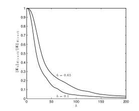
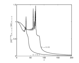
Fig. 1: $\left\|\mathbf{E}_{h}\right\|_{H(\operatorname{\mathbf{curl}},\mathcal{T}_{h})}\big{/}\left\|\mathbf{E}\right\|_{H(\operatorname{\mathbf{curl}},\mathcal{T}_{h})}$ (left) and $\left\|\mathbf{E}_{h}^{\mathrm{EEM}}\right\|_{H(\operatorname{\mathbf{curl}},\mathcal{T}_{h})}\big{/}\left\|\mathbf{E}\right\|_{H(\operatorname{\mathbf{curl}},\mathcal{T}_{h})}$ (right) versus $k$ for $k=1,2,\cdots,200$ with $h=0.1,0.05$, respectively.

6.2 Error estimates

In this subsection, we use the same penalty parameters as given in (82). In the left graph of Figure 2, the relative $H(\operatorname{\mathbf{curl}})$-error of the IPDG solution and the relative $H(\operatorname{\mathbf{curl}})$-error of the edge element interpolant are displayed in one plot. When the mesh size is decreasing, the relative error of the IPDG solution stays around $100\%$ before it is less than $100\%$, then decays slowly on a range increasing with $k$, and then decays at a rate greater than $-1$ in the log-log scale but converges as fast as the edge element interpolant (with slope $-1$) for small $h$. The relative error grows with $k$ along line $kh=1.$ By contrast, as shown in the right of Figure 2, the relative error of the finite element solution first stay around $100\%$ but oscillates for large $k$, then decays at a rate greater than $-1$ in the log-log scale but converges as fast as the edge element interpolant (with slope $-1$) for small $h$. The relative error of the edge element solution also grows with $k$ along line $kh=1$.

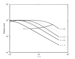
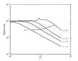
Fig. 2: Left graph: the relative error of the IPDG solution with parameters given in (82) (solid) and the relative error of the edge element interpolant (dotted) in $H(\operatorname{\mathbf{curl}})$-norm for $k=5,k=10,k=15,$ and $k=30$, respectively. The dashed line gives reference slope of $-1$. Right graph: corresponding plots for edge element solutions.

Unlike the error of the edge element interpolant, both the error of the IPDG solution and that of the edge element solution are not controlled by the magnitude of $kh$ as indicated by the two graphs in Figure 3. It is shown that when $h$ is determined according to the “rule of thumb”, the relative error of the IPDG solution keeps less than $100\%$ which means that the IPDG solution has some accuracy even for large $k$, while the edge element solution is unusable for large $k$. We remark that the accuracy of the IPDG solution can be further improved by tuning the penalty parameter ${\rm\mathbf{i}}\gamma_{1}$, see Subsection 6.3 below.

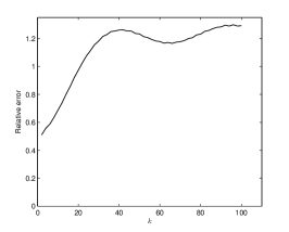
Fig. 3: The relative error of the IPDG solution (left) with parameters given in (82) and that of the edge element solution (right) in $H(\operatorname{\mathbf{curl}})$-norm computed for $k=2,4,\cdots,72$ with mesh size $h$ determined by $kh=2$.

Next we verify more precisely the pollution errors. To do so, we recall the definition of the critical mesh size with respect to a given relative tolerance (cf. [23, Definition 7.1]).

Definition 13.

Given a relative tolerance $\varepsilon$ and a wave number $k$, the critical mesh size $h(k,\varepsilon)$ with respect to the relative tolerance $\varepsilon$ is defined by the maximum mesh size such that the relative error of the IPDG solution (or the edge element solution) in $H(\operatorname{\mathbf{curl}})$-norm is less than or equal to $\varepsilon$.

It is clear that, if the pollution terms are of order $k^{\beta}h^{\alpha}$, then $h(k,\varepsilon)$ should be proportional to $k^{-\beta/\alpha}$ for $k$ large enough. Figure 4 which plots $h(k,0.5)$ versus $k$ for the IPDG solution (left) with parameters given in (82) and for the edge element solution (right), respectively. They all decay at a rate of $O(k^{-3/2})$, just like the linear FEM for the Helmholtz problem (cf. [23]). The results of this subsection indicate that both methods satisfy the following pre-asymptotic error bounds (cf. Remark 5.3(a)):

$$\Bigl{\{}\left\|\mathbf{E}-\mathbf{E}_{h}\right\|_{H(\operatorname{\mathbf{curl}},\mathcal{T}_{h})},\quad\left\|\mathbf{E}-\mathbf{E}_{h}^{\mathrm{EEM}}\right\|_{H(\operatorname{\mathbf{curl}},\Omega)}\Bigr{\}}\leq C_{1}kh+C_{2}k^{3}h^{2}.$$

Fig. 4: $h(k,0.5)$ versus $k$ for the IPDG solution (left) with parameters given in (82) and for the edge element solution (right), respectively. The dotted lines give lines of slope $-1.5$ in the log-log scale.

6.3 Reduction of the pollution effect

In this subsection, we show that appropriate choice of the penalty parameters can significantly reduce the pollution error of the IPDG method. We use the following parameters:

(83) $$\gamma_{0,\mathcal{F}}\equiv\gamma_{0}=100\quad\text{ and }\quad{\rm\mathbf{i}}\gamma_{1,\mathcal{F}}\equiv{\rm\mathbf{i}}\gamma_{1}=0.08+0.01{\rm\mathbf{i}}\quad\forall\mathcal{F}\in\mathcal{E}_{h}^{I}.$$

We remark that ${\rm\mathbf{i}}\gamma_{1,\mathcal{F}}$ is simply chosen from the set $\left\{0.01(p+q{\rm\mathbf{i}}),-50\leq p,q\leq 50\right\}$ to minimize the relative error of the IPDG solution in $H(\operatorname{\mathbf{curl}})$-norm with $\gamma_{0}=100$ for wave number $k=20$ and mesh size $h=1/10$. The optimal penalty parameter can also be obtained by the dispersion analysis (cf. [1]) and will be considered in a future work.

The relative error of the IPDG solution with parameters given in (83) and the relative error of the edge element interpolant are displayed in the left graph of Figure 5. The IPDG method with parameters given in (83) is much better than both the IPDG method using parameters given in (82) and the EEM (cf. Figure 2 and Figure 3). The relative error does not increase much with the change of $k$ along line $kh=1$ for $k\leq 30$. But this does not mean that the pollution error has been eliminated.

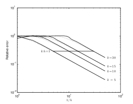
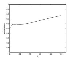
Fig. 5: Left graph: the relative error of the IPDG solution with parameters given in (83) (solid) and the relative error of the edge element interpolant (dotted) in $H(\operatorname{\mathbf{curl}})$-norm for $k=5,k=10,k=15,$ and $k=30$, respectively. Right graph: the relative error of the IPDG solution with parameters given in (83) in $H(\operatorname{\mathbf{curl}})$-norm computed for $k=2,4,\cdots,72$ with mesh size $h$ determined by $kh=2$.

For more detailed observation, the relative error of the IPDG solution with parameters given in (83) in $H(\operatorname{\mathbf{curl}})$-norm computed for $k=2,4,\cdots,72$ with mesh size $h$ determined by $kh=2$, are plotted in the right graph of Figure 5. It is shown that the pollution error is reduced significantly.

Figure 6 plots $h(k,0.5)$, the critical mesh size with respect to the relative tolerance $50\%$, versus $k$ for the IPDG method with parameters given in (83). We recall that $h(k,0.5)$ is the maximum mesh size such that the relative error of the IPDG solution in $H(\operatorname{\mathbf{curl}})$-norm is less than or equal to $50\%$. The decreasing rate of $h(k,0.5)$ in the log-log scale is less than $-1.5$, which means that the pollution effect is reduced.

Fig. 6: $h(k,0.5)$ versus $k$ for the IPDG method with parameters given in (83). The dotted line gives a line of slope $-1.5$ in the log-log scale.

For more detailed comparison between the continuous interior penalty finite element method (CIP-FEM) and the FEM, we consider the problem (80)–(81) with wave number $k=36$. The real parts of $\mathbf{E}_{hx}(0.5,0.5,z)$ with parameters given in (83) (left, solid), $\mathbf{E}_{hx}^{\mathrm{EEM}}(0.5,0.5,z)$ (right, solid), and $\mathbf{E}_{x}(0.5,$ $0.5,z)$ (dotted) with mesh sizes $h=1/18$ and $1/36$ are plotted in Figure 7. Here $\mathbf{E}_{hx}$, $\mathbf{E}_{hx}^{\mathrm{EEM}}$, and $\mathbf{E}_{x}$ are the $x$ components of the IPDG solution, the edge element solution, and the exact solution, respectively. The shape of the IPDG solution is roughly same as that of the exact solution for $h=1/18$ and matches very well for $h=1/36$. While the edge element solution has a wrong shape for $h=1/18$ and $z>0.5$ and has a correct shape for $h=1/36$ but suffers an apparent phase error.

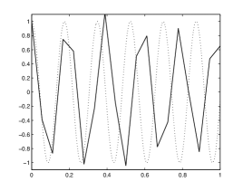
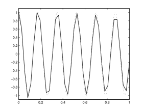
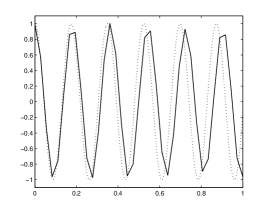
Fig. 7: The real parts of $\mathbf{E}_{hx}(0.5,0.5,z)$ with parameters given in (83) (left, solid), $\mathbf{E}_{hx}^{\mathrm{EEM}}(0.5,0.5,z)$ (right, solid), and $\mathbf{E}_{x}(0.5,0.5,z)$ (dotted) for $k=36$ and $h=1/18$, $1/36$, respectively.

Table 1 shows the numbers of total DOFs needed for $50$% relative errors in $H(\operatorname{\mathbf{curl}})$-norm for the edge element interpolant, the IPDG solution with parameters given in (83), and the edge element solution, respectively. The IPDG method needs less DOFs than the EEM does for $k\geq 10$ and much less for large wave number $k$.

$k$	10	20	30	40	50
Interpolation	1,764	12,168	33,048	79,488	141,288
IPDG	2,592	20,736	69,984	187,500	393,216
EEM	2,688	45,600	249,900	876,408	2,398,488

Table 1: Numbers of total DOFs needed for 50% relative errors in $H(\operatorname{\mathbf{curl}})$-norm for the edge element interpolant, the IPDG solution with parameters given in (83), and the edge element solution respectively.

Acknowledgments. The authors would like to thank Dr. Huangxin Chen of Xiamen University of China for his helpful suggestions on the construction and analysis of the $\mathbf{H}(\operatorname{\mathbf{curl}},\Omega)$-elliptic projection in section 5.1.

Appendix A Proof of (71)

The proof follows the same lines as those given in [15, pages 502–505] and in [17, 24]. Let

$$U_{h}=\bigl{\{}v_{h}\in H^{1}(\Omega);\,v_{h}|_{K}\in P_{2}(K),\forall K\in\mathcal{T}_{h}\bigr{\}}$$

be the $H^{1}$-conforming linear finite element space. It follows from (53) that $\mathbf{E}-\widetilde{\mathbf{E}}_{h}$ is discrete divergence-free, that is,

$$\bigl{(}\mathbf{E}-\widetilde{\mathbf{E}}_{h},{\rm NewA}\varphi_{h}\bigr{)}_{\Omega}=0\qquad\forall\varphi_{h}\in U_{h}.$$

Notice that $\boldsymbol{\Phi}_{h}^{c}\in\mathbf{V}_{h}\cap\mathbf{H}(\operatorname{\mathbf{curl}},\Omega)$, we have the following discrete Helmholtz decomposition of $\boldsymbol{\Phi}_{h}^{c}$:

(84) $$\boldsymbol{\Phi}_{h}^{c}=\mathbf{w}_{h}+{\rm NewA}r_{h},$$

where $r_{h}\in U_{h}$ and $\mathbf{w}_{h}\in\mathbf{V}_{h}\cap\mathbf{H}(\operatorname{\mathbf{curl}},\Omega)$ is also discrete divergence-free. It is easy to check that

$$\|{\rm NewA}r_{h}\|_{\mathbf{L}^{2}(\Omega)}\leq\|\boldsymbol{\Phi}_{h}^{c}\|_{\mathbf{L}^{2}(\Omega)},\qquad\|\mathbf{w}_{h}\|_{\mathbf{L}^{2}(\Omega)}\lesssim\|\boldsymbol{\Phi}_{h}^{c}\|_{\mathbf{L}^{2}(\Omega)}.$$

Then from [17, Lemma 7.6] and on noting that the domain $\Omega$ is convex, there exists $\mathbf{w}\in\mathbf{H}^{1}(\Omega)$ such that $\mathbf{w}\cdot\mathbf{n}=\mathbf{0}$ on $\Gamma$ and

(85) $$\operatorname{\mathbf{curl}}\mathbf{w}=\operatorname{\mathbf{curl}}\mathbf{w}_{h},\quad{\rm div\,}\mathbf{w}=0,\quad\|\mathbf{w}_{h}-\mathbf{w}\|_{\mathbf{L}^{2}(\Omega)}\lesssim h\|\operatorname{\mathbf{curl}}\boldsymbol{\Phi}_{h}^{c}\|_{\mathbf{L}^{2}(\Omega)}.$$

Thus, it follows from the identity

$$\bigl{(}\mathbf{E}-\widetilde{\mathbf{E}}_{h},\boldsymbol{\Phi}_{h}^{c}\bigr{)}_{\Omega}=\bigl{(}\mathbf{E}-\widetilde{\mathbf{E}}_{h},\mathbf{w}_{h}\bigr{)}_{\Omega}=\bigl{(}\mathbf{E}-\widetilde{\mathbf{E}}_{h},\mathbf{w}_{h}-\mathbf{w}\bigr{)}_{\Omega}+\bigl{(}\mathbf{E}-\widetilde{\mathbf{E}}_{h},\mathbf{w}\bigr{)}_{\Omega}$$

that

(86) $$-\frac{\bigl{(}\mathbf{E}-\widetilde{\mathbf{E}}_{h},\boldsymbol{\Phi}_{h}^{c}\bigr{)}_{\Omega}}{\|\mathbf{E}-\widetilde{\mathbf{E}}_{h}\|_{\mathbf{L}^{2}(\Omega)}} \leq\|\mathbf{w}_{h}-\mathbf{w}\|_{\mathbf{L}^{2}(\Omega)}+\|\mathbf{w}\|_{\mathbf{L}^{2}(\Omega)}$$

$$\lesssim h\|\operatorname{\mathbf{curl}}\boldsymbol{\Phi}_{h}^{c}\|_{\mathbf{L}^{2}(\Omega)}+\|\mathbf{w}\|_{\mathbf{L}^{2}(\Omega)}.$$

The first term on the right-hand side of (86) can be bounded as follows:

(87) $$h\|\operatorname{\mathbf{curl}}\boldsymbol{\Phi}_{h}^{c}\|_{\mathbf{L}^{2}(\Omega)}=h\|\operatorname{\mathbf{curl}}(\widehat{\mathbf{E}}_{h}-\mathbf{E}+\mathbf{E}-\widetilde{\mathbf{E}}_{h}+\boldsymbol{\Phi}_{h}-\boldsymbol{\Phi}_{h}^{c})\|_{\mathbf{L}^{2}(\Omega)}$$

$$\leq h\|\widehat{\mathbf{E}}_{h}-\mathbf{E}\|_{\mathbf{H}(\operatorname{\mathbf{curl}},\Omega)}+h\|\mathbf{E}-\widetilde{\mathbf{E}}_{h}\|_{DG}+h\|\operatorname{\mathbf{curl}}(\boldsymbol{\Phi}_{h}-\boldsymbol{\Phi}_{h}^{c})\|_{\mathbf{L}^{2}(\mathcal{T}_{h})}\lesssim h^{2}\mathcal{R}(\mathbf{E}).$$

where we have used (56), (62), and (69) to derive the last inequality.

To estimate $\|\mathbf{w}\|_{\mathbf{L}^{2}(\Omega)}$, we appeal to a duality argument to be described next. Let $\mathbf{z}$ be the solution of the following auxiliary problem:

(88) $$\operatorname{\mathbf{curl}}\operatorname{\mathbf{curl}}\mathbf{z}+\mathbf{z} =\mathbf{w}\quad\mbox{in }\Omega,\qquad\operatorname{\mathbf{curl}}\mathbf{z}\times\boldsymbol{\nu}=\mathbf{0}\quad\mbox{on }\Gamma:=\partial\Omega.$$

Noting that $\Omega$ is convex, the above problem attains a unique solution $\mathbf{z}\in\mathbf{H}^{1}(\operatorname{\mathbf{curl}},\Omega)$ and satisfies the following regularity estimate (cf. [13, 17])

(89) $$\|\mathbf{z}\|_{\mathbf{H}^{1}(\operatorname{\mathbf{curl}},\Omega)}\lesssim\|\mathbf{w}\|_{\mathbf{L}^{2}(\Omega)}.$$

Define sesquilinear forms

$$A(\mathbf{u},\mathbf{v}) :=(\operatorname{\mathbf{curl}}\mathbf{u},\operatorname{\mathbf{curl}}\mathbf{v})_{\Omega}+(\mathbf{u},\mathbf{v})_{\Omega}\qquad\forall\mathbf{u},\mathbf{v}\in\hat{\boldsymbol{\mathcal{V}}},$$

$$A_{h}(\mathbf{u},\mathbf{v}) :=b_{h}(\mathbf{u},\mathbf{v})+(\mathbf{u},\mathbf{v})_{\Omega}\qquad\forall\mathbf{u},\mathbf{v}\in\mathbf{V}.$$

Let $\mathbf{z}_{h}^{c}\in\mathbf{V}_{h}\cap\mathbf{H}(\operatorname{\mathbf{curl}},\Omega)$ and $\mathbf{z}_{h}\in\mathbf{V}_{h}$ denote the edge finite element approximation and the IPDG approximation to $\mathbf{z}$, respectively, that is,

$$A(\mathbf{v}_{h},\mathbf{z}_{h}^{c}) =(\mathbf{v}_{h},\mathbf{w})_{\Omega}\qquad\forall\mathbf{v}_{h}\in\mathbf{V}_{h}\cap\mathbf{H}(\operatorname{\mathbf{curl}},\Omega),$$

$$A_{h}(\mathbf{v}_{h},\mathbf{z}_{h}) =(\mathbf{v}_{h},\mathbf{w})_{\Omega}\qquad\forall\mathbf{v}_{h}\in\mathbf{V}_{h}.$$

It can be shown that there hold the following estimates (cf. (56)):

$$\|\mathbf{z}-\mathbf{z}_{h}^{c}\|_{\mathbf{H}(\operatorname{\mathbf{curl}},\Omega)} \lesssim h\,\|\mathbf{z}\|_{\mathbf{H}^{1}(\operatorname{\mathbf{curl}},\Omega)}\lesssim h\,\|\mathbf{w}\|_{\mathbf{L}^{2}(\Omega)},$$

$$\|{\hskip-1.3pt}|\mathbf{z}-\mathbf{z}_{h}^{c}|{\hskip-1.3pt}\|_{DG},\quad\|{\hskip-1.3pt}|\mathbf{z}-\mathbf{z}_{h}|{\hskip-1.3pt}\|_{DG} \lesssim h\,(1+\gamma_{1})^{\frac{1}{2}}\|\mathbf{z}\|_{\mathbf{H}^{1}(\operatorname{\mathbf{curl}},\Omega)}\lesssim h\,(1+\gamma_{1})^{\frac{1}{2}}\|\mathbf{w}\|_{\mathbf{L}^{2}(\Omega)}.$$

Since

$$\|\mathbf{w}\|_{\mathbf{L}^{2}(\Omega)}^{2} =A(\mathbf{w},\mathbf{z})=A(\mathbf{w},\mathbf{z}-\mathbf{z}_{h}^{c})+A(\mathbf{w},\mathbf{z}_{h}^{c}),$$

on noting that $\mathbf{w},\mathbf{w}_{h}\in\mathbf{H}(\operatorname{\mathbf{curl}},\Omega)$, from (85) and (87), we have

$$A(\mathbf{w},\mathbf{z}-\mathbf{z}_{h}^{c}) =A(\mathbf{w}-\mathbf{w}_{h},\mathbf{z}-\mathbf{z}_{h}^{c})=(\mathbf{w}-\mathbf{w}_{h},\mathbf{z}-\mathbf{z}_{h}^{c})_{\Omega}$$

$$\lesssim h\|\operatorname{\mathbf{curl}}\boldsymbol{\Phi}_{h}^{c}\|_{\mathbf{L}^{2}(\Omega)}\,h\,\|\mathbf{w}\|_{\mathbf{L}^{2}(\Omega)}\lesssim h^{3}\mathcal{R}(\mathbf{E})\|\mathbf{w}\|_{\mathbf{L}^{2}(\Omega)}.$$

On the other hand,

$$A(\mathbf{w},\mathbf{z}_{h}^{c}) =(\operatorname{\mathbf{curl}}\mathbf{w},\operatorname{\mathbf{curl}}\mathbf{z}_{h}^{c})_{\Omega}+(\mathbf{w},\mathbf{z}_{h}^{c})_{\Omega}=\bigl{(}\operatorname{\mathbf{curl}}\boldsymbol{\Phi}_{h}^{c},\operatorname{\mathbf{curl}}\mathbf{z}_{h}^{c}\bigr{)}_{\Omega}+(\mathbf{w},\mathbf{z}_{h}^{c})_{\Omega}$$

$$=A(\boldsymbol{\Phi}_{h}^{c},\mathbf{z}_{h}^{c})+\bigl{(}\mathbf{w}-(\mathbf{w}_{h}+{\rm NewA}r_{h}),\mathbf{z}_{h}^{c}\bigr{)}_{\Omega}=A(\boldsymbol{\Phi}_{h}^{c},\mathbf{z}_{h}^{c})+(\mathbf{w}-\mathbf{w}_{h},\mathbf{z}_{h}^{c})_{\Omega}.$$

From the definitions of $A,A_{h}$ and $b_{h}$, we get

$$A(\boldsymbol{\Phi}_{h}^{c},\mathbf{z}_{h}^{c})=A_{h}(\boldsymbol{\Phi}_{h}^{c},\mathbf{z}_{h}^{c})+{\rm\mathbf{i}}J_{1}(\boldsymbol{\Phi}_{h}^{c},\mathbf{z}_{h}^{c})$$

$$\quad=A_{h}(\mathbf{E}-\widehat{\mathbf{E}}_{h},\mathbf{z}_{h}^{c})+A_{h}(\widetilde{\mathbf{E}}_{h}-\mathbf{E},\mathbf{z}_{h}^{c})+A_{h}(\boldsymbol{\Phi}_{h}^{c}-\boldsymbol{\Phi}_{h},\mathbf{z}_{h}^{c})+{\rm\mathbf{i}}J_{1}(\boldsymbol{\Phi}_{h}^{c},\mathbf{z}_{h}^{c})$$

$$\quad=A_{h}(\mathbf{E}-\widehat{\mathbf{E}}_{h},\mathbf{z}_{h}^{c})+A_{h}(\boldsymbol{\Phi}_{h}^{c}-\boldsymbol{\Phi}_{h},\mathbf{z}_{h}^{c})+{\rm\mathbf{i}}J_{1}(\boldsymbol{\Phi}_{h}^{c},\mathbf{z}_{h}^{c}-\mathbf{z}).$$

Therefore

$$A(\mathbf{w},\mathbf{z}_{h}^{c})= A_{h}(\mathbf{E}-\widehat{\mathbf{E}}_{h},\mathbf{z}_{h}^{c}-\mathbf{z})+A_{h}(\mathbf{E}-\widehat{\mathbf{E}}_{h},\mathbf{z})+A_{h}(\boldsymbol{\Phi}_{h}^{c}-\boldsymbol{\Phi}_{h},\mathbf{z}_{h}^{c}-\mathbf{z}+\mathbf{z}-\mathbf{z}_{h})$$

$$+A_{h}(\boldsymbol{\Phi}_{h}^{c}-\boldsymbol{\Phi}_{h},\mathbf{z}_{h})+{\rm\mathbf{i}}J_{1}(\boldsymbol{\Phi}_{h}^{c},\mathbf{z}_{h}^{c}-\mathbf{z})+(\mathbf{w}-\mathbf{w}_{h},\mathbf{z}_{h}^{c})_{\Omega}.$$

Since

$$A_{h}(\mathbf{E}-\widehat{\mathbf{E}}_{h},\mathbf{z})=(\mathbf{E}-\widehat{\mathbf{E}}_{h},\mathbf{w})_{\Omega},\qquad A_{h}(\boldsymbol{\Phi}_{h}^{c}-\boldsymbol{\Phi}_{h},\mathbf{z}_{h})=(\boldsymbol{\Phi}_{h}^{c}-\boldsymbol{\Phi}_{h},\mathbf{w})_{\Omega},$$

we have from Lemma 8 and the local trace inequality,

$$A(\mathbf{w},\mathbf{z}_{h}^{c})\lesssim\|{\hskip-1.3pt}|\mathbf{E}-\widehat{\mathbf{E}}_{h}|{\hskip-1.3pt}\|_{DG}\|{\hskip-1.3pt}|\mathbf{z}_{h}^{c}-\mathbf{z}|{\hskip-1.3pt}\|_{DG}+\|\mathbf{E}-\widehat{\mathbf{E}}_{h}\|_{\mathbf{L}^{2}(\Omega)}\|\mathbf{w}\|_{\mathbf{L}^{2}(\Omega)}$$

$$\hskip 46.0pt+\|{\hskip-1.3pt}|\boldsymbol{\Phi}_{h}^{c}-\boldsymbol{\Phi}_{h}|{\hskip-1.3pt}\|_{DG}\big{(}\|{\hskip-1.3pt}|\mathbf{z}_{h}^{c}-\mathbf{z}|{\hskip-1.3pt}\|_{DG}+\|{\hskip-1.3pt}|\mathbf{z}-\mathbf{z}_{h}|{\hskip-1.3pt}\|_{DG}\big{)}+\|\boldsymbol{\Phi}_{h}^{c}-\boldsymbol{\Phi}_{h}\|_{\mathbf{L}^{2}(\Omega)}\|\mathbf{w}\|_{\mathbf{L}^{2}(\Omega)}$$

$$\hskip 46.0pt+\gamma_{1}\|\operatorname{\mathbf{curl}}\boldsymbol{\Phi}_{h}^{c}\|_{\mathbf{L}^{2}(\Omega)}\big{(}\|\operatorname{\mathbf{curl}}(\mathbf{z}_{h}^{c}-\mathbf{z})\|_{\mathbf{L}^{2}(\Omega)}+h\|\operatorname{\mathbf{curl}}(\mathbf{z}_{h}^{c}-\mathbf{z})\|_{H^{1}(\mathcal{T}_{h})}\big{)}$$

$$\hskip 46.0pt+\|\mathbf{w}-\mathbf{w}_{h}\|_{\mathbf{L}^{2}(\Omega)}\|\mathbf{z}_{h}^{c}\|_{\mathbf{L}^{2}(\Omega)}$$

$$\lesssim\|\mathbf{w}\|_{\mathbf{L}^{2}(\Omega)}\Big{(}h\,(1+\gamma_{1})^{\frac{1}{2}}\|{\hskip-1.3pt}|\mathbf{E}-\widehat{\mathbf{E}}_{h}|{\hskip-1.3pt}\|_{DG}+\|\mathbf{E}-\widehat{\mathbf{E}}_{h}\|_{\mathbf{L}^{2}(\Omega)}+h\,(1+\gamma_{1})^{\frac{1}{2}}\|{\hskip-1.3pt}|\boldsymbol{\Phi}_{h}^{c}-\boldsymbol{\Phi}_{h}|{\hskip-1.3pt}\|_{DG}$$

$$\quad+\|\boldsymbol{\Phi}_{h}^{c}-\boldsymbol{\Phi}_{h}\|_{\mathbf{L}^{2}(\Omega)}+\gamma_{1}h\|\operatorname{\mathbf{curl}}\boldsymbol{\Phi}_{h}^{c}\|_{\mathbf{L}^{2}(\Omega)}+h\|\operatorname{\mathbf{curl}}\boldsymbol{\Phi}_{h}^{c}\|_{\mathbf{L}^{2}(\Omega)}\Big{)}.$$

Moreover, from (69), (66), $\gamma_{0}\gtrsim 1$, and the local trace inequality, we get

$$\|{\hskip-1.3pt}|\boldsymbol{\Phi}_{h}^{c}-\boldsymbol{\Phi}_{h}|{\hskip-1.3pt}\|_{DG} \lesssim(1+\gamma_{1})^{\frac{1}{2}}\|\operatorname{\mathbf{curl}}(\boldsymbol{\Phi}_{h}-\boldsymbol{\Phi}_{h}^{c})\|_{\mathbf{L}^{2}(\mathcal{T}_{h})}+\|\boldsymbol{\Phi}_{h}\|_{DG}+\|\boldsymbol{\Phi}_{h}^{c}-\boldsymbol{\Phi}_{h}\|_{\mathbf{L}^{2}(\Omega)}$$

$$\lesssim(1+\gamma_{1})^{\frac{1}{2}}h\,\mathcal{R}(\mathbf{E}).$$

Thus, it follows from (66), (87), (69), and the above estimate that

$$A(\mathbf{w},\mathbf{z}_{h}^{c})\lesssim (1+\gamma_{1})h^{2}\mathcal{R}(\mathbf{E})\|\mathbf{w}\|_{\mathbf{L}^{2}(\Omega)}.$$

Then we obtain the following estimates for $\|\mathbf{w}\|_{\mathbf{L}^{2}(\Omega)}$:

$$\|\mathbf{w}\|_{\mathbf{L}^{2}(\Omega)}\lesssim(1+\gamma_{1})h^{2}\mathcal{R}(\mathbf{E}),$$

which together with (86) and (87) implies that (71) holds. The proof is complete.