Evolution of quantum correlations in a two-atom system

Abstract

We discuss the evolution of quantum correlations for a system of two two-level atoms interacting with a common reservoir. The Markovian master equation is used to describe the evolution of various measures of quantum correlations. It is shown that different measures of quantum correlations exhibit qualitatively different behaviour in their evolution.

1 Introduction

It is now well established that quantum entanglement, which is a measure of quantum correlations, is a necessary resource to perform some quantum information algorithms [1]. However, it has been realized that quantum entanglement does not include all quantum correlations, and there are separable states which exhibit quantum correlations different from entanglement. It became important to recognise the nature of correlations and properly discriminate quantum correlations from the classical ones. A number of measures of quantum correlations has been introduced, and the most popular of them is quantum discord [2, 3] (see also the review [4] and papers cited there). It is crucial, from the point of view of future application, to know how quantum correlations evolve in time when a multipartite system interacts with the dissipative environment.

The time evolution of entanglement for a system of two qubits, or two two-level atoms, can be qualitatively described for various physical situations, and it has been studied extensively in recent years [5, 6, 7, 8, 9, 10, 11, 12]. A lot of discussion has been devoted to the problem of disentanglement of the two-qubit system in a finite time, despite the fact that all the matrix elements of the two-atom system decay only asymptotically. Yu and Eberly [9] coined the name “entanglement sudden death” (ESD) to the process of finite-time disentanglement. ESD has recently been confirmed experimentally [10]. Another problem related to the entanglement evolution that attracted attention is the evolution of the entangled qubits interacting with the non-Markovian reservoirs [13, 14, 15]. It has also been shown that squeezed reservoir leads to the steady-state entanglement [16] and revivals of entanglement [17].

Beside entanglement, a considerable amount of attention has been paid in recent years to quantum discord. Generally, quantum discord is difficult to calculate because it requires the optimisation procedure which usually amounts to extensive numerical calculations. In case of two qubits analytical results can be obtained for some specific families of states, like Bell-diagonal states or states having maximally-mixed marginals [18]. Another interesting family of states is a family of the two-qubit X-states, which are of interest here. Ali et al. [19] reported a closed form solution for quantum discord of the X states. However, it turned out that their algorithm is not universal. Lu et al. [20] have proven that the universal set of orthogonal projective measurements cannot be found for the full family of X states. Some counterexamples have been given in [20, 21]. Chen et al. [21], however, confirmed applicability of the algorithm for several special cases of X states. Lu et al. have found that the probability distribution of measurements is centralised around a specific von Neumann measurement, which they called the maximal-correlation-direction measurement. This observation justifies the Ali et al. algorithm in a statistical sense, because, it turns out that for 99.4% of cases of numerically generated X states the algorithm gives correct results. The situation with arbitrary two-qubit states is more complicated and the best what has been achieved so far are the two transcendental equations obtained by Girolami and Adesso [22] which must be solved numerically to get quantum discord.

Dakić et al. [23] have introduced another measure of quantum correlation based on the Hilbert-Schmidt distance measure, which is called geometric discord. The advantage of this measure is that it allows for getting analytical formulas for general two-qubit states. Girolami and Adesso [24] introduced the so called observable measure of bipartite quantum correlation which is a lower bound to the geometric discord. Behaviour of the geometric discord under decoherence has been studied in [25]. Recently Bellomo et al. [26] compared the dynamics of geometric and entropic quantifiers of the different kinds of correlations in a non-Markovian open two-qubit system under local dephasing.

In this paper we study the evolution of concurrence (a measure of entanglement), quantum discord and geometric discord in a system of two two-level atoms interacting with a common reservoir being in a vacuum state. The evolution of the system is described by the Markovian master equation introduced by Lehmberg [27] and Agarwal [28], taking into account the cooperative behaviour of the atoms. It is shown that different measures of quantum correlations evolve in time quite differently. We compare their evolution for a family of pure initial states. Since the evolution of the system is described by a realistic master equation, which is a good testing ground for studying physical processes involving two atoms, we believe the results obtained shed new light on understanding quantum correlations.

2 Master equation

We consider a system of two two-level atoms, $A$ and $B$, with ground states $|g_{i}\rangle$ and excited states $|e_{i}\rangle$ ($i=A,B$) connected by dipole transition moments $\bm{\mu}_{i}$. The atoms are located at fixed positions $r_{A}$ and $r_{B}$ and coupled to all modes of the electromagnetic field being in the vacuum state.

The reduced two-atom density matrix evolves in time according to the Markovian master equation given by [27, 28, 29]

$$\frac{\partial\rho}{\partial t} = -i\sum_{i=1}^{2}\omega_{i}\left[S^{z}_{i},\rho\right]-i\sum_{i\neq j}^{2}{\Omega_{ij}}\left[S^{+}_{i}S^{-}_{j},\rho\right]$$ (1)

$$-\frac{1}{2}\sum_{i,j=1}^{2}{\Gamma_{ij}}\left(\rho S_{i}^{+}S_{j}^{-}+S_{i}^{+}S_{j}^{-}\rho-2S_{j}^{-}\rho S_{i}^{+}\right)$$

where $S_{i}^{+}$ ($S_{i}^{-}$) are the raising (lowering) operators, and $S^{z}_{i}$ is the energy operator of the $i$th atom, $\Gamma_{ii}\equiv\Gamma$ are the spontaneous decay rates. We assume that the two atoms are identical. The parameters $\Gamma_{ij}$ and $\Omega_{ij}\ (i\neq j)$ depend on the distance between the atoms and describe the collective damping and the dipole-dipole interaction defined, respectively, by

$$\Gamma_{ij}=\frac{3}{2}\Gamma\left(\frac{\sin kr_{ij}}{kr_{ij}}+\frac{\cos kr_{ij}}{\left(kr_{ij}\right)^{2}}-\frac{\sin kr_{ij}}{\left(kr_{ij}\right)^{3}}\right),$$ (2)

and

$$\Omega_{ij}=\frac{3}{4}\Gamma\left(-\frac{\cos kr_{ij}}{kr_{ij}}+\frac{\sin kr_{ij}}{\left(kr_{ij}\right)^{2}}+\frac{\cos kr_{ij}}{\left(kr_{ij}\right)^{3}}\right),$$ (3)

where $k=\omega_{0}/c$, and $r_{ij}$ is the distance between the atoms. Here, we assume, with no loss of generality, that the atomic dipole moments are parallel to each other and are polarised in the direction perpendicular to the interatomic axis.

To describe the evolution of the two-qubit system the standard basis of atomic product states can be used: $|1\rangle=|e_{A}\rangle\otimes|e_{B}\rangle$, $|2\rangle=|e_{A}\rangle\otimes|g_{B}\rangle$, $|3\rangle=|g_{A}\rangle\otimes|e_{B}\rangle$, $|4\rangle=|g_{A}\rangle\otimes|g_{B}\rangle$. It is easier, however, to find the solutions of the master equations when using instead of the standard basis, a basis of the collective states: $|e\rangle=|e_{A}\rangle\otimes|e_{B}\rangle$, $|s\rangle=\frac{1}{\sqrt{2}}\left(|e_{A}\rangle\otimes|g_{B}\rangle+|g_{B}\rangle\otimes|e_{B}\rangle\right)$, $|a\rangle=\frac{1}{\sqrt{2}}\left(|e_{A}\rangle\otimes|g_{B}\rangle-|g_{A}\rangle\otimes|e_{B}\rangle\right)$, $|g\rangle=|g_{A}\rangle\otimes|g_{B}\rangle$. The states $|s\rangle$ and $|a\rangle$ are the symmetric and antisymmetric states of the two-atom system. They are maximally entangled states, or Bell states of the two-atom system. Assuming that initially the system density matrix has the so called $X$ form, which is preserved during the evolution according to the master equation (1), and we get the following system of equations for the density matrix elements [29]

$$\rho_{ee}(t) = \rho_{ee}(0){\rm e}^{-2\Gamma t},$$

$$\rho_{ss}(t) = \rho_{ss}(0){\rm e}^{-\Gamma_{+}t}+\rho_{ee}(0)\frac{\Gamma_{+}}{\Gamma_{-}}\left[{\rm e}^{-\Gamma_{+}t}-{\rm e}^{-2\Gamma t}\right],$$

$$\rho_{aa}(t) = \rho_{aa}(0){\rm e}^{-\Gamma_{-}t}+\rho_{ee}(0)\frac{\Gamma_{-}}{\Gamma_{+}}\left[{\rm e}^{-\Gamma_{-}t}-{\rm e}^{-2\Gamma t}\right],$$ (4)

$$\rho_{as}(t) = \rho_{as}(0){\rm e}^{-(\Gamma+i2\Omega_{12})t},$$

$$\rho_{eg}(t) = \rho_{ge}(0){\rm e}^{-(\Gamma+2i\omega_{0})t},\$$

where $\Gamma_{\pm}=\Gamma\pm\Gamma_{AB}$. For calculating the quantum correlations measures we need the solutions for the density matrix elements in the standard product basis, which can be expressed in terms of the matrix elements (2) in the following way

$$\rho_{11}(t) = \rho_{ee}(t),$$

$$\rho_{14}(t) = \rho_{eg}(t),$$

$$\rho_{22}(t) = [\rho_{ss}(t)+\rho_{aa}(t)+\rho_{as}(t)+\rho_{sa}(t)]/2,$$ (5)

$$\rho_{33}(t) = [\rho_{ss}(t)+\rho_{aa}(t)+\rho_{as}(t)-\rho_{sa}(t)]/2,$$

$$\rho_{23}(t) = [\rho_{ss}(t)-\rho_{aa}(t)+\rho_{as}(t)-\rho_{sa}(t)]/2.$$

The solutions (2) and (2) are used to find the evolution of various measures of quantum correlations.

(a)
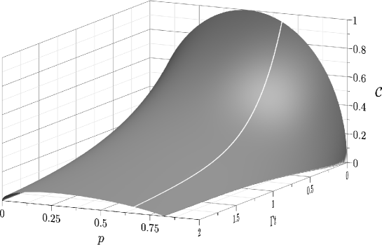
(b)
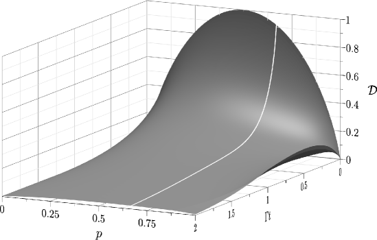
(c)

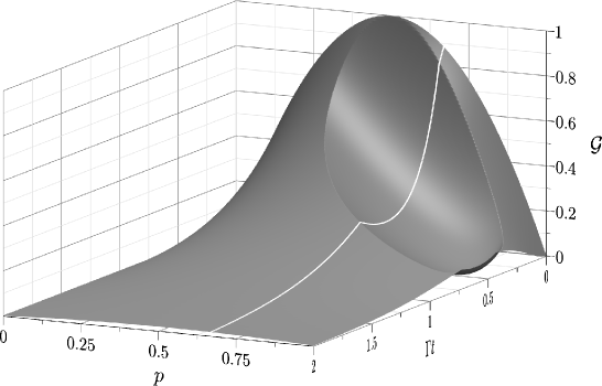
Figure 1: Evolution of concurrence (a), quantum discord (b), and geometric quantum discord (c), for the two-photon Bell-like state (13) and the interatomic distance $r_{AB}=\lambda/8$. The white lines show section of the surface for $p=2/3$.

3 Measures of quantum correlations

3.1 Entanglement

Probably the most celebrated and studied manifestation of quantum correlations is quantum entanglement. To quantify the entanglement, various entanglement measures have been introduced. We use here concurrence introduced by Wootters [30]. In the case of X states we consider, the concurrence can be calculated analytically, and it has the form [7]

$${\cal C}(t) = \max\left\{0,{\sf C}_{1}(t),{\sf C}_{2}(t)\right\}$$

$${\sf C}_{1}(t) = 2\left(|\rho_{14}(t)|-\sqrt{\rho_{22}(t)\rho_{33}(t)}\right)$$ (6)

$${\sf C}_{2}(t) = 2\left(|\rho_{23}(t)|-\sqrt{\rho_{11}(t)\rho_{44}(t)}\right)$$

Inserting into (3.1) the solutions (2) and (2), we find the values of ${\sf C}_{1}(t)$ and ${\sf C}_{2}(t)$, and whenever one of the two quantities becomes positive, there is a some degree of entanglement in the system.

(a)
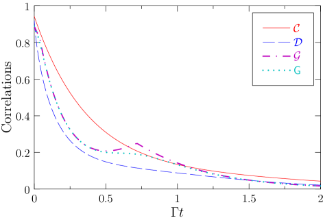
(b)

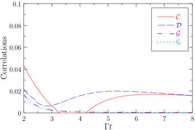
Figure 2: Evolution of correlations for the state (13) and interatomic distance $r_{AB}=\lambda/8$ for $p=2/3$. The evolution is split into two time regions (notice the different scales of both parts).

(a)
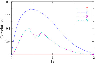
(b)

Figure 3: Same as Fig. 2, but for $p=1$, i.e. initially both atoms excited.

3.2 Quantum discord

To calculate quantum discord we use the algorithm introduced by Ali et al. [19], which works quite well in our case. We have checked for many numerically generated X states, for which the algorithm fails to find correct extremum, that the differences between the numerically found extrema and the values given by the algorithm are so small that they cannot be resolved in the scale of the figures. In our calculation, we assume that the measurement is performed on the subsystem $B$. For X state we have [2, 3, 19]

$${\cal D} = S(\rho^{B})-S(\rho)+\min\{{\cal K}_{1},{\cal K}_{2}\},$$

$${\cal K}_{1} = H\left[\frac{1}{2}\left(1+\sqrt{(s^{A}_{z})^{2}+4\eta^{2}}\right)\right],$$ (7)

$${\cal K}_{2} = -\sum_{i}\rho_{ii}\log_{2}\rho_{ii}-S(\rho^{B}),$$

where $S(\rho)$, $S(\rho^{B})$ mean the von Neumann entropy for the two-atom system and the subsystem $B$, respectively, $s_{z}^{A}={\rm Tr}[\rho\sigma^{A}_{z}]=\rho_{11}+\rho_{22}-\rho_{33}-\rho_{44}$ is the third component of the Bloch vector of the subsystem $A$, and $\eta=|\rho_{14}|+|\rho_{23}|$. $H(x)$ is the Shannon entropy.

3.3 Geometric quantum discord

Geometric quantum discord is defined as [23, 31]

$${\cal G} = 2\min_{{\cal X}}||\rho-{\cal X}||^{2}$$ (8)

where ${\cal X}$ is a set of zero-discord states, and $||\dots||$ denotes the Hilbert-Schmidt norm. The factor 2 in front has been introduced for normalisation. The general formula for the geometric quantum discord takes the form

$${\cal G} = \frac{1}{2}\left(||\vec{s}^{B}||^{2}+||T||^{2}-k_{max}\right)$$ (9)

where $\vec{s}^{B}$ is the Bloch vector for the subsystem $B$ (we assume that measurement is performed on subsystem $B$), and $k_{max}$ is the largest eigenvalue of the matrix

$$K=\vec{s}^{B}(\vec{s}^{B})^{t}+T^{t}T,$$ (10)

where the superscript $t$ means transposition.

For X states we have

$${\cal G} = \min\{{\cal G}_{1},{\cal G}_{2}\}$$

$${\cal G}_{1} = 4(|\rho_{14}|^{2}+|\rho_{23}|^{2})$$ (11)

$${\cal G}_{2} = 2(|\rho_{14}|^{2}-|\rho_{2}|^{2})^{2}+\frac{1}{2}\left[(s_{z}^{B})^{2}+T_{zz}^{2}\right]$$

where $s^{B}_{z}=\rho_{11}-\rho_{22}+\rho_{33}-\rho_{44}$ is the third component of the Bloch vector for the subsystem $B$ and $T_{ij}={\rm Tr}[\rho(\sigma^{A}_{i}\otimes\sigma_{j}^{B})$, ($i,j=x,y,z$), are elements of the correlation matrix.

The observable measure of Girolami and Adesso [24] is given by the formula

$${\sl G} = \frac{1}{6}\left[2{\rm Tr}(K)-\sqrt{6{\rm tr}(K^{2})-2\left[{\rm Tr}(K)\right]^{2}}\right]$$ (12)

with the matrix $K$ given by (10).

4 Evolution of quantum correlations

To compare the evolution of various measures of quantum correlations in a system of two two-level atoms governed by the master equation (1), we assume that the initial state is the Bell-like state

$$|\Psi\rangle=\sqrt{p}\,|1\rangle+\sqrt{1-p}\,|4\rangle$$ (13)

where $p$ is the population of the upper state $|1\rangle$. In Fig. 1 we illustrate the evolution of concurrence, quantum discord and geometric quantum discord for the whole range of values of $p$. For $p<1$ the state (13) is a superposition of the states $|1\rangle$ and $|4\rangle$ which has nonzero two-photon coherence $\rho_{14}$, while for $p=1$ it is a product state of both atoms excited. It is seen from Fig. 1 that the evolution of different measures of quantum correlations depends on the value of $p$ and shows essential differences, not only quantitative but also qualitative. The white line seen on the figures indicates the section of the surface at $p=2/3$. The evolution for this value of $p$ is illustrated in more details in Fig. 2. It has been shown before [11] that there is sudden death and revival of entanglement in the system for $p>0.5$, which is clearly seen in Fig. 2b. The other correlations do not exhibit sudden death, but there is an increase in quantum discord for $\Gamma t>2$. The most striking feature is the behaviour of geometric quantum discord with a deep crater for $\Gamma t<1$ as seen in Fig. 1c, and the cusp seen in Fig. 2a. The observable measure of geometric quantum discord given by (12) and shown in Fig. 2a smoothes out the cusp of geometric discord.

For $p=1$ the state (13) becomes the product state of both atoms being excited for which all the correlations are zero. However, as it is evident from Fig. 1, concurrence remains zero for some time, while the other correlations increase immediately after the start of the evolution. It is clearly evident from Fig. 3. For short times the quantum discord increases, reaches the maximum and goes down to the minimum in order to increase again to the subsequent maximum, and eventually it goes down to zero asymptotically. This behaviour has been reported in [32]. The concurrence remains zero up to $\Gamma t\sim 4$ and next abruptly becomes nonzero, the effect that has been referred to as sudden birth of entanglement [12]. Both revival of entanglement and the sudden birth of entanglement are due to collective behaviour of the two atoms when the interatomic distance is smaller than the wavelength of light emitted by individual atom [33, 11, 12]. Here we take the interatomic distance equal to $\lambda/8$.

From Fig. 3a it is seen that the geometric quantum discord has a minimum with sharp cusps, and the observable measure of geometric quantum discord, which is a lower bound for geometric quantum discord, is a really tight bound, except for the interval around the minimum, where the bound is not so tight. For this time interval geometric quantum discord behaves quite differently than quantum discord, and both differ from concurrence.

5 Conclusions

We have discussed the dynamics of various measures of quantum correlations in a two-atom system interacting with a common reservoir in a vacuum state. The evolution of the system is described by the Lehmberg-Agarwal Markovian master equation, which takes into account collective behaviour of the atoms. The collective spontaneous emission is a source of quantum correlations in the system. We have shown that the evolution of different measures of quantum correlations is qualitatively different, with a rather strange behaviour of the geometric discord. Some aspects of the evolution of quantum correlation in such a system has been studied in [34]. Recently Piani [35] has argued that the geometric discord is not a good measure for the quantumness of correlations.

References

References

- [1] Horodecki R, Horodecki P, Horodecki M and Horodecki K 2009 Rev. Mod. Phys. 81 865
- [2] Ollivier H and Zurek W H 2002 Phys. Rev. Lett. 88 017901
- [3] Henderson L and Vedral V 2001 J. Phys. A 34 6899
- [4] Modi K, Brodutch A, Cable H, Paterek T and Vedral V 2011 arXiv:1112.6238v1 (quant-ph)
- [5] Życzkowski K, Horodecki P, Horodecki M and Horodecki R 2001 Phys. Rev. A 65 012101
- [6] Jakóbczyk L 2002 J. Phys. A 35 6383
- [7] Ficek Z and Tanaś R 2003 J. Mod. Opt. 50 2765
- [8] Nicolosi S, Napoli A, Messina A and Petruccione F 2004 Phys. Rev. A 70 022511
- [9] Yu T and Eberly J H 2004 Phys. Rev. Lett. 93 140404
- [10] Almeida M P, de Melo F, Hor-Meyll M, Salles A, Walborn S P, Souto Ribeiro P H and Davidovich L 2007 Science 316 579
- [11] Ficek Z and Tanaś R 2006 Phys. Rev. A 74 024304
- [12] Ficek Z and Tanaś R 2008 Phys. Rev. A 77 054301
- [13] Bellomo B, Lo Franco R and Compagno G 2007 Phys. Rev. Lett. 99 160502
- [14] Cao X and Zheng H 2008 Phys. Rev. A 77 022320
- [15] Wang F, Zhang Z and Liang R 2008 Phys. Rev. A 78 062318
- [16] Tanaś R and Ficek Z 2004 J. Opt. B 6 S610
- [17] Mundarain D and Orszag M 2007 Phys. Rev. A 75 040303
- [18] Luo S 2008 Phys. Rev. A 77 042303
- [19] Ali M, Rau A R P and Alber G 2010 Phys. Rev. A 81 042105
- [20] Lu X M, Ma J, Xi Z and Wang X 2011 Phys. Rev. A 83 012327
- [21] Chen Q, Zhang C, Yu S, Yi X X and Oh C H 2011 Phys. Rev. A 84 042313
- [22] Girolami D and Adesso G 2011 Phys. Rev. A 83 052108
- [23] Dakić B, Vedral V and Č Brukner 2010 Phys. Rev. Lett. 105 190502
- [24] Girolami D and Adesso G 2012 Phys. Rev. Lett. 108 150403
- [25] Lu X M, Xi Z, Sun Z and Wang X 2010 Quant. Inf. Comp. 10 0994
- [26] Bellomo B, Lo Franco R and Compagno G 2012 Phys. Rev. A 86 012312
- [27] Lehmberg R H 1970 Phys. Rev. A 2 883
- [28] Agarwal G S 1974 Quantum Statistical Theories of Spontaneous Emission and their Relation to other Approaches (Springer Tracts in Modern Physics vol 70) (Berlin: Springer)
- [29] Ficek Z and Tanaś R 2002 Phys. Reports 372 369
- [30] Wootters W K 1998 Phys. Rev. Lett 80 2245
- [31] Luo S and Fu S 2010 Phys. Rev. A 82 034302
- [32] Auyuanet A and Davidovich L 2010 Phys. Rev. A 82 032112
- [33] Tanaś R and Ficek Z 2004 J. Opt. B 6 S90
- [34] Hu M L and Fan H 2012 Annals of Physics 327 851
- [35] Piani M 2012 arXiv:1206.0231v1 (quant-ph)