Amplitude and phase control of gain without inversion in a four-level atomic system using loop-transition

Abstract

Amplitude and phase control of gain without inversion is investigated in a four level loop-structure atomic system. Two features are presented. One is that gain without inversion can be obtained through the amplitude control of the applied fields. The other is that gain without inversion show a phase-dependence on the relative phase between the fields applied on the two two-photon transitions. Gain and phase-dependence originate from interference induced by such a loop-transition structure.

Gain without inversion corresponds to the gain at the emission peak. For the case of emission, there is no population inversion between the upper atomic state and the lower atomic state. If this involved transition is a lasing transition, then laser without inversion can be obtained $\left[1-6\right]$. That is to say, gain without inversion may lead to laser without inversion in such systems. As laser without inversion is an important coherence phenomena, it has been paid considerable interest $[7-12]$. For a traditional laser action, population inversion between the laser transition is needed. Later it was suggested that lasing without inversion can be realized through interference between different channels $\left[7-9\right]$. In these schemes, the lasing transition is adjusted by the interference terms induced by the driving fields or the initial coherence. Through the variation of the interference, lasing without inversion can be achieved. The origin of laser without inversion is the gain at the emission peak we explained before. Gain without inversion has been realized in many system, such as atomic systems $\left[1-6\right]$ and semiconductor nanostructures $[13]$. Among these schemes, most of the schemes put the effort to obtain the condition of laser without inversion $[7-12]$ and seldom schemes are trying to deal with the phase control of the laser without inversion $[6]$. As the amplitude and phase control is a strong way to adjust the response of atomic-field system, it may also can be used to control gain without inversion in certain interacting atom-field systems.

It is acceptable that in a loop structure, the relative phase of the applied fields does contribute a lot to the response of the probe field. It means that in such cases, coherent population trapping $[14]$, the absorption spectra $\left[15,16\right]$, the steady state population $\left[17\right]$, or the spontaneous emission spectra $\left[18-19\right]$ will have a phase-dependence, which can not be found in non-loop transition structures. There are two ways to form the loop-structure. One is to drive the dipole-allowed transitions in simple atomic system $[20-21]$. The second one is to use microwave fields to drive the dipole-prohibited transition together with the dipole-allowed transitions $[6,17,22]$. Among the three methods, the first one is the best one if just simple atomic system is considered. Here we choose the first way to use four level atom with double middle states, one ground state and one excited state to form a loop-transition.

In this paper we are going to investigate the amplitude and phase control of gain without inversion in a four-level loop-structure system. The motivation lies in the fact that in a loop-structure atomic system, relative phase plays an essential role in the response. The aim of this paper is to present the phase control action of the gain without inversion. The considered loop-structure contains two two-photon transitions, which will be shown later. The main results are as follows: (i) Gain without inversion can be obtained by varing the amplitude of applied fields. (ii) Gain without inversion displays a phase dependence on the relative phase between the fields applied on the two two-photon transitions. As the phase changes from 0 to $\pi$, gain and absorption zones exchange. Phase-dependent gain without inversion in such a system originates from interference induced by two two-photon loop-transition structure. Gain and phase-dependence are attributed to coherence and interference induced by such a loop-transition.

The considered atomic system with a loop-transition is shown in Fig. 1. Four coherent driving fields are applied on dipole-allowed transitions respectively. The transitions can be divided into two kinds of two-photon transitions: $|1\rangle\leftrightarrow|2\rangle\leftrightarrow|3\rangle$ and $|1\rangle\leftrightarrow|2^{{}^{\prime}}\rangle\leftrightarrow|3\rangle$. There are two possible coupling schemes according to the probing transition, which are shown in Fig. 1(a) and Fig. 1(b). We first concentrate on the low-level probing case shown in Fig. 1(a). Coherent fields with frequencies $\omega_{c}$ and $\omega_{p}$ are applied on the transition $|1\rangle\leftrightarrow|2\rangle\leftrightarrow|3\rangle$, and coherent fields with frequencies $\omega_{1}$ and $\omega_{2}$ are applied on the transition $|1\rangle\leftrightarrow|2^{{}^{\prime}}\rangle\leftrightarrow|3\rangle$, respectively. We call this case low-level probing as the probe field is applied on the transition including the lower level. The Hamiltonian of the whole atom-field system can be written as

$$H=H_{0}+H_{I}$$ (1)

$$H_{0}=\Delta_{p}\sigma_{22}+(\Delta_{1}+\Delta_{2})\sigma_{33}+\Delta_{2}\sigma_{2^{{}^{\prime}}2^{{}^{\prime}}}$$ (2)

$$H_{I}=-\Omega_{p}\sigma_{21}-\Omega_{c}\sigma_{32}-\Omega_{1}\sigma_{32^{{}^{\prime}}}-\Omega_{2}\sigma_{2^{{}^{\prime}}1}+h.c.$$ (3)

where h.c. symbols the hermit conjugate of the front terms. The detunings $\Delta_{j}(j=p,c,1,2)$ are defined as the frequency differences between the applied fields and the corresponding transitions. For specific, $\Delta_{p}=\omega_{21}-\omega_{p}$, $\Delta_{c}=\omega_{32}-\omega_{c}$, $\Delta_{1}=\omega_{32^{{}^{\prime}}}-\omega_{1}$, and $\Delta_{c}=\omega_{2^{{}^{\prime}}1}-\omega_{2}$. In order to fulfill the rotating transformation the four detunings should satisfy $\Delta_{p}+\Delta_{c}=\Delta_{1}+\Delta_{2}$, i.e., the two two-photon transitions have the same sum detuning. When Operators $\sigma_{ij}$ are population operators when $i=j$ ($j=1,2,2^{{}^{\prime}},3$), and $\sigma_{ij}$ are flip operators when $i\neq j$ ($i$, $j=1,2,2^{{}^{\prime}},3$). And $\Omega_{j}$ ($j=p,c,1,2$) are Rabi frequencies of the coherent driving fields and generally they are assumed to be complex values. The dynamic behavior of the system can be described by the master equation of the density matrix $\rho$ as $\left[23\right]$

$$\dot{\rho}=-i[H,\rho]+L\rho$$ (4)

where the term $L\rho$ describes the contribution of the atomic decay terms, and it has the form

$$L\rho = \sum\frac{\gamma_{jk}}{2}(2\sigma_{jk}\rho\sigma_{kj}-\sigma_{kj}\sigma_{jk}\rho-\rho\sigma_{kj}\sigma_{jk}),\text{\quad}$$

$$jk = 2^{{}^{\prime}}3,12^{{}^{\prime}},23,12$$ (5)

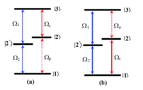
Figure 1: (a) Low-level probing scheme for two two-photon transitions atom-field system. (b) Up-level probing scheme for two two-photon transitions atom-field system.

The elements of the density matrix can be obtained directly from the master equation. It is known that for loop-transition, the relative of the fields plays important role in the result. The complex Rabi frequencies are defined as $\Omega_{c}=\Omega_{c}^{0}e^{i\phi_{c}},\Omega_{p}=\Omega_{p}^{0}e^{i\phi_{p}},\Omega_{1}=\Omega_{1}^{0}e^{i\phi_{1}},\Omega_{2}=\Omega_{2}^{0}e^{i\phi_{2}}$, where $\Omega_{j}^{0}$($j=p,c,1,2$) are strength of the Rabi frequencies.. In order to see the relative phase, we make the transformation as $\rho_{32}=\sigma_{32}e^{i\phi_{c}},\rho_{32^{{}^{\prime}}}=\sigma_{32^{{}^{\prime}}}e^{i\phi_{1}},\rho_{21}=\sigma_{21}e^{i\phi_{p}},\rho_{2^{{}^{\prime}}1}=\sigma_{2^{{}^{\prime}}1}e^{i\phi_{2}},\rho_{31}=\sigma_{31}e^{i(\phi_{1}+\phi_{2})},\rho_{22^{{}^{\prime}}}=\sigma_{22^{{}^{\prime}}}e^{i(\phi_{1}-\phi_{c})}$ and $\rho_{jj}=\sigma_{jj}$ $(j=1,2,2^{{}^{\prime}},3)$. After the transformation the motion of the elements are as following

$$\dot{\sigma}_{33} = -(\gamma_{1}+\gamma_{c})\sigma_{33}-i\Omega_{c}^{0}\sigma_{32}-i\Omega_{1}^{0}\rho_{32^{{}^{\prime}}}+i\Omega_{c}^{0}\sigma_{23}$$

$$+i\Omega_{1}^{0}\sigma_{2^{{}^{\prime}}3}$$

$$\dot{\sigma}_{22} = \gamma_{c}\sigma_{33}-\gamma_{p}\sigma_{22}+i\Omega_{c}^{0}\sigma_{32}-i\Omega_{p}^{0}\sigma_{21}-i\Omega_{c}^{0}\sigma_{23}$$

$$+i\Omega_{p}^{0}\sigma_{12}$$

$$\dot{\sigma}_{2^{{}^{\prime}}2^{{}^{\prime}}} = \gamma_{1}\sigma_{33}-\gamma_{2}\sigma_{2^{{}^{\prime}}2^{{}^{\prime}}}+i\Omega_{1}^{0}\sigma_{32^{{}^{\prime}}}-i\Omega_{2}^{0}\sigma_{2^{{}^{\prime}}1}-i\Omega_{1}^{0}\sigma_{2^{\prime}3}$$

$$+i\Omega_{2}^{0}\sigma_{12^{{}^{\prime}}}$$

$$\dot{\sigma}_{32} = -\Gamma_{32}\sigma_{32}-i\Omega_{c}^{0}(\sigma_{33}-\sigma_{22})-i\Omega_{p}^{0}e^{-i\phi}\sigma_{31}$$

$$+i\Omega_{1}^{0}\sigma_{2^{{}^{\prime}}2}$$

$$\dot{\sigma}_{32^{{}^{\prime}}} = -\Gamma_{32^{{}^{\prime}}}\sigma_{32^{{}^{\prime}}}-i\Omega_{1}^{0}(\sigma_{33}-\sigma_{2^{{}^{\prime}}2^{{}^{\prime}}})-i\Omega_{2}^{0}\sigma_{31}+i\Omega_{c}^{0}\sigma_{22^{{}^{\prime}}}$$

$$+i\Omega_{p}^{0}\sigma_{12}$$

$$\dot{\sigma}_{31} = -\Gamma_{31}\sigma_{31}-i\Omega_{p}^{0}e^{-i\phi}\sigma_{32}-i\Omega_{2}^{0}\sigma_{32^{{}^{\prime}}}+i\Omega_{c}^{0}e^{-i\phi}\sigma_{21}$$

$$+i\Omega_{1}^{0}\sigma_{2^{{}^{\prime}}1}$$

$$\dot{\sigma}_{22^{{}^{\prime}}} = -\Gamma_{22^{{}^{\prime}}}\sigma_{22^{{}^{\prime}}}+i\Omega_{c}^{0}\sigma_{32^{{}^{\prime}}}-i\Omega_{2}^{0}e^{-i\phi}\sigma_{21}-i\Omega_{1}^{0}\sigma_{23}$$

$$+i\Omega_{p}^{0}e^{-i\phi}\sigma_{12^{{}^{\prime}}}$$

$$\dot{\sigma}_{21} = -\Gamma_{21}\sigma_{21}-i\Omega_{p}^{0}(\sigma_{22}-\sigma_{11})+i\Omega_{c}^{0}e^{i\phi}\sigma_{31}$$

$$-i\Omega_{2}^{0}e^{i\phi}\sigma_{22^{{}^{\prime}}}$$

$$\dot{\sigma}_{2^{{}^{\prime}}1} = -\Gamma_{2^{{}^{\prime}}1}\sigma_{2^{\prime}1}-i\Omega_{2}^{0}(\sigma_{2^{{}^{\prime}}2^{{}^{\prime}}}-\sigma_{11})+i\Omega_{1}^{0}\sigma_{31}$$

$$-i\Omega_{p}^{0}e^{-i\phi}\sigma_{2^{{}^{\prime}}2}$$

where we have used the closed relation of the population $1=\rho_{11}+\rho_{22}+\rho_{2^{{}^{\prime}}2^{{}^{\prime}}}+\rho_{33}$, and $\rho_{jk}=\rho_{kj}^{*},k\neq j$ to obtain other elements with unlisted equations. We also defined $\gamma_{2^{{}^{\prime}}3}=\gamma_{1},\gamma_{23}=\gamma_{c},\gamma_{12^{{}^{\prime}}}=\gamma_{2},\gamma_{12}=\gamma_{p}$, and the related effective decay rates are $\Gamma_{32}=\frac{1}{2}(\gamma_{1}+\gamma_{c}+\gamma_{p})+i\Delta_{c}$, $\Gamma_{32^{{}^{\prime}}}=\frac{1}{2}(\gamma_{1}+\gamma_{c}+\gamma_{2})+i\Delta_{1}$, $\Gamma_{31}=\frac{1}{2}(\gamma_{1}+\gamma_{c})+i(\Delta_{p}+\Delta_{c})$, $\Gamma_{22^{{}^{\prime}}}=\frac{1}{2}(\gamma_{2}+\gamma_{p})+i(\Delta_{p}-\Delta_{2})$ and $\Gamma_{21}=\frac{1}{2}\gamma_{p}+i\Delta_{p},\Gamma_{2^{{}^{\prime}}1}=\frac{1}{2}\gamma_{2}+i\Delta_{2}$. $\phi=\phi_{1}+\phi_{2}-\phi_{c}-\phi_{p}$ is the relative phase of the applied fields. From the definition above the phase $\phi$ can also be understood as the relative phase between the two two-photon transitions $|1\rangle\leftrightarrow|2\rangle\leftrightarrow|3\rangle$ and $|1\rangle\leftrightarrow|2^{{}^{\prime}}\rangle\leftrightarrow|3\rangle$. As will shown below the relative phase plays a crucial role in the gain spectra.

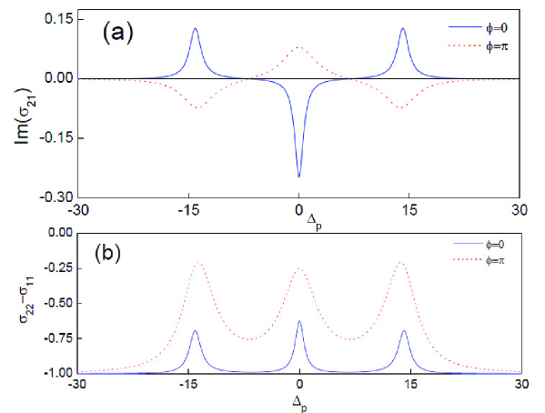
Figure 2: (a) Variation of Im($\sigma_{21}$) with probe detuning $\Delta_{p}$ for $\phi=0$ (solid line) and $\phi=\pi$ (dotted line) for $\Omega_{c}^{0}$ $=10$, $\Omega_{p}^{0}$ $=0.05$, $\Delta_{c}=\Delta_{1}=0$, $\Omega_{1}^{0}=10$ and $\Omega_{2}^{0}=1$. (c) Population difference $\sigma_{22}-\sigma_{11}$ vesus probe detuning $\Delta_{p}$ corresponding to gain in (a).

Steady state solution of the master equation can be obtained by setting $\dot{\sigma}_{ij}=0$. Absorption behavior of the weak probe field $\Omega_{p}$ is described by Im($\sigma_{21}$). When Im($\sigma_{21}$)$<0$, it symbols gain behavior. In our calculation we set $\gamma_{j}=\gamma=1$ ($j=p,c,1,2$), and scale all the $\Omega_{j}^{0}$ and detunings $\Delta_{j}$ ($j=p,c,1,2$) in units of $\gamma$. We choose the probe field to be weak and real. The main results are shown in Fig. 2.

Phase-dependent gain and corresponding population difference $\sigma_{22}-\sigma_{11}$ vesus probe detuning $\Delta_{p}$ is shown in Fig. 2. Im($\sigma_{21}$) vesus probe detuning $\Delta_{p}$ for $\phi=0$ (solid line) and $\phi=\pi$ (dotted line) is plotted in Fig. 2(a). Other parameters are chosen as $\Omega_{c}^{0}$ $=10$, $\Omega_{p}^{0}=0.05$, $\Delta_{c}=\Delta_{1}=0$, $\Omega_{1}^{0}=10$ and $\Omega_{2}^{0}=1$. Corresponding population difference $\sigma_{22}-\sigma_{11}$ vesus probe detuning $\Delta_{p}$ in (a) is shown in Fig. 2(b). Seen from Fig. 2(a), it is clear that when the relative phase $\phi$ changes from $0$ to $\pi$, the probe field experiences different gain shapes. Gain and absorption zones exchange. The most remarkable change lies in the fact that the gain zones has increased from a single zone near resonant point $\Delta_{p}=0$ to two separate frequency zones localling around $\Delta_{p}=\pm 15.9$. This means that the number of gain zones are controlled by the relative phase of the applied fields. And seen fro Fig. 2(b), population difference $\sigma_{22}-\sigma_{11}<0$ always holds, which suggests that population inversion is impossible during the interaction. So the gain behavior does not come from population inversion between levels $|2\rangle$ and $|1\rangle$.

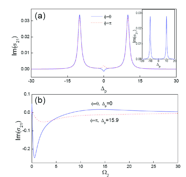
Figure 3: (a) Variation of Im($\sigma_{21}$) with probe detuning $\Delta_{p}$ for $\phi=0$ (solid line) and $\phi=\pi$ (dotted line) for $\Omega_{c}^{0}$ $=10$, $\Omega_{p}^{0}$ $=0.05$, $\Delta_{c}=\Delta_{1}=0$, $\Omega_{1}^{0}=0.1$ and $\Omega_{2}^{0}=0.1$. The inner graph in Fig. 3(a) is the absorption spectrum vesus $\Delta_{p}$ for three-level cascade driving without the transitions coupled by the fields $\Omega_{1}$ and $\Omega_{2}$. (b) Probe gain versus $\Omega_{2}^{0}$ for $\phi=0,\Delta_{p}=0$ (solid line) and $\phi=\pi$, $\Delta_{p}=15.9$ (dotted line). The other parameters are the same as those in Fig. 2(a).

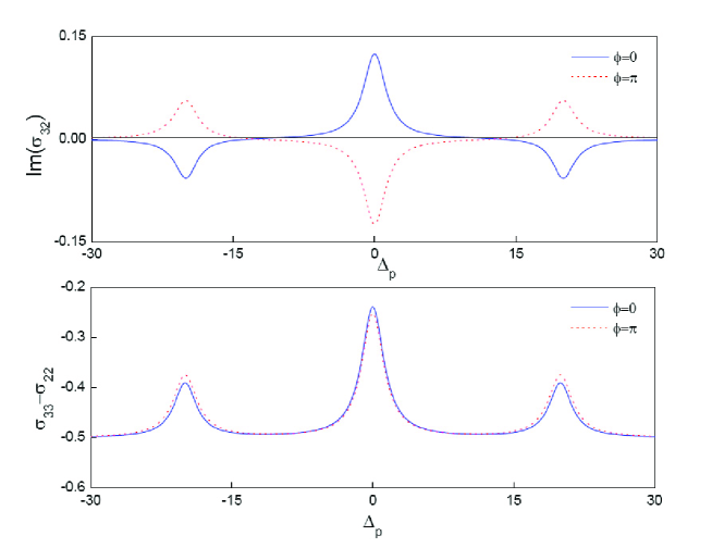
Figure 4: (a) Variation of Im($\sigma_{32}$) with probe detuning $\Delta_{p}$ for $\phi=0$ (solid line) and $\phi=\pi$ (dotted line) for $\Omega_{c}^{0}$ $=10$, $\Omega_{p}^{0}$ $=0.05$, $\Delta_{c}=\Delta_{1}=0$, $\Omega_{1}^{0}=10$ and $\Omega_{2}^{0}=1$ (b) Population difference $\sigma_{33}-\sigma_{22}$ vesus probe detuning $\Delta_{p}$ corresponding to gain in (a).

Fig. 3(a) shows the case with small driving of one two-photon transition, i.e., $\Omega_{1}^{0}$ $=\Omega_{2}^{0}$ $=0.1$ for $\phi=0$ (solid lines) and $\phi=\pi$ (dotted lines) , and the other parameters are the same as those in Fig. 2(a). Two feathers are presented. One is that the probe absorption domains with two remarkable absorption peaks. The other is that when the phase changes from $0$ to $\pi$, the probe gain around the resonant point goes into the probe absorption while the dominated absorption keeps unchanged. In order to see the effects of the two two-photon transitions, we plot the probe absorption for the case of one two-photon transition $|1\rangle\leftrightarrow|2\rangle\leftrightarrow|3\rangle$ with the same parameters. The inner graph in Fig. 3(a) is the absorption spectrum vesus $\Delta_{p}$ for three-level cascade driving without the transitions coupled by the fields $\Omega_{1}$ and $\Omega_{2}$. The results show that electromagnetically induced transparency can be obtained and no phase dependence and no gain are found for single two-photon transition. Thus it is the two two-photon transitions is the origin of the probe gain and the phase dependence. In Fig. 3(b) the probe absorption Im($\sigma_{21}$) vesus $\Omega_{2}^{0}$, the amplitude of $\Omega_{2}$ is also plotted for $\phi=0,\Delta_{p}=0$ (solid line) and $\phi=\pi$, $\Delta_{p}=15.9$ (dotted line). The other parameters are the same as those in Fig. 2(a). It is easy to see that the parameters we choose in Fig. 2(a) are optimal for gain behavior.

Figure 5: (a) Variation of Im($\sigma_{32}$) with probe detuning $\Delta_{p}$ for $\phi=0$ (solid line) and $\phi=\pi$ (dotted line) for $\Omega_{c}^{0}$ $=10$, $\Omega_{p}^{0}$ $=0.05$, $\Delta_{c}=\Delta_{1}=0$, $\Omega_{1}^{0}=0.1$ and $\Omega_{2}^{0}=0.1$. The inner graph in Fig. 5(a) is the absorption spectrum vesus $\Delta_{p}$ for three-level cascade driving without the transitions coupled by the fields $\Omega_{1}$ and $\Omega_{2}$. (b) Probe gain versus $\Omega_{2}^{0}$ for $\phi=0,\Delta_{p}=20.2$ (solid line) and $\phi=\pi$, $\Delta_{p}=0$ (dotted line). The other parameters are the same as those in Fig. 4(a).

When we exchange the probe field $\Omega_{p}$ and the driving field $\Omega_{c}$ with coupling scheme shown in Fig. $1$(b), gain without inversion can also be obtained. We call this case up-level probing. The results are presented in Fig. 4 and Fig. 5 with similar parameters as those in Fig. 2 and Fig. 3. It is clear that gain without inversion also exhibits in such a system and the phase dependence of the gain on relative phase $\phi$ is presented as well. There are two differences between the low level probing and the up level probing case. One is that the number of gain zone is different with the same phase. For specific, when $\phi=0$, the low-level coupling has single gain without inversion zone at $\Delta_{p}=0$ while the up-level coupling has two gain without inversion zones at $\Delta_{p}=\pm 20.2$; when $\phi=\pi$, the low-level coupling has two gain without inversion zones at $\Delta_{p}=\pm 15.9$ while the up-level coupling has only one gain without inversion zones at $\Delta_{p}=0$. The other feature is that no gain is presented when the two-photon transition $|1\rangle\leftrightarrow|2^{{}^{\prime}}\rangle\leftrightarrow|3\rangle$ is small when the phase changes from $0$ to $\pi$ and the phase just makes the shift of the absorption a little. In a word the absorption spectra act like the probe absorption for the case of one two-photon transition $|1\rangle\leftrightarrow|2\rangle\leftrightarrow|3\rangle$ with the same parameters except the phase influence. In Fig. 5(b) the dependence of probe gain on $\Omega_{2}^{0}$ is also presented. From this, one can see that the optimal parameters are used in Fig. 4(a).

To under stand the above results, we can simply use the steady state expression of two terms as following

$$\mathop{\rm Im}(\sigma_{21}) = \frac{1}{D}\mathop{\rm Im}[(\frac{\gamma_{p}}{2}-i\Delta_{p})(i\Omega_{c}^{0}\sigma_{31}-i\Omega_{2}^{0}\sigma_{22^{{}^{\prime}}})e^{i\phi}]$$ (6)

$$-\frac{\frac{1}{2}\Omega_{p}^{0}\gamma_{p}(\sigma_{22}-\sigma_{11})}{\frac{1}{4}\gamma_{p}^{2}+\Delta_{p}^{2}}$$

$$\mathop{\rm Im}(\sigma_{32}) = \frac{1}{D}\mathop{\rm Im}[(\frac{\gamma_{c}}{2}-i\Delta_{c})(-i\Omega_{p}^{0}e^{-i\phi}\sigma_{31}+i\Omega_{1}^{0}\sigma_{2^{{}^{\prime}}2})]$$ (7)

$$-\frac{\frac{1}{2}\Omega_{c}^{0}\gamma_{c}(\sigma_{33}-\sigma_{22})}{\frac{1}{4}\gamma_{c}^{2}+\Delta_{c}^{2}}$$

where $D=\frac{1}{4}\gamma_{p}^{2}+\Delta_{p}^{2}$ . From eq. (6), it is easy to see that when no population inversion happens, i.e., $(\sigma_{22}-\sigma_{11})<0$, the first term is always positive. So when gain occurs (Im$(\sigma_{21})<0$), the second term contributes. Similar results also hold for up-level probing case just by make the replace of $\sigma_{21}$ by $\sigma_{32}$ and exchange the field $\Omega_{c}$ and $\Omega_{p}$. Due to pure absorption and no phase-dependent behavior of three-level cascade driving $|1\rangle\leftrightarrow|2\rangle\leftrightarrow|3\rangle$ by $\Omega_{c}$ and $\Omega_{p}$, we can conclude that it is the two-photon transition $|1\rangle\leftrightarrow|2^{{}^{\prime}}\rangle\leftrightarrow|3\rangle$ driving by $\Omega_{1}$ and $\Omega_{2}$ that induces the gain without inversion and the two two-photon transitions $|1\rangle\leftrightarrow|2(2^{{}^{\prime}})\rangle\leftrightarrow|3\rangle$ loop structure induces the phase dependence of the gain behavior.

In conclusion, gain without inversion in a four level loop-transition atomic system has been investigated. The main results are two features: (i) Gain without inversion is exhibited by varing the amplitude of coupled fields. (ii) Gain without inversion displays a phase dependence on the relative phase between the fields applied on the two two-photon transitions. As the phase changes from 0 to $\pi$, gain and absorption zones exchange. Population inversionless holds for all the case. Gain without inversion and phase-dependence are attributed to interference induced by such a loop-transition structure.

Acknowledgments This work is supported by the Scientific Research Plan of the Provincial Education Department in Hubei (Grant No. Q20101304) and NSFC under Grant No. 11147153.

References

(1) G. S. Agarwal, Opt.Commun. 80, 37 (1990).
(2) Y. Zhu, Q. Wu and T. M. Mossberg, Phys. Rev. Lett. 65, 1200 (1990).
(3) A. Lezama, Y. Zhu and T. M. Mossberg, Phys. Rev. A 41, 1576 (1990).
(4) G. Khitrova, J. Fi. Valley and H. M. Gibbs, Phys. Rev. Lett. 60, 1126 (1988).
(5) M. O. Scully S. Y. Zhu, and A. Gavrielides, Phys. Rev. Lett. 62, 2813 (1989).
(6) Gain 2010
(7) G. S. Agarwal, S. Ravi and J. Cooper, Phys. Rev. A 41,
4721 (1990).
(8) S. E. Harris, Phys. Rev. Lett. 62, 1033 (1989).
(9) A. Imamoglu, Phys. Rev. A 40, 2835 (1989).
(10) Y. S. Zhu, Phys. Rev. A 42, 5537 (1990).
(11) Y. S. Zhu and E. E. Fill, Phys. Rev. A 42, 5684 (1990).
(12) L. Nu and P. R. Berman, Phys. Rev. A 44, 5965 (1991).
(13) M. D. Frogley, J. F. Dynes, M. Beck, J. Faist and C. C.
Phillips, Nature materials 5, 175 (2006).
(14) D. Kosachiov, B. Matisov and Y. Rozhdestvensky, Opt.Commun.
85, 209 (1991).
(15) B. P. Hou, S. J. Wang, W. L. Yu and W. L. Sun, J. Phys. B 38, 1419 (2005).
(16) B. H. Li, V. A. Sautenkov, Y. V. Rostovtsev, G. R. Welch, P.
R. Hemmer and M. O. Scully, Phys. Rev. A 80, 023820 (2009).
(17) D. V. Kosachiov, B. G. Matisov and Y. V. Rozhdestvensky, J.
Phys. B 25, 2473 (1992).
(18) E. Paspalakis and P. L. Knight, Phys. Rev. Lett. 81, 293
(1998).
(19) F. Ghafoor, S.Y. Zhu and M. S. Zubairy, Phys. Rev. A 62,
013811 2000.
(20) X. X. Li, X. M. Hu, W. X. Shi, Q. Xu, H. J. Guo and J. Y. Li,
Chin. Phys. Lett. 23, 340 (2006).
(21) X. M. Hu, W. X. Shi, Q. Xu, H. J. Guo, J. Y. Li and X. X. Li,
Phys. Lett. A 352, 543 (2006).
(22) Phys. Rev. Lett. 105, 073601 (2010).
(23) M. O. Scully and M. S. Zubairy, Quantum Optics
(Cambridge University Press 1997.