Coordinated Multicast Beamforming in Multicell Networks

Abstract

We study physical layer multicasting in multicell networks where each base station, equipped with multiple antennas, transmits a common message using a single beamformer to multiple users in the same cell. We investigate two coordinated beamforming designs: the quality-of-service (QoS) beamforming and the max-min SINR (signal-to-interference-plus-noise ratio) beamforming. The goal of the QoS beamforming is to minimize the total power consumption while guaranteeing that received SINR at each user is above a predetermined threshold. We present a necessary condition for the optimization problem to be feasible. Then, based on the decomposition theory, we propose a novel decentralized algorithm to implement the coordinated beamforming with limited information sharing among different base stations. The algorithm is guaranteed to converge and in most cases it converges to the optimal solution. The max-min SINR (MMS) beamforming is to maximize the minimum received SINR among all users under per-base station power constraints. We show that the MMS problem and a weighted peak-power minimization (WPPM) problem are inverse problems. Based on this inversion relationship, we then propose an efficient algorithm to solve the MMS problem in an approximate manner. Simulation results demonstrate significant advantages of the proposed multicast beamforming algorithms over conventional multicasting schemes.

I Introduction

With the rapid development of wireless communication technology, various kinds of traditional data service, such as media streaming, cell broadcasting and mobile TV, have been implemented in wireless networks nowadays. As a result, wireless multicasting becomes a central feature of the next generation cellular networks. Physical layer multicasting with beamforming is a promising solution enabled by exploiting channel state information (CSI) at the transmitter over the traditional isotropic broadcasting. The problem of multicast beamforming for quality-of-service (QoS) guarantee and for max-min fairness was firstly considered in [1]. The similar problem of multicasting to multiple cochannel groups was then investigated in [2]. The core problem of multicast beamforming is essentially NP-hard [1]. Some other issues such as outage analysis and capacity limits were studied in [3], [4]. So far multicast beamforming has been included in the UMTS-LTE / EMBMS draft for next-generation cellular wireless services [5], [6].

In conventional wireless systems, signal processing is performed on a per-cell basis. The intercell interference is treated as background noise and minimized by applying a predesigned frequency reuse pattern such that the adjacent cells use different frequency bands. Due to the fast growing demand for high-rate wireless multimedia applications, many beyond-3G wireless technologies such as 3GPP-LTE and WiMAX have relaxed the constraint on the frequency reuse such that the total frequency band is available for reuse by all cells in the same cluster. However, this will cause the whole system limited by the intercell interference. Consequently, cooperative signal processing across the different base stations has been identified as a key technique to mitigate intercell interference in the next-generation wireless systems.

The goal of this paper is to investigate multicast beamforming for cooperative multicell networks. The base stations cooperate with each other and design their transmit beamformers in a coordinated manner. In general, there are two cooperation scenarios in multicell networks. In the first scenario, different base stations are fully cooperative and act as “networked MIMO (multiple-input multiple-output)” (e.g., [7],[8]). Namely, they coordinate in the signal level, i.e., data information intended for different users in different cells is shared among the base stations. Clearly, networked MIMO needs tremendous amount of information exchange overhead. In contrast, in the second scenario, the base stations are only required to coordinate at the beamforming level which needs rather small information sharing (e.g., [9]). In this paper, we focus on the latter case by only allowing beamforming level coordination.

We first formulate the problem of multicell multicast beamforming as sum power minimization subject to the constraint that the received signal-to-interference-plus-noise ratio (SINR) of each user is above a threshold. This problem is referred to as QoS problem. It is known that the QoS problem in single-cell scenario is always feasible. However, this is not so in multicell networks due to the intercell interference, especially when the channel condition is bad or the SINR target is very stringent. We first present a necessary condition on the optimization problem to be feasible. Then we propose a novel distributed algorithm to solve the multicell multicast cooperative beamforming design. More specifically, based on the decomposition theory [10], we introduce a set of interference constraint parameters and decompose the original problem into several parallel sub-problems. Since the sub-problems are nonconvex and NP-hard, each base station then applies the semidefinite relaxation and independently solves its own sub-problem. The interference parameters are updated based on a master problem. Simulation results show that the algorithm converges in only several iterations.

In view of the user fairness issue, we also consider the multicell multiast beamforming design with the goal of maximizing the minimum SINR (MMS) among all users under individual power constraints. This is called MMS problem. By linking the MMS problem with a weighted peak power minimization (WPPM) problem, we propose an efficient algorithm to find the near-optimal solution. Previously, the authors in [11] [12] also studied the multicell multicast beamforming problem with the objective to maximize the minimum SINR but subject to a total sum power constraint across all base stations. Hence, the problem considered in [11] [12] is very similar to the multicast beamforming problem in single-cell multi-group systems as in [2]. Authors in [13] also considered the similar problem under per-base-station power constraint but allowed data sharing among base stations, which is similar to the “network MIMO” and requires a large amount of information exchange overhead. Thus, our beamforming design for max-min fairness is more practical as we consider individual peak power constraint on each base station and only allow coordination in the beamforming level.

The rest of the paper is organized as follows. In Section II, the system model for multicell multicasting is presented. Section III considers the beamformer design in the QoS problem and develops a novel decentralized coordinated beamforming algorithm. In Section IV, we consider the max-min SINR beamforming problem under individual base station power constraints. Section V provides simulation results. Concluding remarks are made in Section VI.

Notations: $\mathds{R}$ and $\mathds{C}$ denote the real and complex spaces. The identity matrix is denoted as I and the all-one vector is denoted as ${\bf 1}$. For a square matrix S, $\textsl{{S}}\succeq 0$ means that S is positive semi-definite. $[{\bf H}]_{i,j}$ denotes its element in the $i$th row and $j$th column. $(\cdot)^{\textsl{T}}$, $(\cdot)^{\textsl{H}}$, $(\cdot)^{\dagger}$ and $\mbox{Tr}\{\cdot\}$ stand for transpose, Hermitian transpose, Moore Penrose pseudoinverse and the trace respectively. $|x|$ denotes the absolute value of the scalar $x$ and $\|\bf{x}\|$ denotes the Euclidean norm of the vector $\bf{x}$.

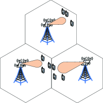
Figure 1: Multicell multicast network.

II System Model

Consider a multicell multicast network comprising $N$ cells and $K$ mobile users per cell as shown in Fig. 1. The base station in each cell is equipped with $N_{t}$ antennas and every mobile user has a single antenna. Let ${\bf{h}}_{i,j,k}^{H}$ denote the frequency-flat quasi-static $1\times N_{t}$ complex channel vector from the base station in the $i$th cell to the $k$th user in the $j$th cell, and $\textbf{w}_{i}$ denote the $N_{t}\times 1$ multicast beamforming vector applied to the base station in the $i$th cell. We define the complex scalar $s_{i}$ as the multicast information symbol for the users in the $i$th cell. The discrete-time baseband signal received by the $k$th user in the $i$th cell is given by

$${y_{i,k}}={{\bf h}_{i,i,k}^{\emph{H}}}{{\bf w}_{i}}{s_{i}}+\sum^{N}_{j\neq i}{{\bf h}_{j,i,k}^{\emph{H}}}{{\bf w}_{j}}{s_{j}}+z_{i,k},$$ (1)

where $z_{i,k}$ is the additive white circularly symmetric Gaussian complex noise with variance $\sigma_{i,k}^{2}/2$ on each of its real and imaginary components. In (1), the second term is the intercell interference.

Based on the received signal model in (1), the performance of each user can be characterized by the output SINR, defined as

$${\mbox{SINR}_{i,k}}=\frac{{|{\bf h}_{i,i,k}^{\emph{H}}{\bf w}_{i}|}^{2}}{\sum^{N}_{j\neq i}{|{\bf h}_{j,i,k}^{\emph{H}}{\bf w}_{j}|}^{2}+\sigma_{i,k}^{2}}.$$ (2)

Notice that each user in the considered multicell multicast network only suffers from the intercell interference, which is different from multicell unicast systems where both inter-cell interference and intra-cell interference exist.

In practical scenarios, the channels from a base station to different users, which may or may not belong to a same cell, can be correlated, especially when these users are in close proximity to each other. For the users belonging to the same cell, we call the correlation between ${\bf h}_{i,j,k}^{H}$ and ${\bf h}_{i,j,k^{\prime}}^{H}$ for $k\neq k^{\prime}$ as the intracell-user channel correlation. For the users from different cells, we call the correlation between ${\bf h}_{i,j,k}^{H}$ and ${\bf h}_{i,j^{\prime},l}^{H}$ for $j\neq j^{\prime}$ as the intercell-user channel correlation.

III QoS Beamforming

The coordinated QoS beamforming design is to minimize the total energy consumption of the system while maintaining a target SINR for all users by properly designing the beamformers at each base station. This is formulated as:

$${\bf P}({\bm{\gamma}}): \min\limits_{\{{\bf w}_{i}\}_{i=1}^{N}} \sum\limits_{i=1}^{N}\|{\bf w}_{i}\|^{2}$$ (3)

s.t. $$\frac{|{\bf h}_{i,i,k}^{\emph{H}}{\bf w}_{i}|^{2}}{\sum\limits_{j\neq i}^{N}|{\bf h}_{j,i,k}^{\emph{H}}{\bf w}_{j}|^{2}+\sigma^{2}_{i,k}}\geq\gamma_{i},\forall i,k$$ (4)

where ${\bm{\gamma}}=[\gamma_{1},\gamma_{2},...,\gamma_{N}]^{T}$ is the target SINR vector with each element $\gamma_{i}$ being the target SINR value to be achieved by the users in the $i$th cell. Since the base station transmits a common information in a multicast manner, the information rate for the users within one cell is the same, and hence we set a common SINR target for all the users in the same cell.

III-A Feasibility analysis

Due to the SINR constraints, the QoS problem in (3) is not always feasible, which is similar to the multiuser unicast scenario [14]. In order to verify its feasibility, we need to show whether there exists a set of beamformers $\{{\bf w}_{i}\}_{i=1}^{N}$ for a given ${\bm{\gamma}}$ such that

$$\min_{k}~{}\mbox{SINR}_{i,k}\geq\gamma_{i},\forall i\in\{1,2,...,N\}$$ (5)

For simplicity, the SINR targets for different cells are assumed to be the same. Then the above condition boils down to the following

$$\min_{i,k}~{}\mbox{SINR}_{i,k}\geq\gamma$$ (6)

For the $k$th user in each cell, we combine their channel vectors as follows

$${\bf H}_{k}=\begin{bmatrix}{\bf h}_{1,1,k}^{H}&{\bf h}_{2,1,k}^{H}&\cdots&{\bf h}_{N,1,k}^{H}\\ {\bf h}_{1,2,k}^{H}&{\bf h}_{2,2,k}^{H}&\cdots&{\bf h}_{N,2,k}^{H}\\ \vdots&\cdots&~{}&~{}\\ {\bf h}_{1,N,k}^{H}&{\bf h}_{2,N,k}^{H}&\cdots&{\bf h}_{N,N,k}^{H}\end{bmatrix},~{}k=1,2,...,K$$ (7)

where each ${\bf H}_{k}$ is an $N\times(N\times N_{t})$ matrix. The following lemma provides a necessary condition for the QoS problem to be feasible.

Lemma 1: Given the SINR target vector ${\bm{\gamma}=\gamma\cdot{\bf 1}}$, if the problem (3) is feasible, then the SINR target $\gamma$ should satisfy the following condition

$$\gamma\leq\min\left\{\frac{\mbox{rank}({\bf H}_{1})}{{\emph{N}}-\mbox{rank}({\bf H}_{1})},\cdots,\frac{\mbox{rank}({\bf H}_{K})}{{\emph{N}}-\mbox{rank}({\bf H}_{K})}\right\}$$ (8)

Proof:

Please refer to Appendix A. ∎

From Lemma 1, we can see that the intercell-user channel correlation has a negative impact on its feasibility. More specifically, if some of the rows in ${\bf H}_{k}$, say the $i$th row and $i^{\prime}$th row for $i\neq i^{\prime}$, are correlated, which means that the channels between the $k$th user in the $i$th cell and the $k$th user in the $i^{\prime}$th cell are correlated, then the rank of ${\bf H}_{k}$ could be less than $N$ and as a result, the SINR threshold $\gamma$ will have a finite upper bound. On the other hand, if the channels of users in different cells are independent, we have that the matrix ${\bf H}_{k}$ is full rank with probability one, then the corresponding upper bound is infinite, which means no constraint on $\gamma$. Since the problem (3) is NP-hard [2], determining its feasibility is not an easy job. The lemma gives a necessary condition from the perspective of channel correlation. In the following, we only consider the problem (3) when it is feasible.

III-B Decentralized coordinated beamforming

A desired feature of coordinated beamforming in multicell networks is that the base station at each cell can implement its beamforming design locally [17], [18]. This is due to the constraint in practical systems that the backhaul channel has limited capacity. In this subsection, we propose a decentralized scheme for implementing the multicell multicast QoS beamforming. It is assumed that each base station in the network only has the channel knowledge of the mobile users within its own cell.

The distributed algorithm to problem ${\bf P}(\bm{\gamma})$ can not be easily obtained primarily because all the beamformers are coupled together in the constraint (4). According to the decomposition theory [10] and inspired by [18], we introduce a set of slack variables $\Gamma_{i,j,k}$ denoting the constraint of the interference from the $i$th base station to the $k$th user in the $j$th cell. Then the problem $\bf P(\bm{\gamma})$ can be reformulated as

$${\bf P}(\bm{\gamma},{\bf\Gamma}): \min\limits_{\{{\bf w}_{i}\}_{i=1}^{N}} \sum_{i=1}^{N}{\|{\bf w}_{i}\|}^{2}$$ (9)

s.t. $$\frac{{|{\bf h}_{i,i,k}^{\emph{H}}{\bf w}_{i}|}^{2}}{\sum\limits_{j\neq i}^{N}\Gamma_{j,i,k}+\sigma^{2}_{i,k}}\geq\gamma_{i},\forall i,k$$ (10)

$${|{\bf h}_{i,j,k}^{\emph{H}}{\bf w}_{i}|}^{2}\leq\Gamma_{i,j,k},\forall i,j\neq i,k$$ (11)

Here, the real-valued vector ${\bf\Gamma}$ is defined as follows

$${\bf\Gamma}=(\Gamma_{1,2,1},...,\Gamma_{1,2,K},...,\Gamma_{N,N-1,K})^{T}\in\mathds{R}^{\left(N\left(N-1\right)K\right)\times 1}$$ (12)

The introduction of ${\bf\Gamma}$ is similar to the concept of interference temperature (IT) in cognitive radios and hence we refer to it as IT vector. It is now observed that the constraints in (10) are all decoupled. Unlike [18], our problem is still nonconvex and NP-hard. We cannot solve it by exploiting its dual problem since the strong duality does not hold. In the following we take the semidefinite relaxation (SDR) approach, the optimality of which shall be discussed later in this section. Introducing new variables $\{{\bf W}_{i}={\bf w}_{i}{\bf w}^{\emph{H}}_{i}\}_{i=1}^{N}$, the relaxed problem of ${\bf P}({\bm{\gamma}},{\bm{\Gamma}})$ becomes:

$${\bf P}_{1}(\bm{\gamma},{\bf\Gamma}):\min\limits_{\{{\bf W}_{i}\}_{i=1}^{N}}\sum\limits_{i=1}^{N}\mbox{Tr}\{{\bf W}_{i}\}~{}~{}~{}~{}~{}~{}~{}~{}~{}~{}~{}~{}~{}~{}~{}~{}~{}~{}~{}~{}~{}~{}~{}~{}~{}~{}~{}~{}~{}~{}$$ (13)

$$~{}\mbox{s.t.}~{}~{}{\mbox{Tr}\{{\bf H}_{i,i,k}{\bf W}_{i}\}}\geq\gamma_{i}{{\bf e}_{i,i,k}^{T}{\bf\Gamma}+\gamma_{i}\sigma^{2}_{i,k}},\forall i,k$$ (14)

$$\mbox{Tr}\{{\bf H}_{i,j,k}{\bf W}_{i}\}\leq{\bf e}_{i,j,k}^{T}{\bf\Gamma},\forall i,j\neq i,k~{}~{}~{}~{}~{}$$ (15)

$${\bf W}_{i}\succeq{\bf 0}~{}~{}~{}~{}~{}~{}~{}~{}~{}~{}~{}~{}~{}~{}~{}~{}~{}~{}~{}~{}~{}~{}~{}~{}~{}~{}~{}~{}~{}~{}~{}~{}~{}~{}~{}~{}~{}~{}$$ (16)

Here, for notation convenience we have introduced the $\left(N\left(N-1\right)K\right)\times 1$ direction vectors ${\bf e}_{i,j,k}$ and defined ${\bf H}_{i,j,k}\triangleq{\bf h}_{i,j,k}{\bf h}_{i,j,k}^{H}$.

For a pre-fixed IT vector $\bf\Gamma$, since the constraints have been decoupled, problem ${\bf P}_{1}(\bm{\gamma},{\bf\Gamma})$ can be decomposed into $N$ parallel subproblems. The $i$th subproblem is as follows

$${\bf P}^{\mbox{sub}}_{i}(\bm{\gamma},{\bf\Gamma}):~{}\min\limits_{{\bf W}_{i}}\mbox{Tr}\{{\bf W}_{i}\}~{}~{}~{}~{}~{}~{}~{}~{}~{}~{}~{}~{}~{}~{}~{}~{}~{}~{}~{}~{}~{}~{}~{}~{}~{}~{}~{}~{}~{}~{}~{}~{}~{}~{}~{}$$ (17)

$$\mbox{s.t.}~{}~{}{\mbox{Tr}\{{\bf H}_{i,i,k}{\bf W}_{i}\}}\geq\gamma_{i}{{\bf e}_{i,i,k}^{T}{\bf\Gamma}+\gamma_{i}\sigma^{2}_{i,k}},\forall k$$ (18)

$$\mbox{Tr}({\bf H}_{i,j,k}{\bf W}_{i})\leq{\bf e}_{i,j,k}^{T}{\bf\Gamma},\forall j\neq i,k~{}~{}~{}~{}~{}~{}$$ (19)

$${\bf W}_{i}\succeq{\bf 0}~{}~{}~{}~{}~{}~{}~{}~{}~{}~{}~{}~{}~{}~{}~{}~{}~{}~{}~{}~{}~{}~{}~{}~{}~{}~{}~{}~{}~{}~{}~{}~{}~{}~{}~{}~{}$$ (20)

It is easily observed that in each subproblem, the base station only needs the local channel state information. Specifically, the $i$th cell’s base station needs just the channel vectors ${\bf h}_{i,j,k}^{H},\forall j=1\cdots N,\forall k=1\cdots K$. Since it is also convex, the optimal solution can be obtained efficiently. Having solved the subproblems, we then define the master problem in charge of updating the IT vector ${\bf\Gamma}$

$${\bf P}^{\mbox{mas}}(\bm{\gamma}):~{}\min_{\bf\Gamma}~{}~{}P\left(\bm{\Gamma}\right)$$ (21)

where $P\left(\bm{\Gamma}\right)=\sum\limits_{i=1}^{N}P_{i}^{\star}({\bf\Gamma})$ with $P_{i}^{\star}({\bf\Gamma})$ being the optimal solution of problem ${\bf P}^{\mbox{sub}}_{i}(\bm{\gamma},{\bf\Gamma})$ for a given ${\bf\Gamma}$. This master problem can be solved iteratively using a subgradient projection method. Denote ${\bf g}\in\mathds{R}^{\left(N\left(N-1\right)K\right)\times 1}$ as the global subgradient of $P\left(\bm{\Gamma}\right)$ at ${\bm{\Gamma}}$. The following theorem suggests that $\bf g$ can be obtained from each base station.

$\textbf{Theorem 1}:$ The global subgradient $\bf g$ of $P\left(\bm{\Gamma}\right)$ in the master problem ${\bf P}^{\mbox{mas}}(\bm{\gamma})$ is given by

$${\bf g}=\sum_{i=1}^{N}{\bf g}_{i}$$ (22)

where ${\bf g}_{i}$ is the subgradient of $P_{i}^{\star}({\bf\Gamma})$.

Proof:

Please refer to Appendix B. ∎

According to Theorem 1, every base station first solves its own subproblem, gets the subgradient vector ${\bf g}_{i}$ and then broadcasts it to other cells. Upon receiving all the $N$ subgradient vectors ${\bf g}_{i}$’s, the base station in each cell will sum them up to get the subgradient ${\bf g}$ and update the IT vector $\bf\Gamma$ as below

$${\bf\Gamma}(n+1)=\left[{\bf\Gamma}(n)-\mu(n)\cdot\frac{{\bf g}(n)}{\|{\bf g}(n)\|}\right]^{+},$$ (23)

where $n$ denotes the iteration index and $\mu$ is the step size. Here, $[\cdot]^{+}$ denotes the projection onto the nonnegative orthant. Since the problem ${\bf P}_{1}(\bm{\gamma},{\bf\Gamma})$ is convex, this distributed algorithm is guaranteed to converge and converge exactly to the optimal solution of ${\bf P}_{1}(\bm{\gamma},{\bf\Gamma})$. Just like the steepest descent method, the choice of step size affects the convergence properties of the iterative algorithm, such as the speed and the accuracy. Here we just take the simple diminishing step, i.e., $\mu(n)=s/{\sqrt{n}}$, where $s>0$ is the initial step size.

When the algorithm converges, each base station can get its own beamformer from its resulting matrix ${\bf W}_{i}^{\star}$. We now discuss how to extract the beamformer vector ${\bf w}_{i}$ from each ${\bf W}_{i}^{\star}$ and its optimality. Since the original problem ${\bf P}(\bm{\gamma})$ is NP-hard, generally there is no guarantee that an algorithm for solving the relaxed SDP problem will give the desired rank-one solution. If the ${\bf W}_{i}^{\star}$ is rank-one, then the base station applies the eigen-value decompsotion (EVD) to ${\bf W}_{i}^{\star}$ as ${\bf W}_{i}^{\star}=\lambda_{i}^{\star}{\bf w}_{i}^{\star}{{\bf w}_{i}^{\star}}^{H}$ and takes ${\bf w}_{i}=\sqrt{\lambda_{i}^{\star}}{\bf w}_{i}^{\star}$ as the optimal beamformer. Otherwise, it first generates a set of candidate beamforming vectors $\{{\bf w}_{i}^{l}\}$ by randomization method. Specifically, one can perform EVD on ${\bf W}_{i}^{\star}$ to get ${\bf W}_{i}^{\star}={\bf U}_{i}{\bm{\Sigma}}_{i}{\bf U}_{i}^{H}$ and then generate the $l$th candidate vector ${\bf w}_{i}^{l}$ as ${\bf w}_{i}^{l}={\bf U}_{i}{\bm{\Sigma}}_{i}^{1/2}{\bf v}_{l}$, where ${\bf v}_{l}\sim\mathcal{CN}({\bf 0},\bf I)$. Then based on its own subproblem ${\bf P}^{\mbox{sub}}_{i}(\bm{\gamma},{\bf\Gamma})$, the base station needs to do scaling to get the beamforming vector. The scaling problem is formulated as below

$${\bf L}_{i}(\bm{\gamma},{\bf\Gamma}):~{}\min\limits_{\alpha_{i}}~{}~{}\alpha_{i}~{}~{}~{}~{}~{}~{}~{}~{}~{}~{}~{}~{}~{}~{}~{}~{}~{}~{}~{}~{}~{}~{}~{}~{}~{}~{}~{}~{}~{}~{}~{}~{}~{}~{}~{}~{}~{}~{}~{}~{}~{}~{}~{}$$ (24)

$$\mbox{s.t.}~{}~{}{\alpha_{i}|{\bf h}_{i,i,k}^{H}{\bf w}^{\prime}_{i}|^{2}}\geq\gamma_{i}{{\bf e}_{i,i,k}^{T}{\bf\Gamma}+\gamma_{i}\sigma^{2}_{i,k}},\forall k~{}~{}~{}~{}~{}~{}$$ (25)

$$\alpha_{i}|{\bf h}_{i,j,k}^{H}{\bf w}^{\prime}_{i}|^{2}\leq{\bf e}_{i,j,k}^{T}{\bf\Gamma},\forall j\neq i,k~{}~{}~{}~{}~{}~{}~{}~{}~{}~{}~{}~{}$$ (26)

$$\alpha_{i}>0~{}~{}~{}~{}~{}~{}~{}~{}~{}~{}~{}~{}~{}~{}~{}~{}~{}~{}~{}~{}~{}~{}~{}~{}~{}~{}~{}~{}~{}~{}~{}~{}~{}~{}~{}~{}~{}~{}~{}~{}~{}~{}~{}$$ (27)

The above scaling problem is a linear programming problem about the one-dimension variable $\alpha_{i}$ and can be solved very fast. Denote the minimum scaling ratio as $\alpha_{i}^{\star}$ and the associated vector as ${\bf w}_{i}^{\star}$, then the corresponding beamformer is ${\bf w}_{i}=\sqrt{\alpha_{i}^{\star}}\cdot{\bf w}_{i}^{\star}$. Both the randomization and scaling procedures are implemented locally by each base station and do not break the distributed nature of the algorithm. Notice although the proposed algorithm cannot guarantee the optimal solution for the original problem ${\bf P}(\bm{\gamma})$, it is seen from the simulation results in Section V that this algorithm achieves the optimal solution of the original problem in most cases, especially when the network size is small.

Finally, the decentralized algorithm is summarized below.

   Algorithm 1: Decentralized algorithm for QoS beamforming  

• Step 1.  Initialize the IT vector $\bf\Gamma$(0) with certain values, e.g., ${\bf\Gamma}(0)=\bf 1$ and set the iteration number $n=0$.

• Step 2.  Each base station locally solves its sub-problem (17) and broadcasts the resulting ${\bf g}_{i}$ (via the backhaul signaling) to the other $N-1$ cells’ base stations.

• Step 3.  Based on the reception of the subgradient vectors from all other cells, each base station updates the IT vector $\bf\Gamma$(n) according to (23).

• Step 4.  set $n=n+1$ and go to Step 2 until meet the stopping condition.

• Step 5.  For each base station $i$, if ${\bf W}_{i}^{\star}$ is rank-one, then the optimal beamformer ${\bf w}_{i}$ is the eigenvector of ${\bf W}_{i}^{\star}$; Otherwise the base station implements the randomization and scaling procedures to get the near-optimal beamformer.

 

The main information exchange in this decentralized beamforming scheme is the real-valued subgradient vectors. During each iteration, for each base station, it should broadcast its subgradient vector ${\bf g}_{i}$, which only has $N\times K$ nonzero entries. The sum signaling overhead among the base stations in one iteration is thus $O\left(N^{2}K\right)$. Denote the number of iteration times as $N_{b}$, then the total signaling is $O\left({N_{b}N^{2}K}\right)$. Through the simulations shown in Section V, we can see that the algorithm converges very fast and can achieve major part of the beamforming’s gain after only several iterations. Furthermore, this distributed algorithm can also work for the conventional interference channel, which is a special case ($K=1$) of the multi-cell multicast networks.

IV Max-Min SINR Beamforming

In this section, we study the beamforming problem for the MMS scheme under individual base station power constraints. The problem is formulated as follows

$${\bf S}({\bf p}): \max\limits_{\{{\bf w}_{i}\}_{i=1}^{N}}\min\limits_{\forall i,\forall k} \frac{|{\bf h}_{i,i,k}^{H}{\bf w}_{i}|^{2}}{\sum\limits_{j\neq i}^{N}|{\bf h}_{j,i,k}^{H}{\bf w}_{j}|^{2}+\sigma^{2}_{i,k}}$$ (28)

s.t. $$\|{\bf w}_{i}\|^{2}\leq p_{i},\forall i$$ (29)

where ${\bf p}=[p_{1},p_{2},...,p_{N}]^{T}$ is the power constraint vector for base-stations in the network.

IV-A Connection with power optimization

Define a weighted peak power minimization problem as

$${\bf Q}(\gamma,{\bf p}):\min\limits_{\{{\bf w}_{i}\}_{i=1}^{N}}\max\limits_{\forall i}~{}~{}\frac{1}{p_{i}}\|{\bf w}_{i}\|^{2}~{}~{}~{}~{}~{}~{}~{}~{}~{}~{}~{}~{}~{}~{}~{}~{}~{}~{}$$ (30)

$$\mbox{s.t.}~{}~{}\frac{|{\bf h}_{i,i,k}^{H}{\bf w}_{i}|^{2}}{\sum\limits_{j\neq i}^{N}|{\bf h}_{j,i,k}^{H}{\bf w}_{j}|^{2}+\sigma^{2}_{i,k}}\geq\gamma,\forall i,\forall k$$ (31)

where $\gamma$ is the common SINR target for all cells. It can be seen that the two problems ${\bf S}({\bf p})$ and ${\bf Q}(\gamma,{\bf p})$ are connected with each other through the power vector $\bf p$. We use the notation $\gamma={\bf S}({\bf p})$ to stand for the optimal objective value of problem ${\bf S}({\bf p})$, which means that the maximum worst-case SINR for ${\bf S}({\bf p})$ is $\gamma$. For the problem ${\bf Q}(\gamma,{\bf p})$, we denote the associated optimum value as $p={\bf Q}(\gamma,{\bf p})$. Then the following theorem tells the relationship between these two problem:

Theorem 2: The SINR optimization problem of (28) and the power optimization problem of (30) are inverse problems:

$$\gamma={\bf S}\left({\bf Q}(\gamma,{\bf p})\cdot{\bf p}\right)$$ (32)

$$1={\bf Q}\left({\bf S}({\bf p}),{\bf p}\right).$$ (33)

Proof:

We first prove (32) by contradiction. Let $p$ and $\{{\bf w}_{i}\}_{i=1}^{N}$ be the optimal solution of ${\bf Q}(\gamma,{\bf p})$, and $\widetilde{\gamma}$ and $\{{\bf\widetilde{w}}_{i}\}_{i=1}^{N}$ be the optimal solution of ${\bf S}(p\cdot{\bf p})$. We assume that $\widetilde{\gamma}\neq\gamma$. Then if $\widetilde{\gamma}<\gamma$, then we can choose $\{{\bf w}_{i}\}_{i=1}^{N}$ as the solution for ${\bf S}(p\cdot{\bf p})$, which provides a larger objective value $\gamma$. This is a contradiction of the optimality of $\{{\bf\widetilde{w}}_{i}\}_{i=1}^{N}$ for ${\bf S}(p\cdot{\bf p})$. Otherwise, if $\widetilde{\gamma}>\gamma$, then we can find a constant $c<1$ to scale the solution set $\{{\bf\widetilde{w}}_{i}\}_{i=1}^{N}$ while still satisfying the SINR constraints of problem ${\bf Q}(\gamma,\bf p)$. Since $\{{\bf\widetilde{w}}_{i}\}_{i=1}^{N}$ satisfy the power constraints in ${\bf S}(p\cdot{\bf p})$ which means that $\max_{\forall i}\frac{1}{p_{i}}\|\widetilde{{\bf w}}_{i}\|^{2}=p$, the resulting set $\{c{\bf\widetilde{w}}_{i}\}_{i=1}^{N}$ achieve a smaller objective value (weighted peak base-station power) than $p$, which contradicts the assumption that $\{{\bf w}_{i}\}_{i=1}^{N}$ is the optimal solution of ${\bf Q}(\gamma,\bf p)$. Thus we must have $\widetilde{\gamma}=\gamma$.

The proof of (33) is similar and therefore omitted. ∎

In addition, we find numerically that the optimal objective values of both the two problems are monotonically non-decreasing in the constraint parameters $\bf p$ and $\gamma$. Such finding is reasonable since with more power on each base station, the larger SINR can be achieved, and vice versa.

A similar theorem on inverse property for single-cell multicasting has been proved in [2]. Unlike [2], our max-min SINR problem for multicell multicasting cannot be solved by directly solving the corresponding QoS problem since each base station is subject to an individual power constraint. Instead, we show the this max-min-SINR problem with multiple power constraints can be solved by solving another weighted peak power minimization problem.

IV-B Inversion-property-based algorithm

Since the problem ${\bf S}(\bf p)$ is non-convex, similar to section III, we apply the semidefinite relaxation and get the relaxed problem ${\bf S}_{1}(\bf p)$ as below

$${\bf S}_{1}({\bf p}):\max\limits_{\{{{\bf W}}_{i}\}_{i=1}^{N}}\min\limits_{\forall i,\forall k}\frac{\mbox{Tr}\{{\bf H}_{i,i,k}{\bf W}_{i}\}}{\sum\limits_{j\neq i}^{N}\mbox{Tr}\{{\bf H}_{j,i,k}{\bf W}_{j}\}+\sigma^{2}_{i,k}}$$ (34)

$$\mbox{s.t.}~{}~{}\mbox{Tr}\{{\bf W}_{i}\}\leq p_{i},\forall i~{}~{}~{}~{}~{}~{}~{}~{}~{}~{}~{}~{}~{}~{}~{}~{}~{}~{}$$ (35)

$${\bf W}_{i}\succeq{\bf 0},\forall i~{}~{}~{}~{}~{}~{}~{}~{}~{}~{}~{}~{}~{}~{}~{}~{}~{}~{}~{}~{}~{}~{}~{}~{}$$ (36)

The non-convex rank-one constraint has been dropped. We first get the optimal solution of ${\bf S}_{1}(\bf p)$ based on Theorem 2. The inverse problem of problem ${\bf S}_{1}(\bf p)$ is just the relaxed version of ${\bf Q}(\gamma,\bf p)$, which is defined as follow

$${\bf Q}_{1}(\gamma,{\bf p}):\min\limits_{\{{\bf W}_{i}\}_{i=1}^{N}}\max\limits_{\forall i}\frac{1}{p_{i}}\mbox{Tr}\{{\bf W}_{i}\}~{}~{}~{}~{}~{}~{}~{}~{}~{}~{}~{}~{}~{}~{}~{}~{}~{}~{}~{}~{}~{}~{}~{}~{}~{}~{}$$ (37)

$$\mbox{s.t.}~{}~{}{\mbox{Tr}\{{\bf H}_{i,i,k}{\bf W}_{i}\}}\geq\gamma{\sum\limits_{j\neq i}^{N}\mbox{Tr}\{{\bf H}_{j,i,k}{\bf W}_{j}\}+\gamma\sigma^{2}_{i,k}},\forall i,\forall k$$ (38)

$${\bf W}_{i}\succeq{\bf 0},\forall i~{}~{}~{}~{}~{}~{}~{}~{}~{}~{}~{}~{}~{}~{}~{}~{}~{}~{}~{}~{}~{}~{}~{}~{}~{}~{}~{}~{}~{}~{}~{}~{}~{}~{}~{}~{}~{}~{}~{}~{}~{}~{}~{}~{}~{}~{}~{}~{}$$ (39)

Introducing a slack variable $x$, we rewrite this problem in a more elegant way

$${\bf Q}_{1}(\gamma,{\bf p}):\min\limits_{\{{\bf W}_{i}\}_{i=1}^{N},x}~{}~{}x~{}~{}~{}~{}~{}~{}~{}~{}~{}~{}~{}~{}~{}~{}~{}~{}~{}~{}~{}~{}~{}~{}~{}~{}~{}~{}~{}~{}~{}~{}~{}~{}~{}~{}~{}~{}~{}~{}~{}$$ (40)

$$\mbox{s.t.}~{}~{}{\mbox{Tr}\{{\bf H}_{i,i,k}{\bf W}_{i}\}}\geq\gamma{\sum\limits_{j\neq i}^{N}\mbox{Tr}\{{\bf H}_{j,i,k}{\bf W}_{j}\}+\gamma\sigma^{2}_{i,k}},\forall i,\forall k$$ (41)

$$\frac{1}{p_{i}}\mbox{Tr}\{{\bf W}_{i}\}\leq x,\forall i~{}~{}~{}~{}~{}~{}~{}~{}~{}~{}~{}~{}~{}~{}~{}~{}~{}~{}~{}~{}~{}~{}~{}~{}~{}~{}~{}~{}~{}~{}~{}~{}~{}~{}~{}~{}~{}~{}~{}~{}$$ (42)

$${\bf W}_{i}\succeq{\bf 0},\forall i~{}~{}~{}~{}~{}~{}~{}~{}~{}~{}~{}~{}~{}~{}~{}~{}~{}~{}~{}~{}~{}~{}~{}~{}~{}~{}~{}~{}~{}~{}~{}~{}~{}~{}~{}~{}~{}~{}~{}~{}~{}~{}~{}~{}~{}~{}~{}~{}$$ (43)

Then we can solve ${\bf S}_{1}(\bf p)$ by iteratively solving its inverse problem ${\bf Q}_{1}(\gamma,\bf p)$ for different $\gamma$’s. Notice that ${\bf Q}_{1}(\gamma,\bf p)$ is a SDP problem with strong duality and thus can be solved efficiently using the interior method. Due to the inversion property, if $\gamma_{0}^{\star}$ is the optimal value for ${\bf S}_{1}(\bf p)$, then the optimal value for the problem ${\bf Q}_{1}(\gamma_{0}^{\star},\bf p)$ should be equal to $1$. With the non-decreasing monotonicity, we can find the optimal value $\gamma_{0}^{\star}$ efficiently by a one-dimensional bisection search over $\gamma$. When we get the optimal solution of ${\bf S}_{1}(\bf p)$, based on the resulting matrices $\{{\bf W}_{i}^{\star}\}_{i}^{N}$, we apply the EVD or the randomization and scaling to obtain the final beamformers for all the base stations. Finally, the beamforming algorithm is summarized below

   Algorithm 2: Inversion-property-based algorithm for MMS beamforming  

• Step 1.  Initialize the interval $[L,U]$ which contains the optimal value $\gamma_{0}^{\star}$ of ${\bf S}_{1}(\bf p)$, e.g., $L=0,U=\max_{\forall i,\forall k}~{}p_{i}\cdot\|{\bf h}_{i,i,k}\|^{2}/\sigma^{2}$, and set the iteration number $n=0$.

• Step 2.  Set $\gamma=(L+U)/2$, and solve the problem ${\bf Q}_{1}(\gamma,\bf p)$.

• Step 3.  If the optimal value $p_{0}^{\star}$ of ${\bf Q}_{1}(\gamma,\bf p)$ is larger than $1$, set $U=\gamma$; Otherwise, set $L=\gamma$.

• Step 4.  Set $n=n+1$ and go back to Step 2 until meet the stopping condition.

• Step 5.  If ${\bf W}_{i}^{\star}$ is rank-1 for all $i$, we can obtain the optimal solution for ${\bf S}(\bf p)$ by EVD; Otherwise, the central controller does randomization and scaling to obtain the approximate solution.

 

Note that, in each iteration, we need to solve the weighted peak power minimization problem, which is the main difference from the algorithm in [2]. Although this algorithm gives an approximate solution for ${\bf S}(\bf p)$, from the simulation results in Section V, we can see that it obtains the optimal solution in most cases.

V Simulation Results

In this section, we provide numerical examples to illustrate the performance of the proposed multicell multicast beamforming designs. Within each cell, the channel is assumed as the normalized Rayleigh fading channel, i.e., the elements of each channel vector are independent and identically distributed circularly symmetric zero-mean complex Gaussian random variables with unit variance. For the intercell channels, i.e., the channels from the $i$th cell’s base station to the users in the $j$th cell ($j\neq i$), we introduce the average large-scale fading ratio $\varepsilon,0<\varepsilon<1$. A big $\varepsilon$ means large intercell interference, which often occurs when the users are at the boundary of each cell. Here, we set $\varepsilon=\frac{1}{2}$. A common noise variance is set to be $\sigma^{2}_{i,k}=1,\forall i,k$. Throughout this section, we use the notation “$N-K-N_{t}$” to describe the system configuration, which means that the network has $N$ cells with $K$ mobile users in each cell and each base station has $N_{t}$ antennas. For all simulations, 200 channel realizations are simulated and 100 Gaussian randomizations are generated if the randomization method is needed.

V-A Performance comparison with existing schemes

In this subsection, we consider the performance of the proposed algorithms for the two transmission schemes. For the QoS scheme, we assume that the SINR targets for the users in different cells are the same for simplicity. We first illustrate the convergence of the algorithm. Fig. 2 plots the power consumption during each iteration at different target SINR for the $(2-2-4)$ network. The initial step size is $\mu=1$ and the diminishing step size is $\mu(n)=\mu/\sqrt{(n)}$. Since the problem ${\bf P}_{1}(\bm{\gamma})$ is convex, the proposed distributed algorithm always converges to its optimal value. The simulation result validates it. Also we can see that at the first few iterations, the algorithm converges very fast and achieves the major part of the optimal value.

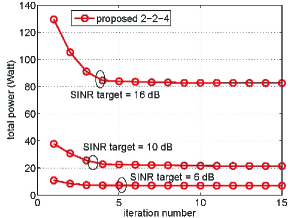
Figure 2: Convergence behavior of the decentralized algorithm for the QoS scheme.

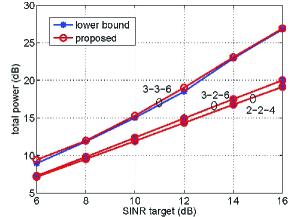
Figure 3: Comparison of the proposed algorithm with its lower bound for the QoS scheme.

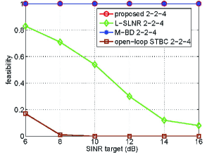
Figure 4: Comparison on feasibility of the different multicast beamforming algorithms for the QoS scheme.

In Fig. 3, we illustrate the efficiency of the SDR approach by comparing it with the lower bound, which is the solution of problem ${\bf P}_{1}(\gamma)$ in (13) where the rank-one constraint is relaxed. It can be seen that although we take the semidefinite relaxation, the proposed coordinated beamforming algorithm obtains the optimal performance in most cases.

We now compare the performance of the proposed SDR-based QoS beamforming in Algorithm 1 with two conventional multicell beamforming algorithms: multicell block diagonalization (M-BD) [19] and layered signal-to-leakage-plus-noise ratio (L-SLNR) [20]. Though these two algorithms were proposed for multicell networks with unicast traffic, they can be easily extended to multicasting. More specifically, for the M-BD algorithm, each base station chooses the beamforming vector which lies in the null space of the channels from the other $N-1$ base stations, i.e.,

$${\bf w}_{i}\in\mbox{Null}\left(\hat{{\bf H}}_{i}\right)$$ (44)

where $\hat{{\bf H}}_{i}=\left[{\bf h}_{1,i,1},...,{\bf h}_{1,i,K},...,{\bf h}_{i-1,i,1},...,{\bf h}_{i-1,i,K},\right.$ $\left.{\bf h}_{i+1,i,1},...,{\bf h}_{i+1,i,K},...,{\bf h}_{N,i,1},...,{\bf h}_{N,i,K}\right]^{H}$ and $\mbox{Null}(.)$ stands for the null space of a matrix. Then the QoS problem reduces to a power allocation problem and we can solve it to obtain the resulting power for each base station. For the L-SLNR algorithm, each base station chooses its beamforming vector as

$${\bf w}_{i}\propto\mbox{max.}\mbox{eigenvector}\left(\left[\sum\limits_{j\neq i}^{N}\sum\limits_{l=1}^{K}{\bf h}_{i,j,l}{\bf h}_{i,j,l}^{H}+\sigma^{2}{\bf I}\right]^{-1}\right.$$

$$\left.\cdot\left[\sum\limits_{l=1}^{K}{\bf h}_{i,i,l}{\bf h}_{i,i,l}^{H}\right]\right)~{}~{}~{}~{}~{}~{}~{}~{}~{}~{}~{}~{}~{}$$ (45)

which means that ${\bf w}_{i}$ should have the same direction as the eigenvector corresponding to the largest eigenvalue of the above matrix. We can similarly get the resulting beamforming vectors for the base stations by solving the reduced power allocation problem. As a performance benchmark, open-loop space time block coding (STBC) without requiring any CSI at each base station is also simulated. Fig. 4 shows the comparison on feasibility . Here, the feasibility percentage is obtained by counting the number of trials among the 200 channel realizations that each algorithm is able to find the solution to meet all the constraints. It can be seen that both the open-loop STBC and the L-SLNR beamformer almost do not work when SINR target $\gamma$ is large. This is expected as the open-loop STBC does not make any use of channel state information and serves purely as isotropic broadcasting. The L-SLNR beamformer, on the other hand, only tries to maximize the SLNR from the transmitter perspective and cannot guarantee the SINR maximization at the receiver end. From Fig. 4 it is also seen that the M-BD beamformer and the proposed coordinated beamformer are always feasible in the considered SINR target region. Here, the reason that the M-BD beamformer can work well is that the considered network is an interference-limited one and M-BD can null out all the interference for each user. The good performance of the proposed algorithm is expected as it can obtain the optimal solution in most cases under this particular setting (see Fig. 2). Therefore, in Fig. 5 we only compare the energy efficiency of the proposed algorithm with M-BD algorithm. We can see that the M-BD algorithm consumes much more power than the proposed algorithm. In particular, at target SINR of $10$dB, M-BD consumes $3$ dB more power in the $(2-2-4)$ system and $4$dB more power in the $(3-2-6)$ system. Notice that the M-BD algorithm requires that the number of transmitting antennas at each base station should be larger than the total number of receive antennas at all users. However, our proposed algorithm does not have this requirement.

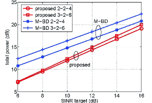
Figure 5: Comparison on energy efficiency of the different multicell multicast beamforming algorithms for the QoS scheme.

For the max-min SINR beamforming scheme, we assume the power constraint for each base station is the same. We first compare the the performance of the proposed Algorithm 2 with its upper bound in Fig. 6. Similar to the QoS scheme, we can see that the gap from the upper bound is very small and it achieves the optimal solution in most cases. Fig. 7 compares its performance with the existing algorithms. We can see that our proposed algorithm significantly outperforms the other ones over a large range of individual power constraint parameter. In particular, at the individual power constraint of $10$dB in the $(3-2-5)$ system, the worst-case SINR achieved by the proposed algorithm is $6$dB higher than L-SLNR, $8$dB higher than M-BD and $9$dB higher than open-loop STBC. From Fig. 7, it is also found that the M-BD algorithm performs the worst when the per base station power is small but is superior to the L-SLNR algorithm at large per base station power.

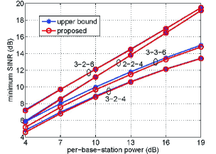
Figure 6: Comparison on the minimum SINR of the proposed algorithm with its upper bound for the MMS scheme.

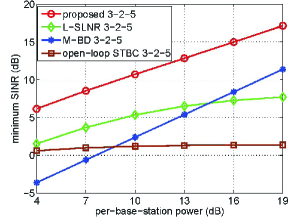
Figure 7: Comparison of the different multicell multicast beamforming algorithms for the MMS scheme.

V-B Effects of channel correlation

In practical scenarios, the channels among different users may be correlated with each other, especially for the users who are very near to each other in the geographical position. In order to model the correlated channels, we use the following Kronecker model [21] [22].

$${\bf H}_{kro}={\bf C}^{1/2}{\bf G},$$ (46)

where ${\bf H}_{kro}$ is a channel matrix whose rows are correlated with each other and ${\bf G}$ is a matrix with i.i.d. circularly symmetric Gaussian entries with zero mean and unit variance (This is for intracell channels by default. If it is intercell channel, the variance is $\varepsilon^{2}$). We model channel correlation matrix $\bf C$ as a Hermitian Toeplitz matrix with exponential entries $[{\bf C}]_{i,j}=r^{|i-j|}$ [23]. Here, $r$ can be seen as the correlation ratio and $0\leq r\leq 1$.

We first investigate the effects of intercell-user channel correlation on the feasibility of the QoS problem in Fig. 8. The correlation ratio $r$ is set to be $0.5$, $0.7$ and $0.9$, where $r=0$ stands for the independent channel. We can see that when the intercell-users’ channels are correlated, the feasibility decreases, which justifies our statement in Section III-A, i.e., the intercell-user channel correlation has a negative impact on the feasibility of the QoS problem.

Fig. 9 shows the effects of intracell-user channel correlation for the QoS beamforming scheme. The correlation ratio $r$ is also set to be 0.5, 0.7 and 0.9. From the results, we can see that when the intracell-user channels are correlated, it is helpful for the system. More specifically, the consumed power becomes less. We have observed the similar results on the usefulness of intracell-user channel correlation on the MMS scheme, which are ignored here due to page limit.

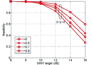
Figure 8: Feasibility of the proposed algorithm with correlated intercell-user channels for the QoS scheme.

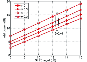
Figure 9: Total transmitted power with correlated intracell-user channels for the QoS scheme.

VI Conclusion

This paper considered two coordinated mulicast beamforming schemes for multicell networks. For the QoS scheme, we provided a necessary condition for the beamforming problem to be feasible when the network shares a common SINR target and proposed a decentralized algorithm to implement the coordinated beamforming. For the max-min SINR scheme, we considered individual base station power constraints and also proposed an efficient beamforming algorithm. Besides, we also investigated the impacts of intercell-user and intracell-user channel correlation on the multicast network.

There are several other issues to be further investigated for multicell multicast beamforming. First, finding the sufficient condition for the feasibility of the QoS problem remains open. Second, a decentralized algorithm to implement the beamforming design for the MMS scheme is to be designed. Last but not least, it is also interesting to consider robust beamforming when the channel state information at each base station is not perfect.

Appendix A Proof of Lemma 1

We first define the beamformer matrix ${\bf W}$ which is full-rank as below

$${\bf W}=\begin{bmatrix}{\bf w}_{1}&0&0&\cdots&0\\ 0&{\bf w}_{2}&0&\cdots&0\\ \vdots&\cdots&~{}&~{}\\ 0&0&0&\cdots&{\bf w}_{N}\end{bmatrix}~{}~{}~{}~{}~{}~{}~{}~{}~{}~{}~{}~{}~{}~{}~{}~{}~{}~{}~{}~{}~{}~{}~{}~{}~{}~{}~{}$$ (47)

Based on the fact that $\mbox{SINR}_{i,k}\leq\mbox{SIR}_{i,k}$, we have

$${\mbox{SINR}_{i,k}}=\frac{{|{\bf h}_{i,i,k}^{\emph{H}}{\bf w}_{i}|}^{2}}{\sum\limits^{N}_{j\neq i}{|{\bf h}_{j,i,k}^{\emph{H}}{\bf w}_{j}|}^{2}+\sigma^{2}_{i,k}}~{}~{}~{}~{}~{}~{}$$

$$\leq\frac{{|{\bf h}_{i,i,k}^{\emph{H}}{\bf w}_{i}|}^{2}}{\sum\limits^{N}_{j\neq i}{|{\bf h}_{j,i,k}^{\emph{H}}{\bf w}_{j}|}^{2}}=\frac{1}{\frac{1}{\eta_{i,k}}-1}$$ (48)

where we define the $\eta_{i,k}$ as below

$$\eta_{i,k}=\frac{|{\bf h}_{i,i,k}^{\emph{H}}{\bf w}_{i}|^{2}}{\sum\limits_{j=1}^{N}|{\bf h}_{j,i,k}^{\emph{H}}{\bf w}_{j}|^{2}}~{}~{}~{}~{}~{}~{}~{}~{}~{}~{}~{}~{}~{}~{}~{}~{}~{}~{}~{}~{}~{}~{}~{}~{}~{}~{}~{}~{}~{}$$

$$=\frac{|[{\bf H}_{k}{\bf W}]_{i,i}|^{2}}{\sum\limits_{j=1}^{N}|[{\bf H}_{k}{\bf W}]_{i,j}|^{2}}=\frac{|[{\bf H}_{k}{\bf W}]_{i,i}|^{2}}{|[{\bf H}_{k}{\bf W}{\bf W}^{\emph{H}}{\bf H}^{\emph{H}}_{k}]_{i,i}|}$$ (49)

the second equation in (49) is because (7) and (47). We also know the monotonicity of $f(x)=1/(1/x~{}-~{}1)$ when $x<1$. Comparing it with (48), we can bound the $\mbox{SINR}_{i,k}$ through bounding the associate $\eta_{i,k}$. Let the singular value decomposition(SVD) of ${\bf H}_{k}{\bf W}$ be denoted as ${\bf H}_{k}{\bf W}={\bf U}_{k}\bm{\Sigma}_{k}{\bf V}_{k}^{\emph{H}}$, where both ${\bf U}_{k}$ and ${\bf V}_{k}$ are $K\times r_{k}$ quasi-unitary matrix, i.e., their columns are orthogonal with each other. $\bm{\Sigma}_{k}$ is an $r_{k}\times r_{k}$ diagonal matrix whose elements are the singular values and $r_{k}=\mbox{rank}({\bf H}_{k}{\bf W})$. Then

$$\eta_{i,k}=\frac{|{\bf u}_{k,i}^{\emph{H}}\bm{\Sigma}_{k}{\bf v}_{k,i}|^{2}}{{\bf u}_{k,i}^{\emph{H}}\bm{\Sigma}_{k}^{2}{\bf u}_{k,i}},~{}i=1~{}2\cdots N,k=1~{}2\cdots K$$ (50)

where ${\bf u}_{k,i}$ and ${\bf v}_{k,i}$ are the ith columns of ${\bf U}_{k}$ and ${\bf V}_{k}$. According to Cauchy-Schwarz inequality, we have

$${|{\bf u}_{k,i}^{\emph{H}}\bm{\Sigma}_{k}{\bf v}_{k,i}|}^{2}\leq{\|{\bf u}_{k,i}^{\emph{H}}\bm{\Sigma}_{k}\|}^{2}\cdot{\|{\bf v}_{k,i}\|}^{2}~{}~{}~{}~{}~{}$$

$$=\left({\bf u}_{k,i}^{\emph{H}}\bm{\Sigma}_{k}^{2}{\bf u}_{k,i}\right)\left({\bf v}_{k,i}^{\emph{H}}{\bf v}_{k,i}\right)$$ (51)

Since ${\bf v}_{k,i}^{\emph{H}}{\bf v}_{k,i}=[({\bf H}_{k}{\bf W})^{\dagger}({\bf H}_{k}{\bf W})]_{i,i}$, we conclude that

$$\eta_{i,k}\leq[({\bf H}_{k}{\bf W})^{\dagger}({\bf H}_{k}{\bf W})]_{i,i}$$ (52)

Thus we have

$$\begin{split}\min_{i}\eta_{i,k}\leq{\frac{1}{N}}\sum_{i=1}^{N}\eta_{i,k}\leq{\frac{1}{N}}\sum_{i=1}^{N}[({\bf H}_{k}{\bf W})^{\dagger}({\bf H}_{k}{\bf W})]_{i,i}\\ ={\frac{1}{N}}\mbox{Tr}\{({\bf H}_{k}{\bf W})^{\dagger}{\bf H}_{k}{\bf W}\}=\frac{\mbox{rank}({\bf H}_{k}{\bf W})}{N}\leq\frac{\mbox{rank}({\bf H}_{k})}{N}\end{split}$$ (53)

Further we can get

$$\min_{i,k}\eta_{i,k}=\min_{k}\left\{\min_{i}\eta_{i,k}\right\}~{}~{}~{}~{}~{}~{}~{}~{}~{}~{}~{}~{}~{}~{}~{}~{}~{}~{}~{}~{}$$

$$\leq\min\{\frac{\mbox{rank}({\bf H}_{1})}{N},\frac{\mbox{rank}({\bf H}_{2})}{N},\cdots,\frac{\mbox{rank}({\bf H}_{K})}{N}\}$$ (54)

So if the problem (3) is feasible, then the minimum SINR should be larger than the threshold $\gamma$. Plugging (54) into (48), we can conclude that

$$\gamma\leq\min_{i,k}{\mbox{SINR}}_{i,k}\leq\left\{\frac{\mbox{rank}({\bf H}_{1})}{{\emph{N}}-\mbox{rank}({\bf H}_{1})},\cdots,\frac{\mbox{rank}({\bf H}_{K})}{{\emph{N}}-\mbox{rank}({\bf H}_{K})}\right\}$$ (55)

which completes the proof of Lemma 1.

Appendix B Proof of Theorem 1

We begin by computing the subgradient ${\bf g}_{i}$ from each subproblem. The Lagrangian of the $i$th subproblem is given by

$${\emph{L}}({\bf W}_{i},{\bf\Gamma},{\bm{\lambda}})={\mbox{Tr}}\{({\bf W}_{i})\}~{}~{}~{}~{}~{}~{}~{}~{}~{}~{}~{}~{}~{}~{}~{}~{}~{}~{}~{}~{}~{}~{}~{}~{}~{}~{}~{}~{}~{}~{}~{}~{}~{}~{}$$

$$-\sum_{k=1}^{K}\lambda_{i,i,k}\left[\frac{1}{\gamma_{i}}{\mbox{Tr}}\{{\bf H}_{i,i,k}{\bf W}_{i}\}-{\bf e}_{i,i,k}^{\emph{H}}{\bf\Gamma}-\sigma^{2}_{i,k}\right]~{}~{}$$

$$~{}+\sum_{j\neq i}^{N}\sum_{k=1}^{K}{\lambda_{i,j,k}}\bigg{[}{\mbox{Tr}}\{{\bf H}_{i,j,k}{\bf W}_{i}\}-{\bf e}_{i,j,k}^{\emph{H}}{\bf\Gamma}\bigg{]}~{}~{}~{}~{}~{}~{}~{}~{}~{}$$ (56)

Then the dual function $d_{i}({\bf\Gamma},{\bm{\lambda}})$ is

$$d_{i}({\bf\Gamma},{\bm{\lambda}})=\min\limits_{{\bf W}_{i}}{\emph{L}}({\bf W}_{i},{\bf\Gamma},{\bm{\lambda}})~{}~{}~{}~{}~{}~{}~{}~{}~{}~{}~{}~{}~{}~{}~{}~{}~{}~{}~{}~{}~{}~{}~{}~{}~{}~{}~{}~{}~{}~{}~{}~{}$$

$$=\left(\sum\limits_{k=1}^{K}\lambda_{i,i,k}{\bf e}_{i,i,k}^{T}-\sum\limits_{j\neq i}^{N}\sum\limits_{k=1}^{K}\lambda_{i,j,k}{\bf e}_{i,j,k}^{T}\right){\bf\Gamma}+f_{i}({\bm{\lambda}})$$ (57)

where

$$f_{i}({\bm{\lambda}})~{}~{}~{}~{}~{}~{}~{}~{}~{}~{}~{}~{}~{}~{}~{}~{}~{}~{}~{}~{}~{}~{}~{}~{}~{}~{}~{}~{}~{}~{}~{}~{}~{}~{}~{}~{}~{}~{}~{}~{}~{}~{}~{}~{}~{}~{}~{}~{}~{}~{}~{}~{}~{}~{}~{}~{}~{}~{}~{}~{}$$

$$=\min_{{\bf W}_{i}}\left({\mbox{Tr}}\{{\bf W}_{i}\}-\sum_{k=1}^{K}\lambda_{i,i,k}\left[\frac{1}{\gamma_{i}}{\mbox{Tr}}\{{\bf H}_{i,i,k}{\bf W}_{i}\}-\sigma^{2}_{i,k}\right]\right.$$

$$\left.+\sum_{j\neq i}^{N}\sum_{k=1}^{K}\lambda_{i,j,k}{\mbox{Tr}\{{\bf H}_{i,j,k}{\bf W}_{i}\}}\right)~{}~{}~{}~{}~{}~{}~{}~{}~{}~{}~{}~{}~{}~{}~{}~{}~{}~{}~{}~{}~{}~{}~{}~{}~{}$$ (58)

Since the problem ${\bf P}_{i}^{\mbox{sub}}(\gamma,{\bf\Gamma})$ is convex, then the strong duality holds which means that

$$P_{i}^{\star}({\bf\Gamma})=\max_{{\bm{\lambda}}\succeq\bf 0}d_{i}({\bf\Gamma},{\bm{\lambda}})$$ (59)

Denote ${\bm{\lambda}}^{\star}$ as the optimal Lagrange multiplier for the dual problem, then we have

$$P_{i}^{\star}({\bf\Gamma})=d_{i}({\bf\Gamma},{\bm{\lambda}}^{\star})~{}~{}~{}~{}~{}~{}~{}~{}~{}~{}~{}~{}~{}~{}~{}~{}~{}~{}~{}~{}~{}~{}~{}~{}~{}~{}~{}~{}~{}~{}~{}~{}~{}~{}~{}~{}~{}~{}~{}~{}~{}~{}~{}~{}$$

$$=\left(\sum_{k=1}^{K}\lambda_{i,i,k}^{\star}{\bf e}_{i,i,k}^{T}-\sum_{j\neq i}^{N}\sum_{k=1}^{K}\lambda_{i,j,k}^{\star}{\bf e}_{i,j,k}^{T}\right){\bf\Gamma}+f_{i}({\bm{\lambda}}^{\star})$$ (60)

Define ${\bf g}_{i}$ as

$${\bf g}_{i}\triangleq\sum\limits_{k=1}^{K}\lambda_{i,i,k}^{\star}{\bf e}_{i,i,k}-\sum\limits_{j\neq i}^{N}\sum\limits_{k=1}^{K}\lambda_{i,j,k}^{\star}{\bf e}_{i,j,k},$$ (61)

we have

$$P_{i}^{\star}({\bf\Gamma})={\bf g}_{i}^{H}{\bf\Gamma}+f_{i}({\bm{\lambda}}^{\star})~{}~{}~{}~{}~{}~{}~{}~{}~{}~{}~{}~{}~{}~{}~{}~{}~{}~{}~{}~{}~{}~{}~{}~{}~{}~{}~{}~{}~{}~{}~{}~{}~{}~{}~{}~{}~{}~{}$$

$$={\bf g}_{i}^{H}({\bf\Gamma}-\widetilde{{\bf\Gamma}})+{\bf g}_{i}^{H}\widetilde{{\bf\Gamma}}+f_{i}({\bm{\lambda}}^{\star})\leq{\bf g}_{i}^{H}({\bf\Gamma}-\widetilde{{\bf\Gamma}})+P_{i}^{\star}(\widetilde{{\bf\Gamma}})$$ (62)

which is equivalent to that

$$P_{i}^{\star}(\widetilde{{\bf\Gamma}})\geq P_{i}^{\star}({\bf\Gamma})+{\bf g}_{i}^{H}(\widetilde{{\bf\Gamma}}-{\bf\Gamma}).$$ (63)

It means that ${\bf g}_{i}$ is the subgradient of $P_{i}^{\star}({\bm{\Gamma}})$ and obtained for the $i$th subproblem.

In the same way, we can compute the global subgradient $\bf g$ of ${\bf P}^{\mbox{mas}}(\bm{\gamma},{\bf\Gamma})$ as below

$${\bf g} = \sum\limits_{i=1}^{N}\sum\limits_{k=1}^{K}\lambda_{i,i,k}^{\star}{\bf e}_{i,i,k}-\sum\limits_{i=1}^{N}\sum\limits_{j\neq i}^{N}\sum\limits_{k=1}^{K}\lambda_{i,j,k}^{\star}{\bf e}_{i,j,k}$$

$$= \sum\limits_{i=1}^{N}\left(\sum\limits_{k=1}^{K}\lambda_{i,i,k}^{\star}{\bf e}_{i,i,k}-\sum\limits_{j\neq i}^{N}\sum\limits_{k=1}^{K}\lambda_{i,j,k}^{\star}{\bf e}_{i,j,k}\right)$$

$$= \sum\limits_{i=1}^{N}{\bf g}_{i}$$ (64)

which completes the proof of Theorem 1.

References

- [1] N. D. Sidiropoulos, T. N. Davidson, and Z.-Q. Luo, “Transmit beamforming for physical-layer multicasting,” IEEE Transactions on Signal Processing, vol. 54, no. 6, Jun 2006.
- [2] E. Karipidis, N. D. Sidiropoulos, and Z.-Q. Luo, “Quality of service and max-min fair transmit beamforming to multiple cochannel multicast groups,” IEEE Transactions on Signal Processing, vol. 56, no. 3, Mar, 2008.
- [3] V. Ntranos, N. D. Sidiropoulos and L. Tassiulas, “On multicast beamforming for minimum outage,” IEEE Transactions on Wireless Communications, vol. 8, no. 6, Jun 2009.
- [4] S. Y. Park and D. J. Love, “Capacity limits of multiple antenna multicasting using antenna subset selection,” IEEE Transactions on Signal Processing, vol. 56, no. 6, Jun 2008.
- [5] Motorola Inc., “Long term evolution (LTE): A technical overview,” Technical White Paper,http://business.motorola.com /experienceltr/pdf/LTE%20Technical%20overview.pdf
- [6] A. Lozano, “Long-term transmit beamforming for wireless multicasting,” in Proc. ICASSP’ 07, April 2007, Honolulu, Hawaii.
- [7] S. Shamai(Shitz) and B. M. Zaidel, “Enhancing the cellular downlink capacity via co-processing at the transmitting end,” in Proc. IEEE Vehicle Technology Conference.(VTC), May 2001, vol. 3, pp. 1745-1749.
- [8] H. Zhang and H. Dai, “Cochannel interference mitigation and cooperative processing in downlink multicell multiuser MIMO networks,” EURASIP J. Wireless Commun. Netw., no. 2, 2004.
- [9] R. Mochaourab and E. Jorswieck, “Optimal beamforming in interference networks with perfect local channel information,” IEEE Transactions on Signal Processing, vol. 59, no. 3, March 2011.
- [10] D. P. Palomar, M. Chiang, “A tutorial on decomposition methods for network utility maximization,” IEEE Jouranl on Selected Areas in Communications, vol. 21, no. 8, Aug 2006.
- [11] M. Jordan, X. Gong, G. Ascheid, “Multicell Multicast Beamforming with Delayed SNR Feedback,” Proc. GLOBECOM 09, Nov, 2009.
- [12] G. Dartmann, X. Gong, G. Ascheid, “Low Complexity Cooperative Multicast Beamforming in Multiuser Multicell Downlink Networks”, Proc. CROWNCOM’ 2011, Jun, 2011.
- [13] G. Dartmann, X. Gong, G. Ascheid, “Cooperative Beamforming with Multiple Base Station Assignment Based on Correlation Knowledge”, Proc. VTC, 2010.
- [14] A. Wiesel, Y. C. Eldar, S. Shamai (Shitz), “Linear precoding via conic optimization for fixed MIMO receivers,” IEEE Transactions on Signal Processing, vol. 54, no. 1, Jan 2006.
- [15] M. Grant and S. Boyd. CVX: Matlab software for disciplined convex programming [online]. Available: http://stanford.edu.boyd/cvx.
- [16] S. Zhang, Y. Huang, “Complex quadratic optimization and semidefinite programming,” SIAM J. Optim., vol. 16, no. 3, Jan, 2006.
- [17] H. Dahrouj, W. Yu, “Coordinated beamforming for the multicell multi-antenna wireless system,” IEEE Transactions on Wireless Communications, vol. 9, no. 5, May 2010.
- [18] R. Zhang, S. Cui, “Cooperative interference management with MISO beamforming,” IEEE Transactions on Signal Processing, vol. 58, no. 10, Oct 2010.
- [19] R. Zhang, “Cooperative multi-cell block diagonalization with per-base-station power constraints,” IEEE Jouranl on Selected Areas in Communications, vol. 28, no. 9, Dec. 2010.
- [20] R. Zakhour and D. Gesbert “Distributed multicell-MISO precoding using the layered virtual SINR framework,” IEEE Transactions on Wireless Communications, vol. 9, no. 8, Aug. 2010.
- [21] X. Mestre and J. Fonollosa. “Capacity of MIMO channels: Asymptotic evaluation under correlated fading,” IEEE Jouranl on Selected Areas in Communications, vol. 21, no. 5, June 2003.
- [22] K. Werner, M. Janson and P. Stoica. “On estimation of covariance matrices with kronecher product structure,” IEEE Transactions on Signal Processing, vol. 56, no. 2, Feb 2008.
- [23] A. Paulraj, R. Nabar, and D. Gore, Introduction to Space-Time Wireless Communications. Cambridge, U.K.: Cambridge Univ. Press, 2003