Multi-Stage Multi-Task Feature Learning

Abstract

Multi-task sparse feature learning aims to improve the generalization performance by exploiting the shared features among tasks. It has been successfully applied to many applications including computer vision and biomedical informatics. Most of the existing multi-task sparse feature learning algorithms are formulated as a convex sparse regularization problem, which is usually suboptimal, due to its looseness for approximating an $\ell_{0}$-type regularizer. In this paper, we propose a non-convex formulation for multi-task sparse feature learning based on a novel non-convex regularizer. To solve the non-convex optimization problem, we propose a Multi-Stage Multi-Task Feature Learning (MSMTFL) algorithm; we also provide intuitive interpretations, detailed convergence and reproducibility analysis for the proposed algorithm. Moreover, we present a detailed theoretical analysis showing that MSMTFL achieves a better parameter estimation error bound than the convex formulation. Empirical studies on both synthetic and real-world data sets demonstrate the effectiveness of MSMTFL in comparison with the state of the art multi-task sparse feature learning algorithms.

Keywords: Multi-Task Learning, Multi-Stage, Non-convex, Sparse Learning

1 Introduction

Multi-task learning (MTL) (Caruana, 1997) exploits the relationships among multiple related tasks to improve the generalization performance. It has been successfully applied to many applications such as speech classification (Parameswaran and Weinberger, 2010), handwritten character recognition (Obozinski et al., 2006; Quadrianto et al., 2010) and medical diagnosis (Bi et al., 2008). One common assumption in multi-task learning is that all tasks should share some common structures including the prior or parameters of Bayesian models (Schwaighofer et al., 2005; Yu et al., 2005; Zhang et al., 2006), a similarity metric matrix (Parameswaran and Weinberger, 2010), a classification weight vector (Evgeniou and Pontil, 2004), a low rank subspace (Chen et al., 2010; Negahban and Wainwright, 2011) and a common set of shared features (Argyriou et al., 2008; Gong et al., 2012; Kim and Xing, 2009; Kolar et al., 2011; Lounici et al., 2009; Liu et al., 2009; Negahban and Wainwright, 2008; Obozinski et al., 2006; Yang et al., 2009; Zhang et al., 2010).

Multi-task feature learning, which aims to learn a common set of shared features, has received a lot of interests in machine learning recently, due to the popularity of various sparse learning formulations and their successful applications in many problems. In this paper, we focus on a specific multi-task feature learning setting, in which we learn the features specific to each task as well as the common features shared among tasks. Although many multi-task feature learning algorithms have been proposed in the past, many of them require the relevant features to be shared by all tasks. This is too restrictive in real-world applications (Jalali et al., 2010). To overcome this limitation, Jalali et al. (2010) proposed an $\ell_{1}+\ell_{1,\infty}$ regularized formulation, called dirty model, to leverage the common features shared among tasks. The dirty model allows a certain feature to be shared by some tasks but not all tasks. Jalali et al. (2010) also presented a theoretical analysis under the incoherence condition (Donoho et al., 2006; Obozinski et al., 2011) which is more restrictive than RIP (Candes and Tao, 2005; Zhang, 2012). The $\ell_{1}+\ell_{1,\infty}$ regularizer is a convex relaxation for the $\ell_{0}$-type one, in which a globally optimal solution can be obtained. However, a convex regularizer is known to too loose to approximate the $\ell_{0}$-type one and often achieves suboptimal performance (either require restrictive conditions or obtain a suboptimal error bound) (Zhang and Zhang, 2012; Zhang, 2010, 2012). To remedy the limitation, a non-convex regularizer can be used instead. However, the non-convex formulation is usually difficult to solve and a globally optimal solution can not be obtained in most practical problems. Moreover, the solution of the non-convex formulation heavily depends on the specific optimization algorithms employed. Even with the same optimization algorithm adopted, different initializations usually lead to different solutions. Thus, it is often challenging to analyze the theoretical behavior of a non-convex formulation.

Contributions: We propose a non-convex formulation, called capped-$\ell_{1}$,$\ell_{1}$ regularized model for multi-task feature learning. The proposed model aims to simultaneously learn the features specific to each task as well as the common features shared among tasks. We propose a Multi-Stage Multi-Task Feature Learning (MSMTFL) algorithm to solve the non-convex optimization problem. We also provide intuitive interpretations of the proposed algorithm from several aspects. In addition, we present a detailed convergence analysis for the proposed algorithm. To address the reproducibility issue of the non-convex formulation, we show that the solution generated by the MSMTFL algorithm is unique (i.e., the solution is reproducible) under a mild condition, which facilitates the theoretical analysis of the MSMTFL algorithm. Although the MSMTFL algorithm may not obtain a globally optimal solution, we show that this solution achieves good performance. Specifically, we present a detailed theoretical analysis on the parameter estimation error bound for the MSMTFL algorithm. Our analysis shows that, under the sparse eigenvalue condition which is weaker than the incoherence condition used in Jalali et al. (2010), MSMTFL improves the error bound during the multi-stage iteration, i.e., the error bound at the current iteration improves the one at the last iteration. Empirical studies on both synthetic and real-world data sets demonstrate the effectiveness of the MSMTFL algorithm in comparison with the state of the art algorithms.

Notations: Scalars and vectors are denoted by lower case letters and bold face lower case letters, respectively. Matrices and sets are denoted by capital letters and calligraphic capital letters, respectively. The $\ell_{1}$ norm, Euclidean norm, $\ell_{\infty}$ norm and Frobenius norm are denoted by $\|\cdot\|_{1},~{}\|\cdot\|$, $\|\cdot\|_{\infty}$ and $\|\cdot\|_{F}$, respectively. $|\cdot|$ denotes the absolute value of a scalar or the number of elements in a set, depending on the context. We define the $\ell_{p,q}$ norm of a matrix $X$ as $\|X\|_{p,q}=\left(\sum_{i}\left((\sum_{j}|x_{ij}|^{q})^{1/q}\right)^{p}\right)^{1/p}$. We define $\mathbb{N}_{n}$ as $\{1,\cdots,n\}$ and $N(\mu,\sigma^{2})$ as the normal distribution with mean $\mu$ and variance $\sigma^{2}$. For a $d\times m$ matrix $W$ and sets $\mathcal{I}_{i}\subseteq\mathbb{N}_{d}\times\{i\},\mathcal{I}\subseteq\mathbb{N}_{d}\times\mathbb{N}_{d}$, we let $\mathbf{w}_{\mathcal{I}_{i}}$ be the $d\times 1$ vector with the $j$-th entry being $w_{ji}$, if $(j,i)\in\mathcal{I}_{i}$, and $0$, otherwise. We also let $W_{\mathcal{I}}$ be a $d\times m$ matrix with the $(j,i)$-th entry being $w_{ji}$, if $(j,i)\in\mathcal{I}$, and $0$, otherwise.

Organization: In Section 2, we introduce a non-convex formulation and present the corresponding optimization algorithm. In Section 3, we discuss the convergence and reproducibility issues of the MSMTFL algorithm. In Section 4, we present a detailed theoretical analysis on the MSMTFL algorithm, in terms of the parameter estimation error bound. In Section 5, we provide a sketch of the proof of the presented theoretical results and the detailed proof is provided in the Appendix. In Section 6, we report the experimental results and we conclude the paper in Section 7.

2 The Proposed Formulation and the Optimization Algorithm

In this section, we first present a non-convex formulation for multi-task feature learning. Then, we show how to solve the corresponding optimization problem. Finally, we provide intuitive interpretations and discussions for the proposed algorithm.

2.1 A Non-convex Formulation

Assume we are given $m$ learning tasks associated with training data $\left\{(X_{1},\mathbf{y}_{1}),\cdots,(X_{m},\mathbf{y}_{m})\right\}$, where $X_{i}\in\mathbb{R}^{n_{i}\times d}$ is the data matrix of the $i$-th task with each row as a sample; $\mathbf{y}_{i}\in\mathbb{R}^{n_{i}}$ is the response of the $i$-th task; $d$ is the data dimensionality; $n_{i}$ is the number of samples for the $i$-th task. We consider learning a weight matrix $W=[\mathbf{w}_{1},\cdots,\mathbf{w}_{m}]\in\mathbb{R}^{d\times m}$ consisting of the weight vectors for $m$ linear predictive models: $\mathbf{y}_{i}\approx\mathbf{f}_{i}(X_{i})=X_{i}\mathbf{w}_{i},~{}i\in\mathbb{N}_{m}$. In this paper, we propose a non-convex multi-task feature learning formulation to learn these $m$ models simultaneously, based on the capped-$\ell_{1}$,$\ell_{1}$ regularization. Specifically, we first impose the $\ell_{1}$ penalty on each row of $W$, obtaining a column vector. Then, we impose the capped-$\ell_{1}$ penalty (Zhang, 2010, 2012) on that vector. Formally, we formulate our proposed model as follows:

$$\min_{W\in\mathbb{R}^{d\times m}}\left\{l(W)+\lambda\sum_{j=1}^{d}\min\left(\|\mathbf{w}^{j}\|_{1},\theta\right)\right\},$$ (1)

where $l(W)$ is an empirical loss function of $W$; $\lambda~{}(>0)$ is a parameter balancing the empirical loss and the regularization; $\theta~{}(>0)$ is a thresholding parameter; $\mathbf{w}^{j}$ is the $j$-th row of the matrix $W$. In this paper, we focus on the following quadratic loss function:

$$l(W)=\sum_{i=1}^{m}\frac{1}{mn_{i}}\left\|X_{i}\mathbf{w}_{i}-\mathbf{y}_{i}\right\|^{2}.$$ (2)

Intuitively, due to the capped-$\ell_{1},\ell_{1}$ penalty, the optimal solution of Eq. (1) denoted as $W^{\star}$ has many zero rows. For a nonzero row $(\mathbf{w}^{\star})^{k}$, some entries may be zero, due to the $\ell_{1}$-norm imposed on each row of $W$. Thus, under the formulation in Eq. (1), some features can be shared by some tasks but not all the tasks. Therefore, the proposed formulation can leverage the common features shared among tasks.

2.2 Optimization Algorithm

The formulation in Eq. (1) is non-convex and is difficult to solve. In this paper, we propose an algorithm called Multi-Stage Multi-Task Feature Learning (MSMTFL) to solve the optimization problem (see details in Algorithm 1). In this algorithm, a key step is how to efficiently solve Eq. (3). Observing that the objective function in Eq. (3) can be decomposed into the sum of a differential loss function and a non-differential regularization term, we employ FISTA (Beck and Teboulle, 2009) to solve the sub-problem. In the following, we present some intuitive interpretations of the proposed algorithm from several aspects.

1 Initialize $\lambda_{j}^{(0)}=\lambda$;

2 for $\ell=1,2,\cdots$ do

3       Let $\hat{W}^{(\ell)}$ be a solution of the following problem:

$$\min_{W\in\mathbb{R}^{d\times m}}\left\{l(W)+\sum_{j=1}^{d}\lambda_{j}^{(\ell-1)}\|\mathbf{w}^{j}\|_{1}\right\}.$$ (3)

4      Let $\lambda_{j}^{(\ell)}=\lambda I(\|(\hat{\mathbf{w}}^{(\ell)})^{j}\|_{1}<\theta)~{}(j=1,\cdots,d)$, where $(\hat{\mathbf{w}}^{(\ell)})^{j}$ is the $j$-th row of $\hat{W}^{(\ell)}$ and $I(\cdot)$ denotes the $\{0,1\}$-valued indicator function.

5 end for

Algorithm 1 MSMTFL: Multi-Stage Multi-Task Feature Learning

2.2.1 Locally Linear Approximation

First, we define two auxiliary functions:

$$\mathbf{h}:\mathbb{R}^{d\times m}\mapsto\mathbb{R}^{d}_{+},~{}\mathbf{h}(W)=\left[\|\mathbf{w}^{1}\|_{1},\cdots,\|\mathbf{w}^{d}\|_{1}\right]^{T},$$

$$g:\mathbb{R}^{d}_{+}\mapsto\mathbb{R}_{+},~{}g(\mathbf{u})=\sum_{j=1}^{d}\min(u_{j},\theta).$$

We note that $g(\cdot)$ is a concave function and we say that a vector $\mathbf{s}\in\mathbb{R}^{d}$ is a sub-gradient of $g$ at $\mathbf{v}\in\mathbb{R}^{d}_{+}$, if for all vector $\mathbf{u}\in\mathbb{R}^{d}_{+}$, the following inequality holds:

$$g(\mathbf{u})\leq g(\mathbf{v})+\langle\mathbf{s},\mathbf{u}-\mathbf{v}\rangle,$$

where $\langle\cdot\rangle$ denotes the inner product. Using the functions defined above, Eq. (1) can be equivalently rewritten as follows:

$$\min_{W\in\mathbb{R}^{d\times m}}\left\{l(W)+\lambda g(\mathbf{h}(W))\right\}.$$ (4)

Based on the definition of the sub-gradient for a concave function given above, we can obtain an upper bound of $g(\mathbf{h}(W))$ using a locally linear approximation at $\mathbf{h}(\hat{W}^{(\ell)})$:

$$g(\mathbf{h}(W))\leq g(\mathbf{h}(\hat{W}^{(\ell)}))+\left\langle\mathbf{s}^{(\ell)},\mathbf{h}(W)-\mathbf{h}(\hat{W}^{(\ell)})\right\rangle,$$

where $\mathbf{s}^{(\ell)}$ is a sub-gradient of $g(\mathbf{u})$ at $\mathbf{u}=\mathbf{h}(\hat{W}^{(\ell)})$. Furthermore, we can obtain an upper bound of the objective function in Eq. (4), if the solution $\hat{W}^{(\ell)}$ at the $\ell$-th iteration is available:

$$\forall W\in\mathbb{R}^{d\times m}:l(W)+\lambda g(\mathbf{h}(W))\leq l(W)+\lambda g(\mathbf{h}(\hat{W}^{(\ell)}))+\lambda\left\langle\mathbf{s}^{(\ell)},\mathbf{h}(W)-\mathbf{h}(\hat{W}^{(\ell)})\right\rangle.$$ (5)

It can be shown that a sub-gradient of $g(\mathbf{u})$ at $\mathbf{u}=\mathbf{h}(\hat{W}^{(\ell)})$ is

$$\mathbf{s}^{(\ell)}=\left[I(\|(\hat{\mathbf{w}}^{(\ell)})^{1}\|_{1}<\theta),\cdots,I(\|(\hat{\mathbf{w}}^{(\ell)})^{d}\|_{1}<\theta)\right]^{T},$$ (6)

which is used in Step 4 of Algorithm 1. Since both $\lambda$ and $\mathbf{h}(\hat{W}^{(\ell)})$ are constant with respect to $W$, we have

$$\hat{W}^{(\ell+1)} =\mathop{\arg\min}_{W}\left\{l(W)+\lambda g(\mathbf{h}(\hat{W}^{(\ell)}))+\lambda\left\langle\mathbf{s}^{(\ell)},\mathbf{h}(W)-\mathbf{h}(\hat{W}^{(\ell)})\right\rangle\right\}$$

$$=\mathop{\arg\min}_{W}\left\{l(W)+\lambda(\mathbf{s}^{(\ell)})^{T}\mathbf{h}(W)\right\},$$

which, as shown in Step 3 of Algorithm 1, obtains the next iterative solution by minimizing the upper bound of the objective function in Eq. (4). Thus, in the viewpoint of the locally linear approximation, we can understand Algorithm 1 as follows: The original formulation in Eq. (4) is non-convex and is difficult to solve; the proposed algorithm minimizes an upper bound in each step, which is convex and can be solved efficiently. It is closely related to the Concave Convex Procedure (CCCP) (Yuille and Rangarajan, 2003). In addition, we can easily verify that the objective function value decreases monotonically as follows:

$$l(\hat{W}^{(\ell+1)})+\lambda g(\mathbf{h}(\hat{W}^{(\ell+1)})) \leq l(\hat{W}^{(\ell+1)})+\lambda g(\mathbf{h}(\hat{W}^{(\ell)}))+\lambda\left\langle\mathbf{s}^{(\ell)},\mathbf{h}(\hat{W}^{(\ell+1)})-\mathbf{h}(\hat{W}^{(\ell)})\right\rangle$$

$$\leq l(\hat{W}^{(\ell)})+\lambda g(\mathbf{h}(\hat{W}^{(\ell)}))+\lambda\left\langle\mathbf{s}^{(\ell)},\mathbf{h}(\hat{W}^{(\ell)})-\mathbf{h}(\hat{W}^{(\ell)})\right\rangle$$

$$=l(\hat{W}^{(\ell)})+\lambda g(\mathbf{h}(\hat{W}^{(\ell)})),$$

where the first inequality is due to Eq. (5) and the second inequality follows from the fact that $\hat{W}^{(\ell+1)}$ is a minimizer of the right hand side of Eq. (5).

An important issue we should mention is that a monotonic decrease of the objective function value does not guarantee the convergence of the algorithm, even if the objective function is strictly convex and continuously differentiable (see an example in the book (Bertsekas, 1999, Fig 1.2.6)). In Section 3.1, we will formally discuss the convergence issue.

2.2.2 Block Coordinate Descent

Recall that $g(\mathbf{u})$ is a concave function. We can define its conjugate function as (Rockafellar, 1970):

$$g^{\star}(\mathbf{v})=\inf_{\mathbf{u}}\{\mathbf{v}^{T}\mathbf{u}-g(\mathbf{u})\}.$$

Since $g(\mathbf{u})$ is also a closed function (i.e., the epigraph of $g(\mathbf{u})$ is convex), the conjugate function of $g^{\star}(\mathbf{v})$ is the original function $g(\mathbf{u})$ (Bertsekas, 1999, Chap. 5.4), that is:

$$g(\mathbf{u})=\inf_{\mathbf{v}}\{\mathbf{u}^{T}\mathbf{v}-g^{\star}(\mathbf{v})\}.$$ (7)

Substituting Eq. (7) with $\mathbf{u}=\mathbf{h}(W)$ into Eq. (4), we can reformulate Eq. (4) as:

$$\min_{W,\mathbf{v}}\left\{f(W,\mathbf{v})=l(W)+\lambda\mathbf{v}^{T}\mathbf{h}(W)-\lambda g^{\star}(\mathbf{v})\right\}$$ (8)

A straightforward algorithm for optimizing Eq. (8) is the block coordinate descent (Grippo and Sciandrone, 2000; Tseng, 2001) summarized below:

• Fix $W=\hat{W}^{(\ell)}$:

  $$\hat{\mathbf{v}}^{(\ell)} =\mathop{\arg\min}_{\mathbf{v}}\left\{l(\hat{W}^{(\ell)})+\lambda\mathbf{v}^{T}\mathbf{h}(\hat{W}^{(\ell)})-\lambda g^{\star}(\mathbf{v})\right\}$$

  $$=\mathop{\arg\min}_{\mathbf{v}}\left\{\mathbf{v}^{T}\mathbf{h}(\hat{W}^{(\ell)})-g^{\star}(\mathbf{v})\right\}.$$ (9)

  Based on Eq. (7) and the Danskin’s Theorem (Bertsekas, 1999, Proposition B.25), one solution of Eq. (9) is given by a sub-gradient of $g(\mathbf{u})$ at $\mathbf{u}=\mathbf{h}(\hat{W}^{(\ell)})$. That is, we can choose $\hat{\mathbf{v}}^{(\ell)}=\mathbf{s}^{(\ell)}$ given in Eq. (6). Apparently, Eq. (9) is equivalent to Step 4 in Algorithm 1.

• Fix $\mathbf{v}=\hat{\mathbf{v}}^{(\ell)}=\left[I(\|(\hat{\mathbf{w}}^{(\ell)})^{1}\|_{1}<\theta),\cdots,I(\|(\hat{\mathbf{w}}^{(\ell)})^{d}\|_{1}<\theta)\right]^{T}$:

  $$\hat{W}^{(\ell+1)} =\mathop{\arg\min}_{W}\left\{l(W)+\lambda(\hat{\mathbf{v}}^{(\ell)})^{T}\mathbf{h}(W)-\lambda g^{\star}(\hat{\mathbf{v}}^{(\ell)})\right\}$$

  $$=\mathop{\arg\min}_{W}\left\{l(W)+\lambda(\hat{\mathbf{v}}^{(\ell)})^{T}\mathbf{h}(W)\right\},$$ (10)

  which corresponds to Step 3 of Algorithm 1.

The block coordinate descent procedure is intuitive, however, it is non-trivial to analyze its convergence behavior. We will present the convergence analysis in Section 3.1.

2.2.3 Discussions

If we terminate the algorithm with $\ell=1$, the MSMTFL algorithm is equivalent to the $\ell_{1}$ regularized multi-task feature learning algorithm (Lasso). Thus, the solution obtained by MSMTFL can be considered as a multi-stage refinement of that of Lasso. Basically, the MSMTFL algorithm solves a sequence of weighted Lasso problems, where the weights $\lambda_{j}$’s are set as the product of the parameter $\lambda$ in Eq. (1) and a $\{0,1\}$-valued indicator function. Specifically, a penalty is imposed in the current stage if the $\ell_{1}$-norm of some row of $W$ in the last stage is smaller than the threshold $\theta$; otherwise, no penalty is imposed. In other words, MSMTFL in the current stage tends to shrink the small rows of $W$ and keep the large rows of $W$ in the last stage. However, Lasso (corresponds to $\ell=1$) penalizes all rows of $W$ in the same way. It may incorrectly keep the irrelevant rows (which should have been zero rows) or shrink the relevant rows (which should have been large rows) to be zero vectors. MSMTFL overcomes this limitation by adaptively penalizing the rows of $W$ according to the solution generated in the last stage. One important question is whether the MSMTFL algorithm can improve the performance during the multi-stage iteration. In Section 4, we will theoretically show that the MSMTFL algorithm indeed achieves the stagewise improvement in terms of the parameter estimation error bound. That is, the error bound in the current stage improves the one in the last stage. Empirical studies in Section 6 also validate the presented theoretical analysis.

3 Convergence and Reproducibility Analysis

In this section, we first present the convergence analysis. Then, we discuss the reproducibility issue for the MSMTFL algorithm.

3.1 Convergence Analysis

The main convergence result is summarized in the following theorem, which is based on the block coordinate descent interpretation.

Theorem 1

Let $(W^{\star},\mathbf{v}^{\star})$ be a limit point of the sequence $\{\hat{W}^{(\ell)},\hat{\mathbf{v}}^{(\ell)}\}$ generated by the block coordinate descent algorithm. Then $W^{\star}$ is a critical point of Eq. (1).

Proof  Based on Eq. (9) and Eq. (10), we have

$$f(\hat{W}^{(\ell)},\hat{\mathbf{v}}^{(\ell)}) \leq f(\hat{W}^{(\ell)},\mathbf{v}),~{}\forall\mathbf{v}\in\mathbb{R}^{d},$$

$$f(\hat{W}^{(\ell+1)},\hat{\mathbf{v}}^{(\ell)}) \leq f(W,\hat{\mathbf{v}}^{(\ell)}),~{}\forall W\in\mathbb{R}^{d\times m}.$$ (11)

It follows that

$$f(\hat{W}^{(\ell+1)},\hat{\mathbf{v}}^{(\ell+1)})\leq f(\hat{W}^{(\ell+1)},\hat{\mathbf{v}}^{(\ell)})\leq f(\hat{W}^{(\ell)},\hat{\mathbf{v}}^{(\ell)}),$$

which indicates that the sequence $\{f(\hat{W}^{(\ell)},\hat{\mathbf{v}}^{(\ell)})\}$ is monotonically decreasing. Since $(W^{\star},\mathbf{v}^{\star})$ is a limit point of $\{\hat{W}^{(\ell)},\hat{\mathbf{v}}^{(\ell)}\}$, there exists a subsequence $\mathcal{K}$ such that

$$\lim_{\ell\in\mathcal{K}\rightarrow\infty}(\hat{W}^{(\ell)},\hat{\mathbf{v}}^{(\ell)})=(W^{\star},\mathbf{v}^{\star}).$$

We observe that

$$f(W,\mathbf{v}) =l(W)+\lambda\mathbf{v}^{T}\mathbf{h}(W)-\lambda g^{\star}(\mathbf{v})$$

$$\geq l(W)+\lambda g(\mathbf{h}(W))\geq 0,$$

where the first inequality above is due to Eq. (7). Thus, $\{f(\hat{W}^{(\ell)},\hat{\mathbf{v}}^{(\ell)})\}_{\ell\in\mathcal{K}}$ is bounded below. Together with the fact that $\{f(\hat{W}^{(\ell)},\hat{\mathbf{v}}^{(\ell)})\}$ is decreasing, $\lim_{\ell\rightarrow\infty}f(\hat{W}^{(\ell)},\hat{\mathbf{v}}^{(\ell)})>-\infty$ exists. Since $f(W,\mathbf{v})$ is continuous, we have

$$\lim_{\ell\rightarrow\infty}f(\hat{W}^{(\ell)},\hat{\mathbf{v}}^{(\ell)})=\lim_{\ell\in\mathcal{K}\rightarrow\infty}f(\hat{W}^{(\ell)},\hat{\mathbf{v}}^{(\ell)})=f(W^{\star},\mathbf{v}^{\star}).$$

Taking limits on both sides of Eq. (11) with $\ell\in\mathcal{K}\rightarrow\infty$, we have

$$f(W^{\star},\mathbf{v}^{\star})\leq f(W,\mathbf{v}^{\star}),~{}\forall W\in\mathbb{R}^{d\times m},$$

which implies

$$W^{\star} \in\mathop{\arg\min}_{W}f(W,\mathbf{v}^{\star})$$

$$=\mathop{\arg\min}_{W}\left\{l(W)+\lambda(\mathbf{v}^{\star})^{T}\mathbf{h}(W)-\lambda g^{\star}(\mathbf{v}^{\star})\right\}$$

$$=\mathop{\arg\min}_{W}\left\{l(W)+\lambda(\mathbf{v}^{\star})^{T}\mathbf{h}(W)\right\}.$$ (12)

Therefore, the zero matrix $O$ must be a sub-gradient of the objective function in Eq. (12) at $W=W^{\star}$ :

$$O\in\partial l(W^{\star})+\lambda\partial\left((\mathbf{v}^{\star})^{T}\mathbf{h}(W^{\star})\right)=\partial l(W^{\star})+\lambda\sum_{j=1}^{d}v^{\star}_{j}\partial\left(\|(\mathbf{w}^{\star})^{j}\|_{1}\right),$$ (13)

where $\partial l(W^{\star})$ denotes the sub-differential (which is a set composed of all sub-gradients) of $l(W)$ at $W=W^{\star}$. We observe that

$$\hat{\mathbf{v}}^{(\ell)}\in\partial g(\mathbf{u})|_{\mathbf{u}=\mathbf{h}(\hat{W}^{(\ell)})},$$

which implies that $\forall\mathbf{x}\in\mathbb{R}^{d}_{+}$:

$$g(\mathbf{x})\leq g(\mathbf{h}(\hat{W}^{(\ell)}))+\left\langle\hat{\mathbf{v}}^{(\ell)},\mathbf{x}-\mathbf{h}(\hat{W}^{(\ell)})\right\rangle.$$

Taking limits on both sides of the above inequality with $\ell\in\mathcal{K}\rightarrow\infty$, we have:

$$g(\mathbf{x})\leq g(\mathbf{h}(W^{\star}))+\left\langle\mathbf{v}^{\star},\mathbf{x}-\mathbf{h}(W^{\star})\right\rangle,$$

which implies that $\mathbf{v}^{\star}$ is a sub-gradient of $g(\mathbf{u})$ at $\mathbf{u}=\mathbf{h}(W^{\star})$, that is:

$$\mathbf{v}^{\star}\in\partial g(\mathbf{u})|_{\mathbf{u}=\mathbf{h}(W^{\star})}.$$ (14)

Substituting Eq. (14) into Eq. (13), we obtain:

$$O\in\partial l(W^{\star})+\lambda\sum_{j=1}^{d}\partial\min(\|(\mathbf{w}^{\star})^{j}\|_{1},\theta).$$

Therefore, $W^{\star}$ is a critical point of Eq. (1). This completes the proof of Theorem 1.  

Remark 2

Note that the above theorem holds by assuming that there exists a limit point. Next, we need to prove that the sequence $\{\hat{W}^{(\ell)},\hat{\mathbf{v}}^{(\ell)}\}$ has a limit point. For any bounded initial point $\{\hat{W}^{(0)},\hat{\mathbf{v}}^{(0)}\}$, based on Eq. (7), Eq. (8) and the monotonicity of $f(\hat{W}^{(\ell)},\hat{\mathbf{v}}^{(\ell)})$, we have:

$$l(\hat{W}^{(\ell)})+\lambda g(\mathbf{h}(\hat{W}^{(\ell)}))\leq f(\hat{W}^{(\ell)},\hat{\mathbf{v}}^{(\ell)})\leq f(\hat{W}^{(0)},\hat{\mathbf{v}}^{(0)})<+\infty,\forall\ell\geq 1.$$ (15)

Assume that the sequence $\{\hat{W}^{(\ell)},\hat{\mathbf{v}}^{(\ell)}\}$ is unbounded, that is, there exist some $i,j$ such that $|\hat{W}_{ij}^{(\ell)}|\rightarrow+\infty$. It implies that $l(\hat{W}^{(\ell)})+\lambda g(\mathbf{h}(\hat{W}^{(\ell)}))\rightarrow+\infty$ (We exclude the case that some columns of $X_{i}$ are zero vectors. Otherwise, we can simply remove the corresponding zero columns.) and hence $f(\hat{W}^{(\ell)},\hat{\mathbf{v}}^{(\ell)})\rightarrow+\infty$. This leads to a contradiction with Eq. (15). Thus, the sequence $\{\hat{W}^{(\ell)},\hat{\mathbf{v}}^{(\ell)}\}$ is bounded and there exists at least one limit point $(W^{\star},\mathbf{v}^{\star})$, since any bounded sequence has limit points.

Due to the equivalence between Algorithm 1 and the block coordinate descent algorithm above, Theorem 1 and its remark indicate that the sequence $\{\hat{W}^{(\ell)}\}$ generated by Algorithm 1 has at least one limit point that is also a critical point of Eq. (1). The remaining issue is to analyze the performance of the critical point. In the sequel, we will conduct analysis in two aspects: reproducibility and the parameter estimation performance.

3.2 Reproducibility of The Algorithm

In general, it is difficult to analyze the performance of a non-convex formulation, as different solutions can be obtained due to different initializations. One natural question is whether the solution generated by Algorithm 1 (based on the initialization of $\lambda_{j}^{(0)}=\lambda$ in Step 1) is reproducible. In other words, is the solution of Algorithm 1 unique? If we can guarantee that, for any $\ell\geq 1$, the solution $\hat{W}^{(\ell)}$ of Eq. (3) is unique, then the solution generated by Algorithm 1 is unique. That is, the solution is reproducible. The main result is summarized in the following theorem:

Theorem 3

If $X_{i}\in\mathbb{R}^{n_{i}\times d}~{}(i\in\mathbb{N}_{m})$ has entries drawn from a continuous probability distribution on $R^{n_{i}d}$, then, for any $\ell\geq 1$, the optimization problem in Eq. (3) has a unique solution with probability one.

Proof  Eq. (3) can be decomposed into $m$ independent smaller minimization problems:

$$\hat{\mathbf{w}}^{(\ell)}_{i}=\mathop{\arg\min}_{\mathbf{w}_{i}\in\mathbb{R}^{d}}\frac{1}{mn_{i}}\|X_{i}\mathbf{w}_{i}-\mathbf{y}_{i}\|^{2}+\sum_{j=1}^{d}\lambda^{(\ell-1)}_{j}|w_{ji}|.$$

Next, we only need to prove the solution of the above optimization problem is unique. To simplify the notations, we unclutter the above equation (by ignoring some superscripts and subscripts) as follows:

$$\hat{\mathbf{w}}=\mathop{\arg\min}_{\mathbf{w}\in\mathbb{R}^{d}}\frac{1}{mn}\|X\mathbf{w}-\mathbf{y}\|^{2}+\sum_{j=1}^{d}\lambda_{j}|w_{j}|,$$ (16)

The first order optimal condition is $\forall j\in\mathbb{N}_{d}$:

$$\frac{2}{mn}\mathbf{x}_{j}^{T}(\mathbf{y}-X\hat{\mathbf{w}})=\lambda_{j}\mathrm{sign}(\hat{w}_{j}),$$ (17)

where $\mathrm{sign}(\hat{w}_{j})=1$, if $\hat{w}_{j}>0$; $\mathrm{sign}(\hat{w}_{j})=-1$, if $\hat{w}_{j}<0$; and $\mathrm{sign}(\hat{w}_{j})\in[-1,1]$, otherwise. We define

$$\mathcal{E} =\left\{j\in\mathbb{N}_{d}:\frac{2}{mn}|\mathbf{x}_{j}^{T}(\mathbf{y}-X\hat{\mathbf{w}})|=\lambda_{j}\right\},$$

$$\mathbf{s}=\mathrm{sign}\left(\frac{2}{mn}X_{\mathcal{E}}^{T}(\mathbf{y}-X\hat{\mathbf{w}})\right),$$

where $X_{\mathcal{E}}$ denotes the matrix composed of the columns of $X$ indexed by $\mathcal{E}$. Then, the optimal solution $\hat{\mathbf{w}}$ of Eq. (16) satisfies

$$\hat{\mathbf{w}}_{\mathbb{N}_{d}\setminus\mathcal{E}}=\mathbf{0},$$

$$\hat{\mathbf{w}}_{\mathcal{E}}=\mathop{\arg\min}_{\mathbf{w}_{\mathcal{E}}\in\mathbb{R}^{|\mathcal{E}|}}\frac{1}{mn}\|X_{\mathcal{E}}\mathbf{w}_{\mathcal{E}}-\mathbf{y}\|^{2}+\sum_{j\in\mathcal{E}}\lambda_{j}|w_{j}|,~{}s.t.~{}s_{j}w_{j}\geq 0,j\in\mathcal{E},$$ (18)

where $\mathbf{w}_{\mathcal{E}}$ denotes the vector composed of entries of $\mathbf{w}$ indexed by $\mathcal{E}$. Since $X\in\mathbb{R}^{n_{i}\times d}$ is drawn from the continuous probability distribution, $X$ has columns in general positions with probability one and hence $\mathrm{rank}(X_{\mathcal{E}})=|\mathcal{E}|$ (or equivalently $\mathrm{Null}(X_{\mathcal{E}})=\{\mathbf{0}\}$), due to Lemma 3, Lemma 4 and their discussions in Tibshirani (2012). Therefore, the objective function in Eq. (18) is strictly convex, which implies that $\hat{\mathbf{w}}_{\mathcal{E}}$ is unique. Thus, the optimal solution $\hat{\mathbf{w}}$ of Eq. (16) is also unique and so is the optimization problem in Eq. (3) for any $\ell\geq 1$. This completes the proof of Theorem 3.  
Theorem 3 is important in the sense that it makes the theoretical analysis for the parameter estimation performance of Algorithm 1 possible. Although the solution may not be globally optimal, we show in the next section that the solution has good performance in terms of the parameter estimation error bound.

4 Parameter Estimation Error Bound

In this section, we theoretically analyze the parameter estimation performance of the solution obtained by the MSMTFL algorithm. To simplify the notations in the theoretical analysis, we assume that the number of samples for all the tasks are the same. However, our theoretical analysis can be easily extended to the case where the tasks have different sample sizes.

We first present a sub-Gaussian noise assumption which is very common in the analysis of sparse learning literature (Zhang and Zhang, 2012; Zhang, 2008, 2009, 2010, 2012).

Assumption 1

Let $\bar{W}=[\bar{\mathbf{w}}_{1},\cdots,\bar{\mathbf{w}}_{m}]\in\mathbb{R}^{d\times m}$ be the underlying sparse weight matrix and $\mathbf{y}_{i}=X_{i}\bar{\mathbf{w}}_{i}+\bm{\delta}_{i},~{}\mathbb{E}\mathbf{y}_{i}=X_{i}\bar{\mathbf{w}}_{i}$, where $\bm{\delta}_{i}\in\mathbb{R}^{n}$ is a random vector with all entries $\delta_{ji}~{}(j\in\mathbb{N}_{n},i\in\mathbb{N}_{m})$ being independent sub-Gaussians: there exists $\sigma>0$ such that $\forall j\in\mathbb{N}_{n},i\in\mathbb{N}_{m},t\in\mathbb{R}$:

$$\mathbb{E}_{\delta_{ji}}\exp(t\delta_{ji})\leq\exp\left(\frac{\sigma^{2}t^{2}}{2}\right).$$

Remark 4

We call the random variable satisfying the condition in Assumption 1 sub-Gaussian, since its moment generating function is bounded by that of a zero mean Gaussian random variable. That is, if a normal random variable $x\sim N(0,\sigma^{2})$, then we have:

$$\mathbb{E}\exp(tx) =\int_{-\infty}^{\infty}\exp(tx)\frac{1}{\sqrt{2\pi}\sigma}\exp\left(-\frac{x^{2}}{2\sigma^{2}}\right)dx$$

$$=\exp(\sigma^{2}t^{2}/2)\int_{-\infty}^{\infty}\frac{1}{\sqrt{2\pi}\sigma}\exp\left(-\frac{(x-\sigma^{2}t)^{2}}{2\sigma^{2}}\right)dx$$

$$=\exp(\sigma^{2}t^{2}/2).$$

Remark 5

Based on the Hoeffding’s Lemma, for any random variable $x\in[a,b]$ and $\mathbb{E}x=0$, we have $\mathbb{E}(\exp(tx))\leq\exp\left(\frac{t^{2}(b-a)^{2}}{8}\right)$. Therefore, both zero mean Gaussian and zero mean bounded random variables are sub-Gaussians. Thus, the sub-Gaussian noise assumption is more general than the Gaussian noise assumption which is commonly used in the multi-task learning literature (Jalali et al., 2010; Lounici et al., 2009).

We next introduce the following sparse eigenvalue concept which is also common in the analysis of sparse learning literature (Zhang and Huang, 2008; Zhang and Zhang, 2012; Zhang, 2009, 2010, 2012).

Definition 6

Given $1\leq k\leq d$, we define

$$\rho^{+}_{i}(k)=\sup_{\mathbf{w}}\left\{\frac{\|X_{i}\mathbf{w}\|^{2}}{n\|\mathbf{w}\|^{2}}:\|\mathbf{w}\|_{0}\leq k\right\},~{}\rho^{+}_{max}(k)=\max_{i\in\mathbb{N}_{m}}\rho^{+}_{i}(k),$$

$$\rho^{-}_{i}(k)=\inf_{\mathbf{w}}\left\{\frac{\|X_{i}\mathbf{w}\|^{2}}{n\|\mathbf{w}\|^{2}}:\|\mathbf{w}\|_{0}\leq k\right\},~{}\rho^{-}_{min}(k)=\min_{i\in\mathbb{N}_{m}}\rho^{-}_{i}(k).$$

Remark 7

$\rho^{+}_{i}(k)~{}(\rho^{-}_{i}(k))$ is in fact the maximum (minimum) eigenvalue of $(X_{i})_{\mathcal{S}}^{T}(X_{i})_{\mathcal{S}}/n$, where $\mathcal{S}$ is a set satisfying $|\mathcal{S}|\leq k$ and $(X_{i})_{\mathcal{S}}$ is a submatrix composed of the columns of $X_{i}$ indexed by $\mathcal{S}$. In the MTL setting, we need to exploit the relations of $\rho^{+}_{i}(k)~{}(\rho^{-}_{i}(k))$ among multiple tasks.

We present our parameter estimation error bound on MSMTFL in the following theorem:

Theorem 8

Let Assumption 1 hold. Define $\bar{\mathcal{F}}_{i}=\{(j,i):\bar{w}_{ji}\neq 0\}$ and $\bar{\mathcal{F}}=\cup_{i\in\mathbb{N}_{m}}\bar{\mathcal{F}}_{i}$. Denote $\bar{r}$ as the number of nonzero rows of $\bar{W}$. We assume that

$$\forall(j,i)\in\bar{\mathcal{F}},\|\bar{\mathbf{w}}^{j}\|_{1}\geq 2\theta$$ (19)

$$\mathrm{and}~{} \frac{\rho^{+}_{i}(s)}{\rho^{-}_{i}(2\bar{r}+2s)}\leq 1+\frac{s}{2\bar{r}},$$ (20)

where $s$ is some integer satisfying $s\geq\bar{r}$. If we choose $\lambda$ and $\theta$ such that for some $s\geq\bar{r}$:

$$\lambda \geq 12\sigma\sqrt{\frac{2\rho^{+}_{max}(1)\ln(2dm/\eta)}{n}},$$ (21)

$$\theta \geq\frac{11m\lambda}{\rho^{-}_{min}(2\bar{r}+s)},$$ (22)

then the following parameter estimation error bound holds with probability larger than $1-\eta$:

$$\|\hat{W}^{(\ell)}-\bar{W}\|_{2,1}\leq 0.8^{\ell/2}\frac{9.1m\lambda\sqrt{\bar{r}}}{\rho^{-}_{min}(2\bar{r}+s)}+\frac{39.5m\sigma\sqrt{\rho^{+}_{max}(\bar{r})(7.4\bar{r}+2.7\ln(2/\eta))/n}}{\rho^{-}_{min}(2\bar{r}+s)},$$ (23)

where $\hat{W}^{(\ell)}$ is a solution of Eq. (3).

Remark 9

Eq. (19) assumes that the $\ell_{1}$-norm of each nonzero row of $\bar{W}$ is away from zero. This requires the true nonzero coefficients should be large enough, in order to distinguish them from the noise. Eq. (20) is called the sparse eigenvalue condition (Zhang, 2012), which requires the eigenvalue ratio $\rho^{+}_{i}(s)/\rho^{-}_{i}(s)$ to grow sub-linearly with respect to $s$. Such a condition is very common in the analysis of sparse regularization (Zhang and Huang, 2008; Zhang, 2009) and it is slightly weaker than the RIP condition (Candes and Tao, 2005; Huang and Zhang, 2010; Zhang, 2012).

Remark 10

When $\ell=1$ (corresponds to Lasso), the first term of the right-hand side of Eq. (23) dominates the error bound in the order of

$$\|\hat{W}^{Lasso}-\bar{W}\|_{2,1}=O\left(m\sqrt{\bar{r}\ln(dm/\eta)/n}\right),$$ (24)

since $\lambda$ satisfies the condition in Eq. (21). Note that the first term of the right-hand side of Eq. (23) shrinks exponentially as $\ell$ increases. When $\ell$ is sufficiently large in the order of $O(\ln(m\sqrt{\bar{r}/n})+\ln\ln(dm))$, this term tends to zero and we obtain the following parameter estimation error bound:

$$\|\hat{W}^{(\ell)}-\bar{W}\|_{2,1}=O\left(m\sqrt{\bar{r}/n+\ln(1/\eta)/n}\right).$$ (25)

Jalali et al. (2010) gave an $\ell_{\infty,\infty}$-norm error bound $\|\hat{W}^{Dirty}-\bar{W}\|_{\infty,\infty}=O\left(\sqrt{\ln(dm/\eta)/n}\right)$ as well as a sign consistency result between $\hat{W}$ and $\bar{W}$. A direct comparison between these two bounds is difficult due to the use of different norms. On the other hand, the worst-case estimate of the $\ell_{2,1}$-norm error bound of the algorithm in Jalali et al. (2010) is in the same order with Eq. (24), that is: $\|\hat{W}^{Dirty}-\bar{W}\|_{2,1}=O\left(m\sqrt{\bar{r}\ln(dm/\eta)/n}\right)$. When $dm$ is large and the ground truth has a large number of sparse rows (i.e., $\bar{r}$ is a small constant), the bound in Eq. (25) is significantly better than the ones for the Lasso and Dirty model.

Remark 11

Jalali et al. (2010) presented an $\ell_{\infty,\infty}$-norm parameter estimation error bound and hence a sign consistency result can be obtained. The results are derived under the incoherence condition which is more restrictive than the RIP condition and hence more restrictive than the sparse eigenvalue condition in Eq. (20). From the viewpoint of the parameter estimation error, our proposed algorithm can achieve a better bound under weaker conditions. Please refer to (Van De Geer and Bühlmann, 2009; Zhang, 2009, 2012) for more details about the incoherence condition, the RIP condition, the sparse eigenvalue condition and their relationships.

Remark 12

The capped-$\ell_{1}$ regularized formulation in Zhang (2010) is a special case of our formulation when $m=1$. However, extending the analysis from the single task to the multi-task setting is nontrivial. Different from previous work on multi-stage sparse learning which focuses on a single task (Zhang, 2010, 2012), we study a more general multi-stage framework in the multi-task setting. We need to exploit the relationship among tasks, by using the relations of sparse eigenvalues $\rho^{+}_{i}(k)~{}(\rho^{-}_{i}(k))$ and treating the $\ell_{1}$-norm on each row of the weight matrix as a whole for consideration. Moreover, we simultaneously exploit the relations of each column and each row of the matrix.

5 Proof Sketch of Theorem 8

In this section, we present a proof sketch of Theorem 8. We first provide several important lemmas (detailed proofs are available in the Appendix) and then complete the proof of Theorem 8 based on these lemmas.

Lemma 13

Let $\bar{\Upsilon}=[\bar{\bm{\epsilon}}_{1},\cdots,\bar{\bm{\epsilon}}_{m}]$ with $\bar{\bm{\epsilon}}_{i}=[\bar{\epsilon}_{1i},\cdots,\bar{\epsilon}_{di}]^{T}=\frac{1}{n}X_{i}^{T}(X_{i}\bar{\mathbf{w}}_{i}-\mathbf{y}_{i})~{}(i\in\mathbb{N}_{m})$. Define $\bar{\mathcal{H}}\supseteq\bar{\mathcal{F}}$ such that $(j,i)\in\bar{\mathcal{H}}~{}(\forall i\in\mathbb{N}_{m})$, provided there exists $(j,g)\in\bar{\mathcal{F}}$ ($\bar{\mathcal{H}}$ is a set consisting of the indices of all entries in the nonzero rows of $\bar{W}$). Under the conditions of Assumption 1 and the notations of Theorem 8, the followings hold with probability larger than $1-\eta$:

$$\|\bar{\Upsilon}\|_{\infty,\infty}\leq\sigma\sqrt{\frac{2\rho^{+}_{max}(1)\ln(2dm/\eta)}{n}},$$ (26)

$$\|\bar{\Upsilon}_{\bar{\mathcal{H}}}\|^{2}_{F}\leq m\sigma^{2}\rho^{+}_{max}(\bar{r})(7.4\bar{r}+2.7\ln(2/\eta))/n.$$ (27)

Lemma 13 gives bounds on the residual correlation ($\bar{\Upsilon}$) with respect to $\bar{W}$. We note that Eq. (26) and Eq. (27) are closely related to the assumption on $\lambda$ in Eq. (21) and the second term of the right-hand side of Eq. (23) (error bound), respectively. This lemma provides a fundamental basis for the proof of Theorem 8.

Lemma 14

Use the notations of Lemma 13 and consider $\mathcal{G}_{i}\subseteq\mathbb{N}_{d}\times\{i\}$ such that $\bar{\mathcal{F}}_{i}\cap\mathcal{G}_{i}=\emptyset~{}(i\in\mathbb{N}_{m})$. Let $\hat{W}=\hat{W}^{(\ell)}$ be a solution of Eq. (3) and $\Delta\hat{W}=\hat{W}-\bar{W}$. Denote $\hat{\bm{\lambda}}_{i}=\hat{\bm{\lambda}}_{i}^{(\ell-1)}=[\lambda^{(\ell-1)}_{1},\cdots,\lambda^{(\ell-1)}_{d}]^{T}$. Let $\hat{\lambda}_{\mathcal{G}_{i}}=\min_{(j,i)\in\mathcal{G}_{i}}\hat{\lambda}_{ji},~{}\hat{\lambda}_{\mathcal{G}}=\min_{i\in\mathcal{G}_{i}}\hat{\lambda}_{\mathcal{G}_{i}}$ and $\hat{\lambda}_{0i}=\max_{j}\hat{\lambda}_{ji},~{}\hat{\lambda}_{0}=\max_{i}\hat{\lambda}_{0i}$. If $2\|\bar{\bm{\epsilon}}_{i}\|_{\infty}<\hat{\lambda}_{\mathcal{G}_{i}}$, then the following inequality holds at any stage $\ell\geq 1$:

$$\sum_{i=1}^{m}\sum_{(j,i)\in\mathcal{G}_{i}}|\hat{w}_{ji}^{(\ell)}|\leq\frac{2\|\bar{\Upsilon}\|_{\infty,\infty}+\hat{\lambda}_{0}}{\hat{\lambda}_{\mathcal{G}}-2\|\bar{\Upsilon}\|_{\infty,\infty}}\sum_{i=1}^{m}\sum_{(j,i)\in\mathcal{G}_{i}^{c}}|\Delta\hat{w}_{ji}^{(\ell)}|.$$

Denote $\mathcal{G}=\cup_{i\in\mathbb{N}_{m}}\mathcal{G}_{i},~{}\bar{\mathcal{F}}=\cup_{i\in\mathbb{N}_{m}}{\bar{\mathcal{F}}_{i}}$ and notice that $\bar{\mathcal{F}}\cap\mathcal{G}=\emptyset\Rightarrow\Delta\hat{W}^{(\ell)}=\hat{W}^{(\ell)}$. Lemma 14 says that $\|\Delta\hat{W}_{\mathcal{G}}^{(\ell)}\|_{1,1}=\|\hat{W}_{\mathcal{G}}^{(\ell)}\|_{1,1}$ is upper bounded in terms of $\|\Delta\hat{W}_{\mathcal{G}^{c}}^{(\ell)}\|_{1,1}$, which indicates that the error of the estimated coefficients locating outside of $\bar{\mathcal{F}}$ should be small enough. This provides an intuitive explanation why the parameter estimation error of our algorithm can be small.

Lemma 15

Using the notations of Lemma 14, we denote $\mathcal{G}=\mathcal{G}_{(\ell)}=\bar{\mathcal{H}}^{c}\cap\{(j,i):\hat{\lambda}_{ji}^{(\ell-1)}=\lambda\}=\cup_{i\in\mathbb{N}_{m}}\mathcal{G}_{i}$ with $\bar{\mathcal{H}}$ being defined as in Lemma 13 and $\mathcal{G}_{i}\subseteq\mathbb{N}_{d}\times\{i\}$. Let $\mathcal{J}_{i}$ be the indices of the largest $s$ coefficients (in absolute value) of $\hat{\mathbf{w}}_{\mathcal{G}_{i}}$, $\mathcal{I}_{i}=\mathcal{G}_{i}^{c}\cup\mathcal{J}_{i}$, $\mathcal{I}=\cup_{i\in\mathbb{N}_{m}}{\mathcal{I}_{i}}$ and $\bar{\mathcal{F}}=\cup_{i\in\mathbb{N}_{m}}{\bar{\mathcal{F}}_{i}}$. Then, the following inequalities hold at any stage $\ell\geq 1$:

$$\|\Delta\hat{W}^{(\ell)}\|_{2,1}\leq\frac{\left(1+1.5\sqrt{\frac{2\bar{r}}{s}}\right)\sqrt{8m\left(4\|\bar{\Upsilon}_{\mathcal{G}_{(\ell)}^{c}}\|_{F}^{2}+\sum_{(j,i)\in\bar{\mathcal{F}}}(\hat{\lambda}_{ji}^{(\ell-1)})^{2}\right)}}{\rho^{-}_{min}(2\bar{r}+s)},$$ (28)

$$\|\Delta\hat{W}^{(\ell)}\|_{2,1}\leq\frac{9.1m\lambda\sqrt{\bar{r}}}{\rho^{-}_{min}(2\bar{r}+s)}.$$ (29)

Lemma 15 is established based on Lemma 14, by considering the relationship between Eq. (21) and Eq. (26), and the specific definition of $\mathcal{G}=\mathcal{G}_{(\ell)}$. Eq. (28) provides a parameter estimation error bound in terms of $\ell_{2,1}$-norm by $\|\bar{\Upsilon}_{\mathcal{G}_{(\ell)}^{c}}\|_{F}^{2}$ and the regularization parameters $\hat{\lambda}_{ji}^{(\ell-1)}$ (see the definition of $\hat{\lambda}_{ji}~{}(\hat{\lambda}_{ji}^{(\ell-1)})$ in Lemma 14). This is the result directly used in the proof of Theorem 8. Eq. (29) states that the error bound is upper bounded in terms of $\lambda$, the right-hand side of which constitutes the shrinkage part of the error bound in Eq. (23).

Lemma 16

Let $\hat{\lambda}_{ji}=\lambda I\left(\|\hat{\mathbf{w}}^{j}\|_{1}<\theta,j\in\mathbb{N}_{d}\right),\forall i\in\mathbb{N}_{m}$ with some $\hat{W}\in\mathbb{R}^{d\times m}$. $\bar{\mathcal{H}}\supseteq\bar{\mathcal{F}}$ is defined in Lemma 13. Then under the condition of Eq. (19), we have:

$$\sum_{(j,i)\in\bar{\mathcal{F}}}\hat{\lambda}_{ji}^{2}\leq\sum_{(j,i)\in\bar{\mathcal{H}}}\hat{\lambda}_{ji}^{2}\leq m\lambda^{2}\|\bar{W}_{\bar{\mathcal{H}}}-\hat{W}_{\bar{\mathcal{H}}}\|_{2,1}^{2}/\theta^{2}.$$

Lemma 16 establishes an upper bound of $\sum_{(j,i)\in\bar{\mathcal{F}}}\hat{\lambda}_{ji}^{2}$ by $\|\bar{W}_{\bar{\mathcal{H}}}-\hat{W}_{\bar{\mathcal{H}}}\|_{2,1}^{2}$, which is critical for building the recursive relationship between $\|\hat{W}^{(\ell)}-\bar{W}\|_{2,1}$ and $\|\hat{W}^{(\ell-1)}-\bar{W}\|_{2,1}$ in the proof of Theorem 8. This recursive relation is crucial for the shrinkage part of the error bound in Eq. (23).

5.1 Proof of Theorem 8

Proof  For notational simplicity, we denote the right-hand side of Eq. (27) as:

$$u=m\sigma^{2}\rho^{+}_{max}(\bar{r})(7.4\bar{r}+2.7\ln(2/\eta))/n.$$ (30)

Based on $\bar{\mathcal{H}}\subseteq\mathcal{G}_{(\ell)}^{c}$, Lemma 13 and Eq. (21), the followings hold with probability larger than $1-\eta$:

$$\|\bar{\Upsilon}_{\mathcal{G}_{(\ell)}^{c}}\|_{F}^{2} =\|\bar{\Upsilon}_{\bar{\mathcal{H}}}\|_{F}^{2}+\|\bar{\Upsilon}_{\mathcal{G}_{(\ell)}^{c}\setminus\bar{\mathcal{H}}}\|_{F}^{2}$$

$$\leq u+|\mathcal{G}_{(\ell)}^{c}\setminus\bar{\mathcal{H}}|\|\bar{\Upsilon}\|_{\infty,\infty}^{2}$$

$$\leq u+\lambda^{2}|\mathcal{G}_{(\ell)}^{c}\setminus\bar{\mathcal{H}}|/144$$

$$\leq u+(1/144)m\lambda^{2}\theta^{-2}\|\hat{W}^{(\ell-1)}_{\mathcal{G}_{(\ell)}^{c}\setminus\bar{\mathcal{H}}}-\bar{W}_{\mathcal{G}_{(\ell)}^{c}\setminus\bar{\mathcal{H}}}\|_{2,1}^{2},$$ (31)

where the last inequality follows from

$$\forall (j,i)\in\mathcal{G}_{(\ell)}^{c}\setminus\bar{\mathcal{H}},\|(\hat{\mathbf{w}}^{(\ell-1)})^{j}\|_{1}^{2}/\theta^{2}=\|(\hat{\mathbf{w}}^{(\ell-1)})^{j}-\bar{\mathbf{w}}^{j}\|_{1}^{2}/\theta^{2}\geq 1$$

$$\Rightarrow| \mathcal{G}_{(\ell)}^{c}\setminus\bar{\mathcal{H}}|\leq m\theta^{-2}\|\hat{W}^{(\ell-1)}_{\mathcal{G}_{(\ell)}^{c}\setminus\bar{\mathcal{H}}}-\bar{W}_{\mathcal{G}_{(\ell)}^{c}\setminus\bar{\mathcal{H}}}\|_{2,1}^{2}.$$

According to Eq. (28), we have:

$$\|\hat{W}^{(\ell)}-\bar{W}\|_{2,1}^{2}=\|\Delta\hat{W}^{(\ell)}\|_{2,1}^{2}$$

$$\leq\frac{8m\left(1+1.5\sqrt{\frac{2\bar{r}}{s}}\right)^{2}\left(4\|\bar{\Upsilon}_{\mathcal{G}_{(\ell)}^{c}}\|_{F}^{2}+\sum_{(j,i)\in\bar{\mathcal{F}}}(\hat{\lambda}_{ji}^{(\ell-1)})^{2}\right)}{(\rho^{-}_{min}(2\bar{r}+s))^{2}}$$

$$\leq\frac{78m\left(4u+(37/36)m\lambda^{2}\theta^{-2}\left\|\hat{W}^{(\ell-1)}-\bar{W}\right\|_{2,1}^{2}\right)}{(\rho^{-}_{min}(2\bar{r}+s))^{2}}$$

$$\leq\frac{312mu}{(\rho^{-}_{min}(2\bar{r}+s))^{2}}+0.8\left\|\hat{W}^{(\ell-1)}-\bar{W}\right\|_{2,1}^{2}$$

$$\leq\cdots\leq 0.8^{\ell}\left\|\hat{W}^{(0)}-\bar{W}\right\|_{2,1}^{2}+\frac{312mu}{(\rho^{-}_{min}(2\bar{r}+s))^{2}}\frac{1-0.8^{\ell}}{1-0.8}$$

$$\leq 0.8^{\ell}\frac{9.1^{2}m^{2}\lambda^{2}\bar{r}}{(\rho^{-}_{min}(2\bar{r}+s))^{2}}+\frac{1560mu}{(\rho^{-}_{min}(2\bar{r}+s))^{2}}.$$

In the above derivation, the first inequality is due to Eq. (28); the second inequality is due to the assumption $s\geq\bar{r}$ in Theorem 8, Eq. (31) and Lemma 16; the third inequality is due to Eq. (22); the last inequality follows from Eq. (29) and $1-0.8^{\ell}\leq 1~{}(\ell\geq 1)$. Thus, following the inequality $\sqrt{a+b}\leq\sqrt{a}+\sqrt{b}~{}(\forall a,b\geq 0)$, we obtain:

$$\|\hat{W}^{(\ell)}-\bar{W}\|_{2,1}\leq 0.8^{\ell/2}\frac{9.1m\lambda\sqrt{\bar{r}}}{\rho^{-}_{min}(2\bar{r}+s)}+\frac{39.5\sqrt{mu}}{\rho^{-}_{min}(2\bar{r}+s)}.$$

Substituting Eq. (30) into the above inequality, we verify Theorem 8.  

Remark 17

The assumption $s\geq\bar{r}$ used in the above proof indicates that at each stage, the zero entries of $\hat{W}^{(\ell)}$ should be greater than $m\bar{r}$ (see definition of $s$ in Lemma 15). This requires the solution obtained by Algorithm 1 at each stage is sparse, which is consistent with the sparsity of $\bar{W}$ in Assumption 1.

6 Experiments

In this section, we present empirical studies on both synthetic and real-world data sets. In the synthetic data experiments, we present the performance of the MSMTFL algorithm in terms of the parameter estimation error. In the real-world data experiments, we show the performance of the MSMTFL algorithm in terms of the prediction error.

6.1 Competing Algorithms

We present the empirical studies by comparing our proposed MSMTFL algorithm with three competing multi-task feature learning algorithms: $\ell_{1}$-norm multi-task feature learning algorithm (Lasso), $\ell_{1,2}$-norm multi-task feature learning algorithm (L1,2) (Obozinski et al., 2006) and dirty model multi-task feature learning algorithm (DirtyMTL) (Jalali et al., 2010). In our experiments, we employ the quadratic loss function in Eq. (2) for all the compared algorithms.

6.2 Synthetic Data Experiments

We generate synthetic data by setting the number of tasks as $m$ and each task has $n$ samples which are of dimensionality $d$; each element of the data matrix $X_{i}\in\mathbb{R}^{n\times d}~{}(i\in\mathbb{N}_{m})$ for the $i$-th task is sampled i.i.d. from the Gaussian distribution $N(0,1)$ and we then normalize all columns to length $1$; each entry of the underlying true weight $\bar{W}\in\mathbb{R}^{d\times m}$ is sampled i.i.d. from the uniform distribution in the interval $[-10,10]$; we randomly set $90\%$ rows of $\bar{W}$ as zero vectors and $80\%$ elements of the remaining nonzero entries as zeros; each entry of the noise $\bm{\delta}_{i}\in\mathbb{R}^{n}$ is sampled i.i.d. from the Gaussian distribution $N(0,\sigma^{2})$; the responses are computed as $\mathbf{y}_{i}=X_{i}\bar{\mathbf{w}}_{i}+\bm{\delta}_{i}~{}(i\in\mathbb{N}_{m})$.

We first report the averaged parameter estimation error $\|\hat{W}-\bar{W}\|_{2,1}$ vs. Stage ($\ell$) plots for MSMTFL (Figure 1). We observe that the error decreases as $\ell$ increases, which shows the advantage of our proposed algorithm over Lasso. This is consistent with the theoretical result in Theorem 8. Moreover, the parameter estimation error decreases quickly and converges in a few stages.

We then report the averaged parameter estimation error $\|\hat{W}-\bar{W}\|_{2,1}$ in comparison with four algorithms in different parameter settings (Figure 2). For a fair comparison, we compare the smallest estimation errors of the four algorithms in all the parameter settings (Zhang, 2009, 2010). As expected, the parameter estimation error of the MSMTFL algorithm is the smallest among the four algorithms. This empirical result demonstrates the effectiveness of the MSMTFL algorithm. We also have the following observations: (a) When $\lambda$ is large enough, all four algorithms tend to have the same parameter estimation error. This is reasonable, because the solutions $\hat{W}$’s obtained by the four algorithms are all zero matrices, when $\lambda$ is very large. (b) The performance of the MSMTFL algorithm is similar for different $\theta$’s, when $\lambda$ exceeds a certain value.

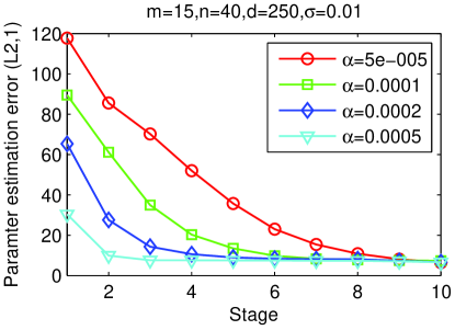
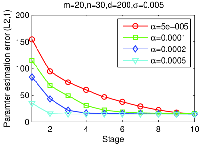
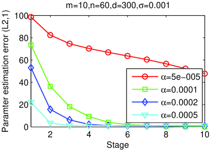
Figure 1: Averaged parameter estimation error $\|\hat{W}-\bar{W}\|_{2,1}$ vs. Stage ($\ell$) plots for MSMTFL on the synthetic data set (averaged over 10 runs). Here we set $\lambda=\alpha\sqrt{\ln(dm)/n},~{}\theta=50m\lambda$. Note that $\ell=1$ corresponds to Lasso; the results show the stage-wise improvement over Lasso.

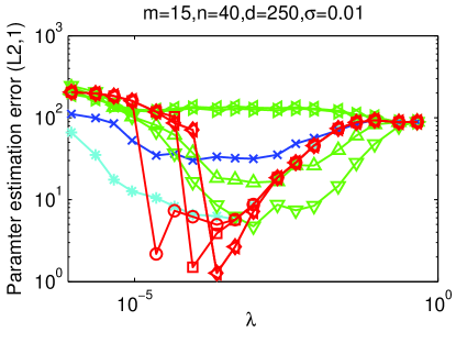
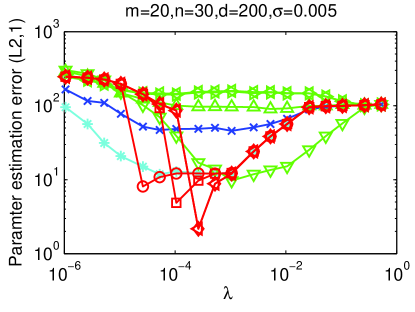
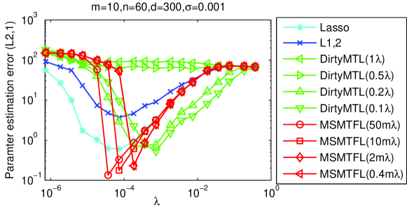
Figure 2: Averaged parameter estimation error $\|\hat{W}-\bar{W}\|_{2,1}$ vs. $\lambda$ plots on the synthetic data set (averaged over 10 runs). MSMTFL has the smallest parameter estimation error among the four algorithms. Both DirtyMTL and MSMTFL have two parameters; we set $\lambda_{s}/\lambda_{b}=1,0.5,0.2,0.1$ for DirtyMTL ($1/m\leq\lambda_{s}/\lambda_{b}\leq 1$ was adopted in Jalali et al. (2010)) and $\theta/\lambda=50m,10m,2m,0.4m$ for MSMTFL.

6.3 Real-World Data Experiments

We conduct experiments on two real-world data sets: MRI and Isolet data sets.

The MRI data set is collected from the ANDI database, which contains 675 patients’ MRI data preprocessed using FreeSurfer. The MRI data include 306 features and the response (target) is the Mini Mental State Examination (MMSE) score coming from 6 different time points: M06, M12, M18, M24, M36, and M48. We remove the samples which fail the MRI quality controls and have missing entries. Thus, we have 6 tasks with each task corresponding to a time point and the sample sizes corresponding to 6 tasks are 648, 642, 293, 569, 389 and 87, respectively.

The Isolet data set is collected from 150 speakers who speak the name of each English letter of the alphabet twice. Thus, there are 52 samples from each speaker. The speakers are grouped into 5 subsets which respectively include 30 similar speakers, and the subsets are named Isolet1, Isolet2, Isolet3, Isolet4, and Isolet5. Thus, we naturally have 5 tasks with each task corresponding to a subset. The 5 tasks respectively have 1560, 1560, 1560, 1558, and 1559 samples, where each sample includes 617 features and the response is the English letter label (1-26).

Table 1: Comparison of four multi-task feature learning algorithms on the MRI data set in terms of averaged nMSE and aMSE (standard deviation), which are averaged over 10 random splittings.

measure	traning ratio	Lasso	L1,2	DirtyMTL	MSMTFL
nMSE	$0.15$	0.6651(0.0280)	0.6633(0.0470)	0.6224(0.0265)	0.5539(0.0154)
	$0.20$	0.6254(0.0212)	0.6489(0.0275)	0.6140(0.0185)	0.5542(0.0139)
	$0.25$	0.6105(0.0186)	0.6577(0.0194)	0.6136(0.0180)	0.5507(0.0142)
aMSE	$0.15$	0.0189(0.0008)	0.0187(0.0010)	0.0172(0.0006)	0.0159(0.0004)
	$0.20$	0.0179(0.0006)	0.0184(0.0005)	0.0171(0.0005)	0.0161(0.0004)
	$0.25$	0.0172(0.0009)	0.0183(0.0006)	0.0167(0.0008)	0.0157(0.0006)

In the experiments, we treat the MMSE and letter labels as the regression values for the MRI data set and the Isolet data set, respectively. For both data sets, we randomly extract the training samples from each task with different training ratios ($15\%,20\%$ and $25\%$) and use the rest of samples to form the test set. We evaluate the four multi-task feature learning algorithms in terms of normalized mean squared error (nMSE) and averaged means squared error (aMSE), which are commonly used in multi-task learning problems (Zhang and Yeung, 2010; Zhou et al., 2011; Gong et al., 2012). For each training ratio, both nMSE and aMSE are averaged over 10 random splittings of training and test sets and the standard deviation is also shown. All parameters of the four algorithms are tuned via 3-fold cross validation.

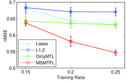
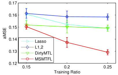
Figure 3: Averaged test error (nMSE and aMSE) vs. training ratio plots on the Isolet data set. The results are averaged over 10 random splittings.

Table 1 and Figure 3 show the experimental results in terms of averaged nMSE (aMSE) and the standard deviation. From these results, we observe that: (a) Our proposed MSMTFL algorithm outperforms all the competing feature learning algorithms on both data sets, with the smallest regression errors (nMSE and aMSE) as well as the smallest standard deviations. (b) On the MRI data set, the MSMTFL algorithm performs well even in the case of a small training ratio. The performance for the $15\%$ training ratio is comparable to that for the $25\%$ training ratio. (c) On the Isolet data set, when the training ratio increases from $15\%$ to $25\%$, the performance of the MSMTFL algorithm increases and the superiority of the MSMTFL algorithm over the other three algorithms is more significant. Our results demonstrate the effectiveness of the proposed algorithm.

7 Conclusions

In this paper, we propose a non-convex formulation for multi-task feature learning, which learns the specific features of each task as well as the common features shared among tasks. The non-convex formulation adopts the capped-$\ell_{1}$,$\ell_{1}$ regularizer to better approximate the $\ell_{0}$-type one than the commonly used convex regularizer. To solve the non-convex optimization problem, we propose a Multi-Stage Multi-Task Feature Learning (MSMTFL) algorithm and provide intuitive interpretations from several aspects. We also present a detailed convergence analysis and discuss the reproducibility issue for the proposed algorithm. Specifically, we show that, under a mild condition, the solution generated by MSMTFL is unique. Although the solution may not be globally optimal, we theoretically show that it has good performance in terms of the parameter estimation error bound. Experimental results on both synthetic and real-world data sets demonstrate the effectiveness of our proposed MSMTFL algorithm in comparison with the state of the art multi-task feature learning algorithms.

In our future work, we will explore the conditions under which a globally optimal solution of the proposed formulation can be obtained by the MSMTFL algorithm. We will also focus on a general non-convex regularization framework for multi-task learning settings (involving different loss functions and non-convex regularization terms) and derive theoretical bounds.

Appendix

In this appendix, we provide detailed proofs for Lemmas 13 to 16. In our proofs, we use several lemmas (summarized in part B) from Zhang (2010).

We first introduce some notations used in the proof. Define

$$\pi_{i}(k_{i},s_{i})=\sup_{\mathbf{v}\in\mathbb{R}^{k_{i}},\mathbf{u}\in\mathbb{R}^{s_{i}},\mathcal{I}_{i},\mathcal{J}_{i}}\frac{\mathbf{v}^{T}A^{(i)}_{\mathcal{I}_{i},\mathcal{J}_{i}}\mathbf{u}\|\mathbf{v}\|}{\mathbf{v}^{T}A^{(i)}_{\mathcal{I}_{i},\mathcal{I}_{i}}\mathbf{v}\|\mathbf{u}\|_{\infty}},$$ (32)

where $s_{i}+k_{i}\leq d$ with $s_{i},k_{i}\geq 1$; $\mathcal{I}_{i}$ and $\mathcal{J}_{i}$ are disjoint subsets of $\mathbb{N}_{d}$ with $k_{i}$ and $s_{i}$ elements respectively (with some abuse of notation, we also let $\mathcal{I}_{i}$ be a subset of $\mathbb{N}_{d}\times\{i\}$, depending on the context.); $A^{(i)}_{\mathcal{I}_{i},\mathcal{J}_{i}}$ is a sub-matrix of $A_{i}=n^{-1}X_{i}^{T}X_{i}\in\mathbb{R}^{d\times d}$ with rows indexed by $\mathcal{I}_{i}$ and columns indexed by $\mathcal{J}_{i}$.

We let $\mathbf{w}_{\mathcal{I}_{i}}$ be a $d\times 1$ vector with the $j$-th entry being $w_{ji}$, if $(j,i)\in\mathcal{I}_{i}$, and $0$, otherwise. We also let $W_{\mathcal{I}}$ be a $d\times m$ matrix with $(j,i)$-th entry being $w_{ji}$, if $(j,i)\in\mathcal{I}$, and $0$, otherwise.

A. Proofs of Lemmas 13 to 16

A.1. Proof of Lemma 13

Proof  For the $j$-th entry of $\bar{\bm{\epsilon}}_{i}~{}(j\in\mathbb{N}_{d})$:

$$|\bar{\epsilon}_{ji}| =\frac{1}{n}\left|\left(\mathbf{x}^{(i)}_{j}\right)^{T}(X_{i}\bar{\mathbf{w}}_{i}-\mathbf{y}_{i})\right|=\frac{1}{n}\left|\left(\mathbf{x}^{(i)}_{j}\right)^{T}\bm{\delta}_{i}\right|,$$

where $\mathbf{x}^{(i)}_{j}$ is the $j$-th column of $X_{i}$. We know that the entries of $\bm{\delta}_{i}$ are independent sub-Gaussian random variables, and $\|1/n\mathbf{x}^{(i)}_{j}\|^{2}=\|\mathbf{x}^{(i)}_{j}\|^{2}/n^{2}\leq\rho^{+}_{i}(1)/n$. According to Lemma 18, we have $\forall t>0$:

$$\mathrm{Pr}(|\bar{\epsilon}_{ji}|\geq t) \leq 2\exp(-nt^{2}/(2\sigma^{2}\rho^{+}_{i}(1)))\leq 2\exp(-nt^{2}/(2\sigma^{2}\rho^{+}_{max}(1))).$$

Thus we obtain:

$$\mathrm{Pr}(\|\bar{\Upsilon}\|_{\infty,\infty}\leq t)\geq 1-2dm\exp(-nt^{2}/(2\sigma^{2}\rho^{+}_{max}(1))).$$

Let $\eta=2dm\exp(-nt^{2}/(2\sigma^{2}\rho^{+}_{max}(1)))$ and we can obtain Eq. (26). Eq. (27) directly follows from Lemma 21 and the following fact:

$$\|\mathbf{x}_{i}\|^{2}\leq ay_{i}\Rightarrow\|X\|_{F}^{2}=\sum_{i=1}^{m}\|\mathbf{x}_{i}\|^{2}\leq ma\max_{i\in\mathbb{N}_{m}}{y_{i}}.$$

 

A.2 Proof of Lemma 14

Proof  The optimality condition of Eq. (3) implies that

$$\frac{2}{n}X_{i}^{T}(X_{i}\hat{\mathbf{w}}_{i}-\mathbf{y}_{i})+\hat{\bm{\lambda}}_{i}\odot\mathrm{sign}(\hat{\mathbf{w}}_{i})=\mathbf{0},$$

where $\odot$ denotes the element-wise product; $\mathrm{sign}(\mathbf{w})=[\mathrm{sign}(w_{1}),\cdots,\mathrm{sign}(w_{d})]^{T}$, where $\mathrm{sign}(w_{i})=1$, if $w_{i}>0$; $\mathrm{sign}(w_{i})=-1$, if $w_{i}<0$; and $\mathrm{sign}(w_{i})\in[-1,1]$, otherwise. We note that $X_{i}\hat{\mathbf{w}}_{i}-\mathbf{y}_{i}=X_{i}\hat{\mathbf{w}}_{i}-X_{i}\bar{\mathbf{w}}_{i}+X_{i}\bar{\mathbf{w}}_{i}-\mathbf{y}_{i}$ and we can rewrite the above equation into the following form:

$$2A_{i}\Delta\hat{\mathbf{w}}_{i}=-2\bar{\bm{\epsilon}}_{i}-\hat{\bm{\lambda}}_{i}\odot\mathrm{sign}(\hat{\mathbf{w}}_{i}).$$

Thus, for all $\mathbf{v}\in\mathbb{R}^{d}$, we have

$$2\mathbf{v}^{T}A_{i}\Delta\hat{\mathbf{w}}_{i}=-2\mathbf{v}^{T}\bar{\bm{\epsilon}}_{i}-\sum_{j=1}^{d}\hat{\lambda}_{ji}v_{j}\mathrm{sign}(\hat{w}_{ji}).$$ (33)

Letting $\mathbf{v}=\Delta\hat{\mathbf{w}}_{i}$ and noticing that $\Delta\hat{w}_{ji}=\hat{w}_{ji}$ for $(j,i)\notin\bar{\mathcal{F}}_{i},i\in\mathbb{N}_{m}$, we obtain

$$0 \leq 2\Delta\hat{\mathbf{w}}_{i}^{T}A_{i}\Delta\hat{\mathbf{w}}_{i}=-2\Delta\hat{\mathbf{w}}_{i}^{T}\bar{\bm{\epsilon}}_{i}-\sum_{j=1}^{d}\hat{\lambda}_{ji}\Delta\hat{w}_{ji}\mathrm{sign}(\hat{w}_{ji})$$

$$\leq 2\|\Delta\hat{\mathbf{w}}_{i}\|_{1}\|\bar{\bm{\epsilon}}_{i}\|_{\infty}-\sum_{(j,i)\in\bar{\mathcal{F}}_{i}}\hat{\lambda}_{ji}\Delta\hat{w}_{ji}\mathrm{sign}(\hat{w}_{ji})-\sum_{(j,i)\notin\bar{\mathcal{F}}_{i}}\hat{\lambda}_{ji}\Delta\hat{w}_{ji}\mathrm{sign}(\hat{w}_{ji})$$

$$\leq 2\|\Delta\hat{\mathbf{w}}_{i}\|_{1}\|\bar{\bm{\epsilon}}_{i}\|_{\infty}+\sum_{(j,i)\in\bar{\mathcal{F}}_{i}}\hat{\lambda}_{ji}|\Delta\hat{w}_{ji}|-\sum_{(j,i)\notin\bar{\mathcal{F}}_{i}}\hat{\lambda}_{ji}|\hat{w}_{ji}|$$

$$\leq 2\|\Delta\hat{\mathbf{w}}_{i}\|_{1}\|\bar{\bm{\epsilon}}_{i}\|_{\infty}+\sum_{(j,i)\in\bar{\mathcal{F}}_{i}}\hat{\lambda}_{ji}|\Delta\hat{w}_{ji}|-\sum_{(j,i)\in\mathcal{G}_{i}}\hat{\lambda}_{ji}|\hat{w}_{ji}|$$

$$\leq 2\|\Delta\hat{\mathbf{w}}_{i}\|_{1}\|\bar{\bm{\epsilon}}_{i}\|_{\infty}+\sum_{(j,i)\in\bar{\mathcal{F}}_{i}}\hat{\lambda}_{0i}|\Delta\hat{w}_{ji}|-\sum_{(j,i)\in\mathcal{G}_{i}}\hat{\lambda}_{\mathcal{G}_{i}}|\hat{w}_{ji}|$$

$$=\sum_{(j,i)\in\mathcal{G}_{i}}(2\|\bar{\bm{\epsilon}}_{i}\|_{\infty}-\hat{\lambda}_{\mathcal{G}_{i}})|\hat{w}_{ji}|+\sum_{(j,i)\notin\bar{\mathcal{F}_{i}}\cup\mathcal{G}_{i}}2\|\bar{\bm{\epsilon}}_{i}\|_{\infty}|\hat{w}_{ji}|+\sum_{(j,i)\in\bar{\mathcal{F}}_{i}}(2\|\bar{\bm{\epsilon}}_{i}\|_{\infty}+\hat{\lambda}_{0i})|\Delta\hat{w}_{ji}|.$$

The last equality above is due to $\mathbb{N}_{d}\times\{i\}=\mathcal{G}_{i}\cup(\bar{\mathcal{F}}_{i}\cup\mathcal{G}_{i})^{c}\cup\bar{\mathcal{F}}_{i}$ and $\Delta\hat{w}_{ji}=\hat{w}_{ji},\forall(j,i)\notin\bar{\mathcal{F}}_{i}\supseteq\mathcal{G}_{i}$. Rearranging the above inequality and noticing that $2\|\bar{\bm{\epsilon}}_{i}\|_{\infty}<\hat{\lambda}_{\mathcal{G}_{i}}\leq\hat{\lambda}_{0i}$, we obtain:

$$\sum_{(j,i)\in\mathcal{G}_{i}}|\hat{w}_{ji}| \leq\frac{2\|\bar{\bm{\epsilon}}_{i}\|_{\infty}}{\hat{\lambda}_{\mathcal{G}_{i}}-2\|\bar{\bm{\epsilon}}_{i}\|_{\infty}}\sum_{(j,i)\notin\bar{\mathcal{F}}_{i}\cup\mathcal{G}_{i}}|\hat{w}_{ji}|+\frac{2\|\bar{\bm{\epsilon}}_{i}\|_{\infty}+\hat{\lambda}_{0i}}{\hat{\lambda}_{\mathcal{G}_{i}}-2\|\bar{\bm{\epsilon}}_{i}\|_{\infty}}\sum_{(j,i)\in\bar{\mathcal{F}}_{i}}|\Delta\hat{w}_{ji}|$$

$$\leq\frac{2\|\bar{\bm{\epsilon}}_{i}\|_{\infty}+\hat{\lambda}_{0i}}{\hat{\lambda}_{\mathcal{G}_{i}}-2\|\bar{\bm{\epsilon}}_{i}\|_{\infty}}\|\Delta\hat{\mathbf{w}}_{\mathcal{G}_{i}^{c}}\|_{1}.$$ (34)

Then Lemma 14 can be obtained from the above inequality and the following two inequalities.

$$\max_{i\in\mathbb{N}_{m}}\frac{2\|\bar{\bm{\epsilon}}_{i}\|_{\infty}+\hat{\lambda}_{0i}}{\hat{\lambda}_{\mathcal{G}_{i}}-2\|\bar{\bm{\epsilon}}_{i}\|_{\infty}}\leq\frac{2\|\bar{\Upsilon}\|_{\infty,\infty}+\hat{\lambda}_{0}}{\hat{\lambda}_{\mathcal{G}}-2\|\bar{\Upsilon}\|_{\infty,\infty}}~{}\mathrm{and}~{}\sum_{i=1}^{m}x_{i}y_{i}\leq\|\mathbf{x}\|_{\infty}\|\mathbf{y}\|_{1}.$$

 

A.3 Proof of Lemma 15

Proof  According to the definition of $\mathcal{G}~{}(\mathcal{G}_{(\ell)})$, we know that $\bar{\mathcal{F}}_{i}\cap\mathcal{G}_{i}=\emptyset~{}(i\in\mathbb{N}_{m})$ and $\forall(j,i)\in\mathcal{G}~{}(\mathcal{G}_{(\ell)}),\hat{\lambda}_{ji}^{(\ell-1)}=\lambda$. Thus, all conditions of Lemma 14 are satisfied, by noticing the relationship between Eq. (21) and Eq. (26). Based on the definition of $\mathcal{G}~{}(\mathcal{G}_{(\ell)})$, we easily obtain $\forall j\in\mathbb{N}_{d}$:

$$(j,i)\in\mathcal{G}_{i},\forall i\in\mathbb{N}_{m}~{}\mathrm{or}~{}(j,i)\notin\mathcal{G}_{i},\forall i\in\mathbb{N}_{m}.$$ (35)

and hence $k_{\ell}=|\mathcal{G}_{1}^{c}|=\cdots=|\mathcal{G}_{m}^{c}|$ ($k_{\ell}$ is some integer). Now, we assume that at stage $\ell\geq 1$:

$$k_{\ell}=|\mathcal{G}_{1}^{c}|=\cdots=|\mathcal{G}_{m}^{c}|\leq 2\bar{r}.$$ (36)

We will show in the second part of this proof that Eq. (36) holds for all $\ell$. Based on Lemma 19 and Eq. (20), we have:

$$\pi_{i}\left(2\bar{r}+s,s\right) \leq\frac{s^{1/2}}{2}\sqrt{\rho^{+}_{i}(s)/\rho^{-}_{i}(2\bar{r}+2s)-1}$$

$$\leq\frac{s^{1/2}}{2}\sqrt{1+s/(2\bar{r})-1}$$

$$=0.5s(2\bar{r})^{-1/2},$$

which indicates that

$$0.5\leq t_{i}=1-\pi_{i}(2\bar{r}+s,s)(2\bar{r})^{1/2}s^{-1}\leq 1.$$

For all $t_{i}\in[0.5,1]$, under the conditions of Eq. (21) and Eq. (26), we have

$$\frac{2\|\bar{\bm{\epsilon}}_{i}\|_{\infty}+\lambda}{\lambda-2\|\bar{\bm{\epsilon}}_{i}\|_{\infty}}\leq\frac{2\|\bar{\Upsilon}\|_{\infty,\infty}+\lambda}{\lambda-2\|\bar{\Upsilon}\|_{\infty,\infty}}\leq\frac{7}{5}\leq\frac{4-t_{i}}{4-3t_{i}}\leq 3.$$

Following Lemma 14, we have

$$\|\hat{W}_{\mathcal{G}}\|_{1,1}\leq 3\|\Delta\hat{W}_{\mathcal{G}^{c}}\|_{1,1}=3\|\Delta\hat{W}-\Delta\hat{W}_{\mathcal{G}}\|_{1,1}=3\|\Delta\hat{W}-\hat{W}_{\mathcal{G}}\|_{1,1}.$$

Therefore

$$\|\Delta\hat{W}-\Delta\hat{W}_{\mathcal{I}}\|_{\infty,1}=\|\Delta\hat{W}_{\mathcal{G}}-\Delta\hat{W}_{\mathcal{J}}\|_{\infty,1}$$

$$\leq\|\Delta\hat{W}_{\mathcal{J}}\|_{1,1}/s=(\|\Delta\hat{W}_{\mathcal{G}}\|_{1,1}-\|\Delta\hat{W}-\Delta\hat{W}_{\mathcal{I}}\|_{1,1})/s$$

$$\leq s^{-1}(3\|\Delta\hat{W}-\hat{W}_{\mathcal{G}}\|_{1,1}-\|\Delta\hat{W}-\Delta\hat{W}_{\mathcal{I}}\|_{1,1}),$$

which implies that

$$\|\Delta\hat{W}\|_{2,1}-\|\Delta\hat{W}_{\mathcal{I}}\|_{2,1}\leq\|\Delta\hat{W}-\Delta\hat{W}_{\mathcal{I}}\|_{2,1}$$

$$\leq(\|\Delta\hat{W}-\Delta\hat{W}_{\mathcal{I}}\|_{1,1}\|\Delta\hat{W}-\Delta\hat{W}_{\mathcal{I}}\|_{\infty,1})^{1/2}$$

$$\leq\left(\|\Delta\hat{W}-\Delta\hat{W}_{\mathcal{I}}\|_{1,1}\right)^{1/2}\left(s^{-1}(3\|\Delta\hat{W}-\hat{W}_{\mathcal{G}}\|_{1,1}-\|\Delta\hat{W}-\Delta\hat{W}_{\mathcal{I}}\|_{1,1})\right)^{1/2}$$

$$\leq\left(\left(3\|\Delta\hat{W}-\hat{W}_{\mathcal{G}}\|_{1,1}/2\right)^{2}\right)^{1/2}s^{-1/2}$$

$$\leq(3/2)s^{-1/2}(2\bar{r})^{1/2}\|\Delta\hat{W}-\hat{W}_{\mathcal{G}}\|_{2,1}$$

$$\leq(3/2)(2\bar{r}/s)^{1/2}\|\Delta\hat{W}_{\mathcal{I}}\|_{2,1}.$$

In the above derivation, the third inequality is due to $a(3b-a)\leq(3b/2)^{2}$, and the fourth inequality follows from Eq. (36) and $\bar{\mathcal{F}}\cap\mathcal{G}=\emptyset\Rightarrow\Delta\hat{W}_{\mathcal{G}}=\hat{W}_{\mathcal{G}}$. Rearranging the above inequality, we obtain at stage $\ell$:

$$\|\Delta\hat{W}\|_{2,1}\leq\left(1+1.5\sqrt{\frac{2\bar{r}}{s}}\right)\|\Delta\hat{W}_{\mathcal{I}}\|_{2,1}.$$ (37)

From Lemma 20, we have:

$$\max(0,\Delta\hat{\mathbf{w}}_{\mathcal{I}_{i}}^{T}A_{i}\Delta\hat{\mathbf{w}}_{i})$$

$$\geq\rho^{-}_{i}(k_{\ell}+s)(\|\Delta\hat{\mathbf{w}}_{\mathcal{I}_{i}}\|-\pi_{i}(k_{\ell}+s,s)\|\hat{\mathbf{w}}_{\mathcal{G}_{i}}\|_{1}/s)\|\Delta\hat{\mathbf{w}}_{\mathcal{I}_{i}}\|$$

$$\geq\rho^{-}_{i}(k_{\ell}+s)[1-(1-t_{i})(4-t_{i})/(4-3t_{i})]\|\Delta\hat{\mathbf{w}}_{\mathcal{I}_{i}}\|^{2}$$

$$\geq 0.5t_{i}\rho^{-}_{i}(k_{\ell}+s)\|\Delta\hat{\mathbf{w}}_{\mathcal{I}_{i}}\|^{2}$$

$$\geq 0.25\rho^{-}_{i}(2\bar{r}+s)\|\Delta\hat{\mathbf{w}}_{\mathcal{I}_{i}}\|^{2}$$

$$\geq 0.25\rho^{-}_{min}(2\bar{r}+s)\|\Delta\hat{\mathbf{w}}_{\mathcal{I}_{i}}\|^{2},$$

where the second inequality is due to Eq. (A.2 Proof of Lemma 14), that is

$$\|\hat{\mathbf{w}}_{\mathcal{G}_{i}}\|_{1} \leq\frac{2\|\bar{\bm{\epsilon}}_{i}\|_{\infty}+\hat{\lambda}_{0i}}{\hat{\lambda}_{\mathcal{G}_{i}}-2\|\bar{\bm{\epsilon}}_{i}\|_{\infty}}\|\Delta\hat{\mathbf{w}}_{\mathcal{G}_{i}^{c}}\|_{1}$$

$$\leq\frac{(2\|\bar{\bm{\epsilon}}_{i}\|_{\infty}+\hat{\lambda}_{0i})\sqrt{k_{\ell}}}{\hat{\lambda}_{\mathcal{G}_{i}}-2\|\bar{\bm{\epsilon}}_{i}\|_{\infty}}\|\Delta\hat{\mathbf{w}}_{\mathcal{G}_{i}^{c}}\|$$

$$\leq\frac{(2\|\bar{\bm{\epsilon}}_{i}\|_{\infty}+\hat{\lambda}_{0i})\sqrt{k_{\ell}}}{\hat{\lambda}_{\mathcal{G}_{i}}-2\|\bar{\bm{\epsilon}}_{i}\|_{\infty}}\|\Delta\hat{\mathbf{w}}_{\mathcal{I}_{i}}\|$$

$$\leq\frac{(4-t_{i})\sqrt{k_{\ell}}}{4-3t_{i}}\|\Delta\hat{\mathbf{w}}_{\mathcal{I}_{i}}\|;$$

the third inequality follows from $1-(1-t_{i})(4-t_{i})/(4-3t_{i})\geq 0.5t_{i}$ for $t_{i}\in[0.5,1]$ and the fourth inequality follows from the assumption in Eq. (36) and $t_{i}\geq 0.5$.

If $\Delta\hat{\mathbf{w}}_{\mathcal{I}_{i}}^{T}A_{i}\Delta\hat{\mathbf{w}}_{i}\leq 0$, then $\|\Delta\hat{\mathbf{w}}_{\mathcal{I}_{i}}\|=0$. If $\Delta\hat{\mathbf{w}}_{\mathcal{I}_{i}}^{T}A_{i}\Delta\hat{\mathbf{w}}_{i}>0$, then we have

$$\Delta\hat{\mathbf{w}}_{\mathcal{I}_{i}}^{T}A_{i}\Delta\hat{\mathbf{w}}_{i}\geq 0.25\rho^{-}_{min}(2\bar{r}+s)\|\Delta\hat{\mathbf{w}}_{\mathcal{I}_{i}}\|^{2}.$$ (38)

By letting $\mathbf{v}=\Delta\hat{\mathbf{w}}_{\mathcal{I}_{i}}$, we obtain the following from Eq. (33):

$$2\Delta\hat{\mathbf{w}}_{\mathcal{I}_{i}}^{T}A_{i}\Delta\hat{\mathbf{w}}_{i}=-2\Delta\hat{\mathbf{w}}_{\mathcal{I}_{i}}^{T}\bar{\bm{\epsilon}}_{i}-\sum_{(j,i)\in\mathcal{I}_{i}}\hat{\lambda}_{ji}\Delta\hat{w}_{ji}\mathrm{sign}(\hat{w}_{ji})$$

$$=-2\Delta\hat{\mathbf{w}}_{\mathcal{I}_{i}}^{T}\bar{\bm{\epsilon}}_{\mathcal{G}_{i}^{c}}-2\Delta\hat{\mathbf{w}}_{\mathcal{I}_{i}}^{T}\bar{\bm{\epsilon}}_{\mathcal{G}_{i}}-\sum_{(j,i)\in\bar{\mathcal{F}}_{i}}\hat{\lambda}_{ji}\Delta\hat{w}_{ji}\mathrm{sign}(\hat{w}_{ji})-\sum_{(j,i)\in\mathcal{J}_{i}}\hat{\lambda}_{ji}|\Delta\hat{w}_{ji}|-\sum_{(j,i)\in\bar{\mathcal{F}}_{i}^{c}\cap\mathcal{G}_{i}^{c}}\hat{\lambda}_{ji}|\Delta\hat{w}_{ji}|$$

$$=-2\Delta\hat{\mathbf{w}}_{\mathcal{I}_{i}}^{T}\bar{\bm{\epsilon}}_{\mathcal{G}_{i}^{c}}-2\Delta\hat{\mathbf{w}}_{\mathcal{J}_{i}}^{T}\bar{\bm{\epsilon}}_{\mathcal{J}_{i}}-\sum_{(j,i)\in\bar{\mathcal{F}}_{i}}\hat{\lambda}_{ji}\Delta\hat{w}_{ji}\mathrm{sign}(\hat{w}_{ji})-\sum_{(j,i)\in\mathcal{J}_{i}}\hat{\lambda}_{ji}|\Delta\hat{w}_{ji}|-\sum_{(j,i)\in\bar{\mathcal{F}}_{i}^{c}\cap\mathcal{G}_{i}^{c}}\hat{\lambda}_{ji}|\Delta\hat{w}_{ji}|$$

$$\leq 2\|\Delta\hat{\mathbf{w}}_{\mathcal{I}_{i}}\|\|\bar{\bm{\epsilon}}_{\mathcal{G}_{i}^{c}}\|+2\|\bar{\bm{\epsilon}}_{\mathcal{J}_{i}}\|_{\infty}\sum_{(j,i)\in\mathcal{J}_{i}}|\Delta\hat{w}_{ji}|+\sum_{(j,i)\in\bar{\mathcal{F}}_{i}}\hat{\lambda}_{ji}|\Delta\hat{w}_{ji}|-\sum_{(j,i)\in\mathcal{J}_{i}}\hat{\lambda}_{ji}|\Delta\hat{w}_{ji}|$$

$$\leq 2\|\Delta\hat{\mathbf{w}}_{\mathcal{I}_{i}}\|\|\bar{\bm{\epsilon}}_{\mathcal{G}_{i}^{c}}\|+\left(\sum_{(j,i)\in\bar{\mathcal{F}}_{i}}\hat{\lambda}_{ji}^{2}\right)^{1/2}\|\Delta\hat{\mathbf{w}}_{\bar{\mathcal{F}}_{i}}\|$$

$$\leq 2\|\Delta\hat{\mathbf{w}}_{\mathcal{I}_{i}}\|\|\bar{\bm{\epsilon}}_{\mathcal{G}_{i}^{c}}\|+\left(\sum_{(j,i)\in\bar{\mathcal{F}}_{i}}\hat{\lambda}_{ji}^{2}\right)^{1/2}\|\Delta\hat{\mathbf{w}}_{\mathcal{I}_{i}}\|.$$ (39)

In the above derivation, the second equality is due to $\mathcal{I}_{i}=\mathcal{J}_{i}\cup\bar{\mathcal{F}}_{i}\cup(\bar{\mathcal{F}}_{i}^{c}\cap\mathcal{G}_{i}^{c})$; the third equality is due to $\mathcal{I}_{i}\cap\mathcal{G}_{i}=\mathcal{J}_{i}$; the second inequality follows from $\forall(j,i)\in\mathcal{J}_{i},\hat{\lambda}_{ji}=\lambda\geq 2\|\bar{\bm{\epsilon}}_{i}\|_{\infty}\geq 2\|\bar{\bm{\epsilon}}_{\mathcal{J}_{i}}\|_{\infty}$ and the last inequality follows from $\bar{\mathcal{F}}_{i}\subseteq\mathcal{G}_{i}^{c}\subseteq\mathcal{I}_{i}$. Combining Eq. (38) and Eq. (39), we have

$$\|\Delta\hat{\mathbf{w}}_{\mathcal{I}_{i}}\|\leq\frac{2}{\rho^{-}_{min}(2\bar{r}+s)}\left[2\|\bar{\bm{\epsilon}}_{\mathcal{G}_{i}^{c}}\|+\left(\sum_{(j,i)\in\bar{\mathcal{F}}_{i}}\hat{\lambda}_{ji}^{2}\right)^{1/2}\right].$$

Notice that

$$\|\mathbf{x}_{i}\|\leq a(\|\mathbf{y}_{i}\|+\|\mathbf{z}_{i}\|)\Rightarrow\|X\|_{2,1}^{2}\leq m\|X\|_{F}^{2}=m\sum_{i}\|\mathbf{x}_{i}\|^{2}\leq 2ma^{2}(\|Y\|_{F}^{2}+\|Z\|_{F}^{2}).$$

Thus, we have

$$\|\Delta\hat{W}_{\mathcal{I}}\|_{2,1}\leq\frac{\sqrt{8m\left(4\|\bar{\Upsilon}_{\mathcal{G}_{(\ell)}^{c}}\|_{F}^{2}+\sum_{(j,i)\in\bar{\mathcal{F}}}(\hat{\lambda}_{ji}^{(\ell-1)})^{2}\right)}}{\rho^{-}_{min}(2\bar{r}+s)}.$$ (40)

Therefore, at stage $\ell$, Eq. (28) in Lemma 15 directly follows from Eq. (37) and Eq. (40). Following Eq. (28), we have:

$$\|\hat{W}^{(\ell)}-\bar{W}\|_{2,1}=\|\Delta\hat{W}^{(\ell)}\|_{2,1}$$

$$\leq\frac{\left(1+1.5\sqrt{\frac{2\bar{r}}{s}}\right)\sqrt{8m\left(4\|\bar{\Upsilon}_{\mathcal{G}_{(\ell)}^{c}}\|_{F}^{2}+\sum_{(j,i)\in\bar{\mathcal{F}}}(\hat{\lambda}_{ji}^{(\ell-1)})^{2}\right)}}{\rho^{-}_{min}(2\bar{r}+s)}$$

$$\leq\frac{8.83\sqrt{m}\sqrt{4\|\Upsilon\|^{2}_{\infty,\infty}|\mathcal{G}_{(\ell)}^{c}|+\bar{r}m\lambda^{2}}}{\rho^{-}_{min}(2\bar{r}+s)}$$

$$\leq\frac{8.83\sqrt{m}\lambda\sqrt{\frac{8}{144}\bar{r}m+\bar{r}m}}{\rho^{-}_{min}(2\bar{r}+s)}$$

$$\leq\frac{9.1m\lambda\sqrt{\bar{r}}}{\rho^{-}_{min}(2\bar{r}+s)},$$

where the first inequality is due to Eq. (40); the second inequality is due to $s\geq\bar{r}$ (assumption in Theorem 8), $\hat{\lambda}_{ji}\leq\lambda,~{}\bar{r}m=|\bar{\mathcal{H}}|\geq|\bar{\mathcal{F}}|$ and the third inequality follows from Eq. (36) and $\|\bar{\Upsilon}\|^{2}_{\infty,\infty}\leq(1/144)\lambda^{2}$. Therefore, Eq. (29) in Lemma 15 holds at stage $\ell$.

Notice that we obtain Lemma 15 at stage $\ell$, by assuming that Eq. (36) is satisfied. To prove that Lemma 15 holds for all stages, we next need to prove by induction that Eq. (36) holds at all stages.

When $\ell=1$, we have $\mathcal{G}_{(1)}^{c}=\bar{\mathcal{H}}$, which implies that Eq. (36) holds. Now, we assume that Eq. (36) holds at stage $\ell$. Thus, by hypothesis induction, we have:

$$\sqrt{|\mathcal{G}_{(\ell+1)}^{c}\setminus\bar{\mathcal{H}}|} \leq\sqrt{m\theta^{-2}\|\hat{W}^{(\ell)}_{\mathcal{G}_{(\ell+1)}^{c}\setminus\bar{\mathcal{H}}}-\bar{W}_{\mathcal{G}_{(\ell+1)}^{c}\setminus\bar{\mathcal{H}}}\|_{2,1}^{2}}$$

$$\leq\sqrt{m}\theta^{-1}\left\|\hat{W}^{(\ell)}-\bar{W}\right\|_{2,1}$$

$$\leq\frac{9.1m^{3/2}\lambda\sqrt{\bar{r}}\theta^{-1}}{\rho^{-}_{min}(2\bar{r}+s)}$$

$$\leq\sqrt{\bar{r}m},$$

where $\theta$ is the thresholding parameter in Eq. (1); the first inequality above follows from the definition of $\mathcal{G}_{(\ell)}$ in Lemma 15:

$$\forall (j,i)\in\mathcal{G}_{(\ell+1)}^{c}\setminus\bar{\mathcal{H}},\|(\hat{\mathbf{w}}^{(\ell)})^{j}\|_{1}^{2}/\theta^{2}=\|(\hat{\mathbf{w}}^{(\ell)})^{j}-\bar{\mathbf{w}}^{j}\|_{1}^{2}/\theta^{2}\geq 1$$

$$\Rightarrow |\mathcal{G}_{(\ell+1)}^{c}\setminus\bar{\mathcal{H}}|\leq m\theta^{-2}\|\hat{W}^{(\ell)}_{\mathcal{G}_{(\ell+1)}^{c}\setminus\bar{\mathcal{H}}}-\bar{W}_{\mathcal{G}_{(\ell+1)}^{c}\setminus\bar{\mathcal{H}}}\|_{2,1}^{2};$$

the last inequality is due to Eq. (22). Thus, we have:

$$|\mathcal{G}_{(\ell+1)}^{c}\setminus\bar{\mathcal{H}}|\leq\bar{r}m\Rightarrow|\mathcal{G}_{(\ell+1)}^{c}|\leq 2\bar{r}m\Rightarrow k_{\ell+1}\leq 2\bar{r}.$$

Therefore, Eq. (36) holds at all stages. Thus the two inequalities in Lemma 15 hold at all stages. This completes the proof of the lemma.  

A.4 Proof of Lemma 16

Proof  The first inequality directly follows from $\bar{\mathcal{H}}\supseteq\bar{\mathcal{F}}$. Next, we focus on the second inequality. For each $(j,i)\in\bar{\mathcal{F}}~{}(\bar{\mathcal{H}})$, if $\|\hat{\mathbf{w}}^{j}\|_{1}<\theta$, by considering Eq. (19), we have

$$\|\bar{\mathbf{w}}^{j}-\hat{\mathbf{w}}^{j}\|_{1}\geq\|\bar{\mathbf{w}}^{j}\|_{1}-\|\hat{\mathbf{w}}^{j}\|_{1}\geq 2\theta-\theta=\theta.$$

Therefore, we have for each $(j,i)\in\bar{\mathcal{F}}~{}(\bar{\mathcal{H}})$:

$$I\left(\|\hat{\mathbf{w}}^{j}\|_{1}<\theta\right)\leq\|\bar{\mathbf{w}}^{j}-\hat{\mathbf{w}}^{j}\|_{1}/\theta.$$

Thus, the second inequality of Lemma 16 directly follows from the above inequality.  

B. Lemmas from Zhang (2010)

Lemma 18

Let $\mathbf{a}\in\mathbb{R}^{n}$ be a fixed vector and $\mathbf{x}\in\mathbb{R}^{n}$ be a random vector which is composed of independent sub-Gaussian components with parameter $\sigma$. Then we have:

$$\mathrm{Pr}(|\mathbf{a}^{T}\mathbf{x}|\geq t)\leq 2\exp\left(-t^{2}/(2\sigma^{2}\|\mathbf{a}\|^{2})\right),\forall t>0.$$

Lemma 19

The following inequality holds:

$$\pi_{i}(k_{i},s_{i})\leq\frac{s_{i}^{1/2}}{2}\sqrt{\rho^{+}_{i}(s_{i})/\rho^{-}_{i}(k_{i}+s_{i})-1}.$$

Lemma 20

Let $\mathcal{G}_{i}\subseteq\mathbb{N}_{d}\times\{i\}$ such that $|\mathcal{G}_{i}^{c}|=k_{i}$, and let $\mathcal{J}_{i}$ be indices of the $s_{i}$ largest components (in absolute values) of $\mathbf{w}_{\mathcal{G}_{i}}$ and $\mathcal{I}_{i}=\mathcal{G}_{i}^{c}\cup\mathcal{J}_{i}$. Then for any $\mathbf{w}_{i}\in\mathbb{R}^{d}$, we have

$$\max(0,\mathbf{w}_{\mathcal{I}_{i}}^{T}A_{i}\mathbf{w}_{i})\geq\rho^{-}_{i}(k_{i}+s_{i})(\|\mathbf{w}_{\mathcal{I}_{i}}\|-\pi_{i}(k_{i}+s_{i},s_{i})\|\mathbf{w}_{\mathcal{G}_{i}}\|_{1}/s_{i})\|\mathbf{w}_{\mathcal{I}_{i}}\|.$$

Lemma 21

Let $\bar{\bm{\epsilon}}_{i}=[\bar{\epsilon}_{1i},\cdots,\bar{\epsilon}_{di}]=\frac{1}{n}X_{i}^{T}(X_{i}\bar{\mathbf{w}}_{i}-\mathbf{y}_{i})~{}(i\in\mathbb{N}_{m})$, and $\bar{\mathcal{H}}_{i}\subseteq\mathbb{N}_{d}\times\{i\}$. Under the conditions of Assumption 1, the followings hold with probability larger than $1-\eta$:

$$\|\bar{\bm{\epsilon}}_{\bar{\mathcal{H}}_{i}}\|^{2}\leq\sigma^{2}\rho^{+}_{i}(|\bar{\mathcal{H}}_{i}|)(7.4|\bar{\mathcal{H}}_{i}|+2.7\ln(2/\eta))/n.$$

References

- Argyriou et al. (2008) A. Argyriou, T. Evgeniou, and M. Pontil. Convex multi-task feature learning. Machine Learning, 73(3):243–272, 2008.
- Beck and Teboulle (2009) A. Beck and M. Teboulle. A fast iterative shrinkage-thresholding algorithm for linear inverse problems. SIAM Journal on Imaging Sciences, 2(1):183–202, 2009.
- Bertsekas (1999) D.P. Bertsekas. Nonlinear programming. Athena Scientific, 1999.
- Bi et al. (2008) J. Bi, T. Xiong, S. Yu, M. Dundar, and R. Rao. An improved multi-task learning approach with applications in medical diagnosis. Machine Learning and Knowledge Discovery in Databases, pages 117–132, 2008.
- Candes and Tao (2005) E.J. Candes and T. Tao. Decoding by linear programming. IEEE Transactions on Information Theory, 51(12):4203–4215, 2005.
- Caruana (1997) R. Caruana. Multitask learning. Machine Learning, 28(1):41–75, 1997.
- Chen et al. (2010) J. Chen, J. Liu, and J. Ye. Learning incoherent sparse and low-rank patterns from multiple tasks. In SIGKDD, pages 1179–1188, 2010.
- Donoho et al. (2006) D.L. Donoho, M. Elad, and V.N. Temlyakov. Stable recovery of sparse overcomplete representations in the presence of noise. IEEE Transactions on Information Theory, 52(1):6–18, 2006.
- Evgeniou and Pontil (2004) T. Evgeniou and M. Pontil. Regularized multi–task learning. In SIGKDD, pages 109–117, 2004.
- Gong et al. (2012) P. Gong, J. Ye, and C. Zhang. Robust multi-task feature learning. In SIGKDD, pages 895–903, 2012.
- Grippo and Sciandrone (2000) L. Grippo and M. Sciandrone. On the convergence of the block nonlinear gauss-seidel method under convex constraints. Operations Research Letters, 26(3):127–136, 2000.
- Huang and Zhang (2010) J. Huang and T. Zhang. The benefit of group sparsity. The Annals of Statistics, 38(4):1978–2004, 2010.
- Jalali et al. (2010) A. Jalali, P. Ravikumar, S. Sanghavi, and C. Ruan. A dirty model for multi-task learning. In NIPS, pages 964–972, 2010.
- Kim and Xing (2009) S. Kim and E.P. Xing. Tree-guided group lasso for multi-task regression with structured sparsity. In ICML, pages 543–550, 2009.
- Kolar et al. (2011) M. Kolar, J. Lafferty, and L. Wasserman. Union support recovery in multi-task learning. Journal of Machine Learning Research, 12:2415–2435, 2011.
- Liu et al. (2009) J. Liu, S. Ji, and J. Ye. Multi-task feature learning via efficient -norm minimization. In UAI, pages 339–348, 2009.
- Lounici et al. (2009) K. Lounici, M. Pontil, A.B. Tsybakov, and S. Van De Geer. Taking advantage of sparsity in multi-task learning. In COLT, pages 73–82, 2009.
- Negahban and Wainwright (2008) S. Negahban and M.J. Wainwright. Joint support recovery under high-dimensional scaling: Benefits and perils of -regularization. In NIPS, pages 1161–1168, 2008.
- Negahban and Wainwright (2011) S. Negahban and M.J. Wainwright. Estimation of (near) low-rank matrices with noise and high-dimensional scaling. The Annals of Statistics, 39(2):1069–1097, 2011.
- Obozinski et al. (2006) G. Obozinski, B. Taskar, and M.I. Jordan. Multi-task feature selection. Technical report, Statistics Department, UC Berkeley, 2006.
- Obozinski et al. (2011) G. Obozinski, M.J. Wainwright, and M.I. Jordan. Support union recovery in high-dimensional multivariate regression. Annals of statistics, 39(1):1–47, 2011.
- Parameswaran and Weinberger (2010) S. Parameswaran and K. Weinberger. Large margin multi-task metric learning. In NIPS, pages 1867–1875, 2010.
- Quadrianto et al. (2010) N. Quadrianto, A. Smola, T. Caetano, SVN Vishwanathan, and J. Petterson. Multitask learning without label correspondences. In NIPS, pages 1957–1965, 2010.
- Rockafellar (1970) R.T. Rockafellar. Convex analysis. Princeton University Press (Princeton, NJ), 1970.
- Schwaighofer et al. (2005) A. Schwaighofer, V. Tresp, and K. Yu. Learning gaussian process kernels via hierarchical bayes. In NIPS, pages 1209–1216, 2005.
- Tibshirani (2012) R.J. Tibshirani. The lasso problem and uniqueness. Arxiv preprint arXiv:1206.0313, 2012.
- Tseng (2001) P. Tseng. Convergence of a block coordinate descent method for nondifferentiable minimization. Journal of optimization theory and applications, 109(3):475–494, 2001.
- Van De Geer and Bühlmann (2009) S.A. Van De Geer and P. Bühlmann. On the conditions used to prove oracle results for the lasso. Electronic Journal of Statistics, 3:1360–1392, 2009.
- Yang et al. (2009) X. Yang, S. Kim, and E. Xing. Heterogeneous multitask learning with joint sparsity constraints. In NIPS, pages 2151–2159, 2009.
- Yu et al. (2005) K. Yu, V. Tresp, and A. Schwaighofer. Learning gaussian processes from multiple tasks. In ICML, pages 1012–1019, 2005.
- Yuille and Rangarajan (2003) A.L. Yuille and A. Rangarajan. The concave-convex procedure. Neural Computation, 15(4):915–936, 2003.
- Zhang and Huang (2008) C.H. Zhang and J. Huang. The sparsity and bias of the lasso selection in high-dimensional linear regression. The Annals of Statistics, 36(4):1567–1594, 2008.
- Zhang and Zhang (2012) C.H. Zhang and T. Zhang. A general theory of concave regularization for high dimensional sparse estimation problems. Statistical Science, 2012.
- Zhang et al. (2006) J. Zhang, Z. Ghahramani, and Y. Yang. Learning multiple related tasks using latent independent component analysis. In NIPS, pages 1585–1592, 2006.
- Zhang (2008) T. Zhang. Adaptive forward-backward greedy algorithm for sparse learning with linear models. In NIPS, pages 1921–1928, 2008.
- Zhang (2009) T. Zhang. Some sharp performance bounds for least squares regression with regularization. The Annals of Statistics, 37:2109–2144, 2009.
- Zhang (2010) T. Zhang. Analysis of multi-stage convex relaxation for sparse regularization. Journal of Machine Learning Research, 11:1081–1107, 2010.
- Zhang (2012) T. Zhang. Multi-stage convex relaxation for feature selection. Bernoulli, 2012.
- Zhang and Yeung (2010) Y. Zhang and D.Y. Yeung. Multi-task learning using generalized t process. Journal of Machine Learning Research - Proceedings Track, 9:964–971, 2010.
- Zhang et al. (2010) Y. Zhang, D. Yeung, and Q. Xu. Probabilistic multi-task feature selection. In NIPS, pages 2559–2567, 2010.
- Zhou et al. (2011) J. Zhou, J. Chen, and J. Ye. Clustered multi-task learning via alternating structure optimization. In NIPS, pages 702–710, 2011.