A geometrical approach to the mean density of states in many-body quantum systems

Abstract

We present a novel analytical approach for the calculation of the mean density of states in many-body systems made of confined indistinguishable and non-interacting particles. Our method makes explicit the intrinsic geometry inherent in the symmetrization postulate and, in the spirit of the usual Weyl expansion for the smooth part of the density of states in single-particle confined systems, our results take the form of a sum over clusters of particles moving freely around manifolds in configuration space invariant under elements of the group of permutations. Being asymptotic, our approximation gives increasingly better results for large excitation energies and we formally confirm that it coincides with the celebrated Bethe estimate in the appropriate region. Moreover, our construction gives the correct high energy asymptotics expected from general considerations, and shows that the emergence of the fermionic ground state is actually a consequence of an extremely delicate large cancellation effect. Remarkably, our expansion in cluster zones is naturally incorporated for systems of interacting particles, opening the road to address the fundamental problem about the interplay between confinement and interactions in many-body systems of identical particles.

1 Introduction

Understanding the general physical properties of interacting systems is one of the ultimate goals of classical and quantum mechanics, and probably the most difficult. An impressive toolbox including techniques such as the renormalization group [1, 2], perturbation expansions in Feynman diagrams [3, 4] and Density Functional Theory [5, 6] has been developed during the past decades with the sole objective of constructing the energy spectrum of quantum systems where external potentials, inter-particle interactions and quantum statistics must be simultaneously considered.

In a non-relativistic first-quantization scenario (which is an effective low-energy approximation to the fundamental field-theoretical relativistic description) both the Hilbert space and the Hamiltonian are fairly well understood and the problem of constructing the energy spectrum is reduced to the, still formidable, problem of calculating the many-body density of states

$$\varrho_{\pm}(E,N)=-\frac{1}{\pi}\Im\left[\tr_{\pm}^{(N)}\hat{G}(E+i\epsilon)\right]\,.$$ (1)

Here $N$ is the total number of particles, $(\pm)$ refers to the symmetry with respect to particle exchange of the subspace where the trace operation is performed (fully symmetric wavefunction for bosons and fully antisymmetric one for fermions), and $\hat{G}$ is the Green function of the many-body system, defined in terms of the full interacting Hamiltonian

$$\hat{H}=\hat{H}_{0}+g\hat{U}$$ (2)

as

$$\hat{G}(z)=\left(z-\hat{H}\right)^{-1}\,,$$ (3)

where $\hat{H}_{0}$ describes a set of non-interacting particles, $\hat{U}$ is the (two-body) interaction potential and $g$ the coupling strength.

In this paper we are interested in the situation where the quantum system is made up of well defined microscopic degrees of freedom either bosonic or fermionic, subject to a hard wall confinement in $D$ dimensions such that the system is bounded for all energies. In this case, the density of states has the generic form

$$\varrho_{\pm}(E,N)=\sum_{n}\delta(E-E_{n}^{(N)})\,,$$ (4)

where $n=1,2\ldots$ labels the ordered eigenvalues $E_{1}^{(N)},E_{2}^{(N)},\ldots$ of $\hat{H}$ for fixed total number of particles $N$. Although the precise knowledge of the density of states provides all the information about the spectrum of the system, general considerations show that $\varrho_{\pm}(E,N)$ can be unambiguously decomposed into a smooth and an oscillatory part,

$$\varrho_{\pm}(E,N)=\bar{\varrho}_{\pm}(E,N)+\varrho_{\pm}^{\text{osc}}(E,N)\,,$$ (5)

where the scaling of the smooth part is given asymptotically by the Weyl formula [7, 8, 9]

$$\bar{\varrho}_{\pm}(E,N)\sim 1/\hbar^{DN}\,.$$ (6)

If the interaction and the confinement is such that no constants of motion remain besides the total energy and the classical many-body dynamics is chaotic, for the oscillatory part we can formally apply the Gutzwiller trace formula [10, 11] to get

$$\varrho^{\text{osc}}_{\pm}(E,N)\sim 1/\hbar$$ (7)

in the semiclassical limit $\hbar\rightarrow 0$ . From the scaling with $\hbar$ in the semiclassical limit it is expected that oscillatory contributions to the many-body density of states in the strongly interacting regime where the quantum mechanical description of the system lies beyond the single-particle picture, are extremely small compared to the mean density $\bar{\varrho}_{\pm}(E,N)$. Understandably, continuous effort has been dedicated to develop methods to construct this function either numerically or analytically [13, 11, 4, 14, 15].

To date, the only general way to obtain the precise $\bar{\varrho}_{\pm}(E,N)$ is by explicit (typically numerical) diagonalization techniques of the many-body problem followed by a convolution with a smoothing function $W_{\epsilon}(E)$ of width $\epsilon$,

$$\bar{\varrho}_{\pm}(E,N)=\int_{-\infty}^{\infty}\varrho_{\pm}(E,N)W_{\epsilon}(E)dE\,.$$ (8)

However, due to the fast (exponential) growth of the basis required to achieve good convergence of the numerical results, such numerical approaches can deal with only moderate numbers of particles (see, e.g., [16] for state of the art calculations).

Given the complexity of the problem, alternative methods are mandatory. Self-consistent mean-field methods, firmly grounded in the Kohn-Sham theorem [5, 6], provide the most efficient way to construct a set of single-particle wavefunctions such that the ground state energy of the interacting system can be systematically approximated by artificial single-particle energies supplemented with the appropriate symmetry of the many-body wavefunction.

Despite the extremely successful application of self-consistent methods, ranging from nuclear physics to molecular systems, reaching chemical problems [5, 6, 17], the calculation of the many-body density of states within mean-field approaches faces a conceptually deep and basically unsolved problem. It is related with its very definition, and stems from the fact that the calculation of different types of observables actually requires a different definition for the mean field. Examples of this ambiguity are the calculation of ground-state vs excited-state energies and the construction of static vs dynamical properties of the system (for the calculation of transition amplitudes, for example, the mean field is necessarily time-dependent and depends on the initial and final states as well) [4].

To be more precise, extending self-consistent approaches like the Density Functional Theory or Hartree-Fock method to excited states above the ground state requires a specific knowledge of which single-particle orbitals are optimized through the self-consistent equations, and therefore each excited many-body state requires a separated calculation leading to a different mean-field. Similar problems appear in formulations of the many-body problem based on a functional representation of the propagator where the mean-field is defined by means of a saddle-point equation: roughly speaking, the single-particle artificial potential used to mimic the effects of interparticle interactions becomes dependent on the excitation energy itself [4].

Working with a mean-field which is simply a function of the position, independent on both excitation energy and/or time is then a strong assumption that lies behind much of the efforts to understand many-body systems in terms of a single-particle picture, an assumption which is in fact turned into essential in most cases where even a mild dependence of the mean field on the excitation energy would make the calculations impossible.

Luckily, many important physical effects accessible to experimental observation take place near or at the ground state energy, and it is expected that in this situation the mean field, providing the independent particle picture for the ground state within any of the self-consistent methods, can be used to calculate physical properties of excited states with decreasing accuracy as we move to higher and higher excitation energies. This physical consideration, together with the more pragmatic reasons explained above, has shown to be remarkably useful. In fact, the idea of an unique mean field allows us to use all the standard machinery of single-particle physics as input for the statistical mechanics results for independent particles and to finally produce experimentally accessible predictions beyond the strictly non-interacting case. A good mean field is then an excellent starting point.

A paradigm of the success of this approach is the study of low energy excitations of bounded fermionic systems with many particles like nuclei, metallic clusters and quantum dots [5, 6, 17]. Here, a self-consistent calculation of variational type is set up to fix once and for all a single-particle potential responsible to replace the interparticle interaction. The result of the numerical calculation is used then to fit the parameters of a large family of functional forms (e.g. Woods-Saxon for nuclei [18, 19, 20]) to finally produce an analytical form. Once this is achieved, standard methods of statistical physics are applied.

A result of these studies which is of importance for the present work is that, for a large enough number of electrons interacting through Coulomb forces in a billiard-shaped quantum dot, the mean field (in the sense of Hartree-Fock) closely follows the billiard potential. This allows us to assume a billiard model for the interacting system in mean field approximation knowing that it already captures part of the physics beyond the non-interacting case through a softening of the boundaries.

The program outlined above has reached a high sophistication, in particular when the single-particle physics is treated analytically by means of semiclassical methods, well suited to study the effective single-particle problem around the Fermi energy for the regime of large numbers of particles. The idea here is to construct the single-particle spectrum in terms of periodic orbits of the classical system considered as a single-particle moving within the mean field potential. The amount of work on the subject is huge and we refer to [11] for a more complete exposition including experimentally relevant effects like the existence of shell effects visible in the many-body density of states and due to continuous families of classical periodic orbits.

Another possibility offered by the mean field approach comes from one of the main lessons we have learnt from single-particle systems, namely that contrary to $\varrho_{\pm}(E,N)$ which would be sensitive to every single detail of the microscopic mean field Hamiltonian, the smooth part of the density of states $\bar{\varrho}_{\pm}(E,N)$ predominantly depends on few classical quantities related to the measure of the classical phase space manifolds at given energy. Therefore, instead of going through numerically expensive calculations in order to construct the single-particle energies in mean field approximation just to average out again the density of states and get its smooth part as indicated by (8), one can try to construct and understand the classical phase-space structures behind . This approach can be carried on in two different and complementary ways.

The first option is to push the mean field picture and calculate the smooth part of the single-particle density of states using the Thomas-Fermi approximation and its variants [11], and use it together with well established statistical techniques to construct $\bar{\varrho}_{\pm}(E,N)$. This is the line of thought that lies behind the original attempt of Bethe [13] to calculate the smooth part of the level density for nuclei and, more recently, a similar concept is followed in the seminal works of Weidenmüller [21] in order to formally construct the exact level density $\varrho_{\pm}(E,N)$ for non-interacting particles. It is important to mention that this approach is based on the classical single-particle phase space, and the construction of the many-body density of states is purely formal and has no direct interpretation in terms of the classical many-body phase space.

The second possibility, namely, to calculate the smooth part of the many-body density of states in mean field approximation by relating it directly to the structure of the many-body classical phase space has not been systematically addressed before. In our opinion, such approach has the potential advantage of avoiding the a priori conflict with the inclusion of residual interactions inherent to any approach that is based on the single-particle phase space.

As we will show, these two approaches give quite different points of view for the calculation of $\bar{\varrho}_{\pm}(E,N)$, and their equivalence for the strict mean field limit is by no means trivial. However, once this equivalence is established, our methods based on the many-body phase space will allow to address the fundamental question concerning how the relevant geometrical structures are translated into the problem in the presence of residual interactions. This is the program we propose here.

Once the single-particle picture is adopted the study of reference is the so-called Bethe estimate, providing an asymptotic result for the density of states in many-fermion systems in mean field approximation, valid for energies far enough (in units of the single-particle mean level spacing) from the ground state $E_{\text{GS}}$ and large numbers of particles [13],

$$\bar{\varrho}_{\pm}(E,N)\simeq\frac{{\rm e}^{\sqrt{\frac{2\pi^{2}}{3}\bar{\varrho}_{\mathrm{sp}}(E_{\mathrm{F}})(E-E_{\text{GS}})}}}{\sqrt{48}(E-E_{\text{GS}})}\,.$$ (9)

The essential aspect of Bethe’s result in the context of interest here is that it is an asymptotic approximation for the smooth part of the density of states, and can be interpreted as the fermionic analogue of the Weyl expansion for billiard systems. However, and despite its enormous importance, (9) (and the thermodynamic formalism used in its derivation) is of limited use for us, as it does not provide any clue on how classical phase space manifolds work together to produce both its characteristic functional form and the scale $E_{\text{GS}}$.

In the physical scenario of interest here (the application of Bethe’s method in confined electronic systems) the most relevant problems besides the all long issue of residual interactions are, i) the inclusion of finite $N$ effects, ii) the consistent treatment of the ground state energy and the density of states around it, and iii) the emergence of the standard Weyl expansion $\bar{\varrho}_{\pm}(E,N)\sim E^{DN/2-1}$ for high enough energies. These questions have been addressed already, and the amount of literature in the subject is extensive, so we will only briefly review the state of the art.

Finite size effects on the asymptotic density of states in systems of fermions can be systematically calculated in mean field approximation by extending Bethe’s result, which is the leading order in an expansion valid for large excitation energies and large numbers of particles obtained by a saddle point approximation of the exact grand-canonical partition function [13, 4, 14, 15]. Because the problem of counting many-body eigenstates for non-interacting identical particles has a natural combinatorial formulation, this approach has produced an unexpected and fruitful interaction with number theory. In this spirit, corrections to the Bethe estimate arising from finite number of particles, oscillatory corrections to the single-particle density of states, and shell effects affecting the ground state energy have been considered [22].

The status of the ground state energy within the asymptotic approach is somehow delicate, as strictly speaking, the many-body density of states must vanish identically for energies bellow $E_{\text{GS}}$. As obvious as this observation may be, it turns out that it is extremely difficult to construct a theory providing the large energy asymptotics for $\bar{\varrho}_{\pm}(E,N)$ while keeping this condition exact. This problem may be considered at first glance a merely academic, since after all no physical process takes place for energies bellow the ground state, and the later has a very precise definition in terms of the single-particle density of states. We must however keep in mind that the final goal of any approach is to deal with the fully interacting system and/or to provide insight and better methods to define and calculate the mean field and the effect of the residual interactions. Beyond the mean field picture, we eventually need a systematic method to identify and construct the ground state energy independent of the counting prescription valid in the non-interacting case. To the best of our knowledge, a systematic study of how do approximations for $\bar{\varrho}_{\pm}(E,N)$ behave for $E<E_{\text{GS}}$ is missing.

Finally, very general and robust considerations demand that asymptotically (when the energy goes to infinity), essential quantum mechanical effects such as the non-zero ground state energy gradually disappear and a purely classical description emerges. In this limit, one should recover the standard Weyl expansion for the density of states where quantum symmetry effects only appear as a global reduction of the available phase space to a fraction of $1/N!$ due to the identity of the particles but not to their particular statistics [23]. Using asymptotic methods to understand this transition leads to some interesting results connected with the number-theoretical formulation of the problem [22].

Together with the goal of providing a geometrical approach to $\bar{\varrho}_{\pm}(E,N)$, the last paragraphs indicate the main motivations of the present work. We attempt to provide a method to construct the Weyl approximation to the smooth part of the density of states which relies only on kinematic and geometrical aspects within the mean field approximation. As expected, our results are connected with several others (in particular with Bethe’s) and an important aspect of our work is to make these connections explicit. However, the method itself and the physical idea behind it, namely that the Weyl expansion can be systematically constructed out of free propagation near symmetry manifolds are our novel contributions to the subject.

The paper is organised as follows. In section 2 we introduce the basic notation and briefly review the construction of the Weyl expansion for systems of non-interacting identical but distinguishable particles. In sections 3 and 4 the symmetrization postulate is used to give the formal expression for the full density of states for indistinguishable particles, and we show how this formal object can be understood in terms of the geometry of a higher dimensional phase space when the fundamental domain associated with the group of permutations $S_{N}$ is considered. The role of classical manifolds invariant under different elements of the symmetric group is clearly seen using the example of two fermions on a line in section 5. The very non-trivial generalization of this construction for arbitrary type of particles (bosons or fermions), arbitrary dimension $D$ of the single-particle configuration space $\Omega$ and arbitrary number of particles $N$ is fully carried out in sections 6 and 7 and culminate with a full identification of the classical manifolds and their measures responsible for the functional form of $\bar{\varrho}_{\pm}(E,N)$ and the emergence of $E_{\text{GS}}$. We analyse our results in sections 8 and 9, where the equivalence of our results with the Weidenmüller convolution formula and with Bethe’s estimate are rigorously proved. We conclude and discuss the extension of our results for the interacting case in section 10.

2 Non-interacting Distinguishable Particles

First consider a billiard system of $N$ non-interacting, identical, but distinguishable particles in $D$ dimensions, specified by their coordinates

$${\bf q}_{i}\in\mathbb{R}^{D}\,,\qquad i=1,\ldots,N$$ (10)

with spatial components

$$q_{i}^{(d)}\in\mathbb{R}\,,\qquad d=1,\ldots,D\,.$$ (11)

This corresponds to an effective $N\cdot D$-dimensional billiard system of a single particle described by

$${\bf q}=({\bf q}_{1},\ldots,{\bf q}_{N})\in\mathbb{R}^{ND}\,.$$ (12)

In this case the only effect of particle exchange symmetry is thereby the existence of discrete spatial symmetries in the effective higher dimensional single-particle system. But due to distinguishability, there is no restriction to any subset of wavefunctions with specific symmetry under exchange transformation.

In general, the density of states (DOS) of a bound, time independent system can be expressed as the inverse Laplace transform of the trace of the propagator $\hat{U}(t)=\exp(-i/\hbar\hat{H}t)$:

$$\varrho(E)=\mathscr{L}^{-1}_{\beta}\left[\int\text{d}^{ND}q\;K({\bf q},{\bf q};t=-i\hbar\beta)\right](E)\,,$$ (13)

where the trace is performed in coordinate space with $K({\bf q}^{\prime},{\bf q};t)=\bra{{\bf q}^{\prime}}\hat{U}(t)\ket{\bf q}$ and the inverse Laplace transform has to be applied with respect to the variable $\beta$.

In semiclassical approximation (corresponding to the formal limit $\hbar\rightarrow 0$) there are two contributions to the DOS

$$\varrho^{\mathrm{scl}}(E)=\varrho^{\mathrm{osc}}(E)+\bar{\varrho}(E)\,,$$ (14)

one oscillating ($\varrho^{\mathrm{osc}}$) and one smooth ($\bar{\varrho}$) in the energy $E$. The oscillatory part arises from various stationary phase approximations in (13) starting from a path integral representation of the propagator. The process leads to a description by periodic orbits of the underlying classical system. The oscillatory part of the DOS is then in semiclassical approximation expressed by the Gutzwiller trace formula in the chaotic case [10, 24] and the Berry-Tabor trace formula in the integrable case [25] respectively.

The smooth part of the DOS is related to short path contributions that are not caught by periodic orbits in the analysis of the trace of the propagator. Reflecting the short time behaviour of the propagator, these are related to the assumption of local free quantum propagation and additional boundary corrections [26]. The Weyl expansion for the $N\cdot D$-dimensional billiard reads [26]

$$\begin{split}\bar{\varrho}(E)=&\left(\frac{m}{2\pi\hbar^{2}}\right)^{\frac{ND}{2}}\frac{V_{ND}}{\Gamma\left(\frac{ND}{2}\right)}E^{\frac{ND}{2}-1}\theta(E)\\ &\pm\frac{1}{4}\left(\frac{m}{2\pi\hbar^{2}}\right)^{\frac{ND-1}{2}}\frac{S_{ND-1}}{\Gamma\left(\frac{ND-1}{2}\right)}E^{\frac{ND-1}{2}-1}\theta(E)+\cdots\,.\end{split}$$ (15)

The first term in (15) will be referred to as the volume Weyl term and equals the Thomas-Fermi approximation $\bar{\varrho}_{\mathrm{TF}}(E)$ [11] proportional to the $N\cdot D$-dimensional volume $V_{ND}$. The second term originates from wave reflection near billiard boundaries under the assumption of local flatness of the surface. This involves free quantum propagation to mirror points yielding a fast converging integral over the coordinate perpendicular to the surface in (13). Thus the second term is proportional to the integral over parallel coordinates yielding the surface $S_{ND-1}$ (not to be confused with the symmetric group $S_{N}$) of the billiard instead of its volume. Higher corrections in the expansion correspond to propagation between multiply reflected image points accounting for curvature, edges or corners of the boundary.

3 Non-interacting Undistinguishable Particles

In the case of $N$ identical particles that are undistinguishable, the state of the system obeys a specific symmetry with respect to particle exchange. The state is either symmetric or antisymmetric under the exchange of any two particles, depending on whether they are bosons or fermions.

$$\hat{P}\lvert\psi_{\pm}\rangle =(\pm 1)^{P}\;\lvert\psi_{\pm}\rangle\,,\qquad(-1)^{P}\coloneqq\mathrm{sgn}(P)$$ (16)

for any permutation $P\in S_{N}$, where $\hat{P}$ is the corresponding permutation operator acting on many-body states, and plus and minus refer to bosons respectively fermions. In order to obtain the physical spectrum of such a system one has to restrict to those eigenenergies that correspond to the subspace of Hilbert space with appropriate symmetry. Let $\hat{\mathbbm{1}}_{\pm}=\hat{\mathbbm{1}}_{\pm}^{\dagger}$ be the projector onto the subspace of correct symmetry. Restricting the trace in (13) to this subspace is equivalent to replacing the propagator by its symmetry projected analogue

$$\hat{U}_{\pm}(t) \coloneqq\hat{\mathbbm{1}}_{\pm}\hat{U}(t)\hat{\mathbbm{1}}_{\pm}=\hat{\mathbbm{1}}_{\pm}\hat{U}(t)\,,$$ (17)

$$K_{\pm}({\bf q}^{\prime},{\bf q};t) \coloneqq\frac{1}{N!}\sum_{P\in S_{N}}(\pm 1)^{P}\;K(P{\bf q}^{\prime},{\bf q};t)\,.$$ (18)

In (17), the commutation of the time evolution operator and the symmetry projector due to $[\hat{P},\hat{H}]=0$ and idempotence of $\hat{\mathbbm{1}}_{\pm}$ have been used. This leads to the symmetry projected DOS

$$\varrho_{\pm}(E)=\mathscr{L}^{-1}_{\beta}\left[\frac{1}{N!}\sum_{P\in S_{N}}(\pm 1)^{P}\int\text{d}^{ND}q\,K(P{\bf q},{\bf q};t=-i\hbar\beta)\right](E)\,.$$ (19)

Thus symmetry causes the need of taking wave propagation over finite distance into account, as $P{\bf q}\neq{\bf q}$ in general. For the oscillating part in $\varrho_{\pm}(E)$ it is possible to construct a fundamental domain in phase space where it is again sufficient to find periodic orbits and additionally the group characters $(\pm 1)^{P}$ of the group elements $P$ connected to each trajectory $({\bf q},{\bf p})\mapsto(P{\bf q},P{\bf p})$ in the unfolded full domain [27]. However this procedure has no direct application to the smooth part of the DOS in the general case of arbitrary particle number and spatial dimension.

This is true even in a bosonic system in $D>1$ despite the possibility of mapping it to the higher dimensional system of a single particle without symmetry moving in the fundamental domain in coordinate space with topological identification of symmetry related points. That is because of the non-trivial structure of such a wrapped fundamental domain especially in the vicinity of symmetry planes defined by $P{\bf q}={\bf q}$ for some $P\in S_{N}$. In order to illustrate this, compare to a two dimensional single-particle system with discrete rotational symmetry

$$\begin{split}[\hat{H},\hat{R}_{\phi}]&=0\,,\\ \hat{R}_{\phi}&=\exp\Bigl{(}-\frac{i}{\hbar}\hat{L}_{z}\phi\Bigr{)}\,,\\ \phi&=\frac{2\pi}{n}\,,\qquad n\in\mathbb{N}\,.\end{split}$$ (20)

The restriction to the subspace of states symmetric under the elementary rotation $\hat{R}_{\phi}\ket{\psi_{\mathrm{sym}}}=\ket{\psi_{\mathrm{sym}}}$ is equivalent to the restriction to the wrapped fundamental domain with usual wave dynamics. The wrapped fundamental domain in this example is the restriction of the billiard to a sector of central angle $\phi$ with identification of points along its two bordering half-lines. As it is equal to a cone, this produces non-trivial wave propagation at the origin which gives rise to additional corrections in the level density $\bar{\varrho}_{\mathrm{sym}}(E)$ of symmetric states [28]. Analogue to that, mapping a bosonic system to its wrapped fundamental domain implies non-trivial wave propagation in the vicinity of the symmetry planes. This shows that it is reasonable to stay in the full domain for the calculation of the smooth part $\bar{\varrho}_{\pm}(E)$, and this is the approach we will follow here.

Previous to the treatment of the general case it is instructive to analyse the simple example of many identical fermions on a line which can be mapped to a fundamental domain where the additional correction due to symmetry can easily be obtained by usual methods.

4 Equivalence of Many-Body and High Dimensional Single-Particle Pictures

This section will mainly focus on systems of many fermions moving on a line of length $L$. These systems have some special properties that are setting them apart from higher dimensional ones. It is worth restricting to such systems for a moment since they can easily be mapped onto single-particle systems.

In one dimensional systems a fundamental domain in coordinate space can be given by

$$\mathscr{F}:=\Bigl{\{}{\bf q}\in\mathbb{R}^{N}\Big{|}0\leq q_{1}\leq q_{2}\leq\cdots\leq q_{N}\leq L\Bigr{\}}\,.$$ (21)

Its boundaries are given by the equations

$$q_{i} =q_{i+1}\,,\qquad i=1,\ldots,N-1$$ (22)

due to symmetry related reduction and

$$\begin{split}q_{1}&=0\,,\\ q_{N}&=L\end{split}$$ (23)

for the physical confinement to the line $[0,L]$. An example of this construction in the case of three fermions is shown in figure 1. The full domain can be reobtained by applying all possible permutations $P\in S_{N}$ to the fundamental domain

$$[0,L]^{N}=\bigcup_{P\in S_{N}}P\left(\mathscr{F}\right)\,.$$ (24)

Due to $D=1$, topological identification of boundary points in this context is not needed.

\psfrag{q1}[tl]{$q_{1}$}\psfrag{q2}[br]{$q_{2}$}\psfrag{q3}[br]{$q_{3}$}\psfrag{L1}[bl]{$L$}\psfrag{L2}[tl]{$L$}\psfrag{L3}[cl]{$L$}\includegraphics[width=130.08731pt]{3p1dfunddom.eps}

Figure 1: Fundamental domain $\mathscr{F}$ for $N=3,D=1$, bounded by symmetry planes $q_{1}=q_{2}$ and $q_{2}=q_{3}$ (light grey) and physical boundaries $q_{1}=0$ and $q_{3}=L$ (dark grey and shaded).

For fermions the restriction to antisymmetric states yields the condition of vanishing wave function all along the boundary

$$\psi\left({\bf q}\right)=0\qquad(\forall{\bf q})(\exists i\neq j)(q_{i}=q_{j})\,.$$ (25)

As a Dirichlet boundary condition, this condition is sufficient to determine the eigenfunctions in $\mathscr{F}$ together with the single-particle conditions (23). The symmetry planes (22) can be thought of as hard walls or in other words infinite potential barriers. The values of the wave functions in the other parts of the full domain are then obtained by

$$\psi\left(P\,{\bf q}\right)=(-1)^{P}\,\psi\left({\bf q}\right)\,.$$ (26)

Thus a $1D$ billiard with $N$ fermions is equivalent to a single-particle billiard of dimension $N\cdot D$, in which the usual Weyl expansion can be used to obtain $\bar{\varrho}_{-}(E)$.

One has to stress that this is a feature of one dimensional systems only because there no additional condition besides (25) is imposed on the wave function within the fundamental domain. In contrast to that, the corresponding condition $\psi({\bf q})=0$ for dimensions larger than one is not given along the whole boundaries of the fundamental domain, but instead only on lower dimensional manifolds embedded in those. The reason is that for $D>1$, $\mathscr{F}$ is not bounded by the symmetry planes ${\bf q}_{i}={\bf q}_{j}$, which have a dimension of $N\cdot D-D<N\cdot D-1$ and therefore are not able to separate volumes in $N\cdot D$-dimensional configuration space. Rather the restriction to one of the spatial components in the conditions that define the symmetry planes are able to do so. One choice of fundamental domain is

$$\mathscr{F}:=\Bigl{\{}{\bf q}\in\Omega^{N}\Big{|}q_{1}^{(1)}\leq q_{2}^{(1)}\leq\cdots\leq q_{N}^{(1)}\Bigr{\}}\,,$$ (27)

where its symmetry related boundaries are defined through

$$q_{i}^{(1)}=q_{i+1}^{(1)}\,,\qquad i=1,\ldots,N-1\,,$$ (28)

and ${\bf q}\in\Omega^{N}$ denotes the physical confinement to the interior $\Omega\subset\mathbb{R}^{D}$ of the billiard. The symmetry planes ${\bf q}_{i}={\bf q}_{i+1}$, on which (26) imposes vanishing of the wave function, are only lower dimensional submanifolds embedded in the boundaries. Thus, the condition (26) can not be expressed as a Dirichlet boundary condition in a fundamental domain.

Moreover, even in the case of $D=1$ sharp edges in the boundary of $\mathscr{F}$ can cause problems for $N>2$, making the expansion of Balian and Bloch [26] inapplicable, which is a generalization of the Weyl expansion to arbitrary dimensions but smooth boundaries.

5 Two Non-Interacting Fermions on a Line

Consider a one-dimensional system of two fermions confined to a line of length $L$. The only two permutations are the identity and their exchange. Figure 2a illustrates the two possible contributions to the propagator. Since the system has an effective two-dimensional description it is straightforward to compare it to a single-particle two-dimensional billiard. There, $\bar{\varrho}(E)$ is made up of contributions from free propagation and from reflections on the boundary, which is illustrated in figure 2b.

\psfrag{q1}{$q_{1}$}\psfrag{q2}{$q_{2}$}\psfrag{id}{id}\psfrag{P}{$P$}\includegraphics[width=164.77771pt]{2p1didandp_psfrag.eps}

(a) 2 particles in 1 D

\psfrag{V0}{$V=0$}\psfrag{Vinf}{$V=\infty$}\includegraphics[width=164.77771pt]{2dbilliardidandrefl_psfrag.eps}

(b) 1 particle in 2 D

Figure 2: Comparison of the system of two identical particles in one dimension and one particle in two dimensions.

As discussed in section 4 there is a simple two-dimensional single particle billiard that is exactly equivalent to the two particle system. That is, the billiard defined by the fundamental domain, here chosen as $\mathscr{F}:L\geq q_{1}\geq q_{2}\geq 0$ with an additional hard wall boundary along the symmetry line $q_{1}=q_{2}$. In this two-dimensional picture reflections on the additional boundary, which are addressed by propagation to mirror points, are mapped to the propagation with respect to the exchange permutation in the one dimensional many-body picture. Figure 3 illustrates the corresponding propagation in both pictures.

\psfrag{q1}{$q_{1}$}\psfrag{q2}{$q_{2}$}\psfrag{K01234}[tc]{$\qquad\quad\;\;K(P{\bf q},{\bf q};t)$}\includegraphics[width=164.77771pt]{2p1dp_psfrag.eps}

(a) 2 particles in 1 D

\psfrag{q1}{$q_{1}$}\psfrag{q2}{$q_{2}$}\psfrag{K01234}[cl]{$K(R{\bf q},{\bf q};t)$}\includegraphics[width=164.77771pt]{2p1ddreieck_psfrag.eps}

(b) 1 particle in 2 D

Figure 3: Equivalence of the system of two identical particles in one dimension and one particle in the two-dimensional fundamental domain.

The smooth part of the DOS of the two-fermion system including corner corrections reads

$$\bar{\varrho}_{-}(E)= \frac{L^{2}}{8\pi}\left(\frac{2m}{\hbar^{2}}\right)\,\theta(E)\,-\,(2+\sqrt{2})\frac{L}{8\pi}\left(\frac{2m}{\hbar^{2}}\right)^{\frac{1}{2}}E^{-\frac{1}{2}}\theta(E)\,+\,\frac{3}{8}\delta(E)\,.$$ (29)

The Weyl expansion (29) includes a volume term $\bar{\varrho}_{\mathrm{v}}(E)$ with area $A=L^{2}/2$, where the factor of $\frac{1}{2}$ originating in the restriction to the fundamental domain corresponds to the factor $1/N!$ in the symmetry projected propagator (18). Thus this factor in the volume term, which corresponds to taking into account only the identity permutation, is the leading order effect of exchange symmetry. In general exchange corrections related to all other permutations are of sub-leading order as they correspond to Weyl-like boundary corrections. For example, in the case at hand, the only exchange permutation yields in leading order the perimeter correction proportional to $\sqrt{2}$. Nevertheless, in general all exchange corrections are important to give physically reasonable results, as will be shown in the next sections.

6 General Case - Propagation in Cluster Zones

6.1 Invariant Manifolds and Cluster Zones

The last section showed that in the example of two particles on a line the correction to $\bar{\varrho}_{-}(E)$ due to the exchange permutation is related to the propagation in the vicinity of the symmetry line $q_{1}=q_{2}$ just as the inclusion of wave reflections in a single-particle billiard only affects the short time propagation near the physical boundary. The symmetry line is characterised by the invariance under $P=(\,1\,2\,)$, so that the distance $|P{\bf q}-{\bf q}|$ becomes zero. This is the very reason to assume short path contributions to come from its vicinity. The concept of invariant manifolds is extended to the general case by finding the manifolds associated with each permutation $P$, defined by

$$\mathcal{M}_{P}=\bigl{\{}{\bf q}\in\mathbb{R}^{ND}\;\big{|}\;|P{\bf q}-{\bf q}|=0\bigr{\}}\cap\Omega^{N}\,.$$ (30)

$P$ can be written as a composition of commuting cycles (see for example [29])

$$P=\sigma_{1}\cdots\sigma_{l}\,,$$ (31)

acting on distinct sets of particle indexes of size

$$N_{1},N_{2},\ldots,N_{l}\,.$$ (32)

So we see that $\mathcal{M}_{P}$ is the manifold defined by the coincidence of the coordinates of all particles associated with each cycle

$$\mathcal{M}_{P}=\bigcap\limits_{\omega=1}^{l}\bigl{\{}{\bf q}\in\Omega^{N}\;\big{|}\;{\bf q}_{i}={\bf q}_{j}\quad\forall i,j\in I_{\omega}\bigr{\}}\,.$$ (33)

As a simple example take the permutation

$$P=(\,1\,3\,4\,)\,(\,2\,5\,)\,,$$ (34)

whose associated manifold $\mathcal{M}_{P}$ corresponds to the condition (see figure 4)

$$\bigl{(}{\bf q}_{1}={\bf q}_{3}={\bf q}_{4}\bigr{)}\,\wedge\,\bigl{(}{\bf q}_{2}={\bf q}_{5}\bigr{)}\,.$$ (35)

Figure 4: Example of the correspondence between the cycle decomposition of a permutation $P$ and the invariant manifold $\mathcal{M}_{P}$ pictured as the associated clustering of particles.

In contrast to the symmetry line in the one-dimensional two particle case, these manifolds in general can not be seen as a boundary or surface in coordinate space in the sense of dividing the space into distinct pieces. The vicinities of these invariant manifolds shall from now on be referred to as cluster zones. All particles associated with a particular cycle index subset will be subsumed to the notion of a cluster. A system that is momentarily arranged in a particular cluster zone is composed of $l$ clusters, each associated with a cycle in $P$. Each cluster $\omega$ is composed of $N_{\omega}$ particles according to the length of the cycle.

A separation into coordinates parallel to $\mathcal{M}_{P}$ and perpendicular to it suggests itself, since the propagation near $\mathcal{M}_{P}$ will not depend on shifting the position along them. This holds at least as long as one does not get too close to the single-particle billiard boundaries to be included later. First, these single-particle boundary corrections shall be neglected, assuming the propagation to be invariant along $\mathcal{M}_{P}$. This will be referred to as the unconfined case.

Furthermore, the invariance of propagation along the invariant manifolds is in a strict treatment also broken in the case of interaction. But the intention lying behind this construction is that when restricting to interactions of rather short range, the propagation can be assumed to be invariant along $\mathcal{M}_{P}$ as long as one does not get too close to other invariant submanifolds. In other words, as long as the coordinates corresponding to different cycles do not become too close. Or to put it into a more intuitive picture, the different clusters should not collide. A discussion on that can be found in the last section.

6.2 The Measure of Invariant Manifolds

The infinitesimal volume element $\text{d}\mu$ on $\mathcal{M}_{P}$ is determined by the infinitesimal vectors in full $(ND)$-dimensional coordinate space lying in $\mathcal{M}_{P}$ that correspond to the variations of independent coordinates.

First, for each permutation $P$ in cycle decomposition (31–32) the particles are relabelled without loss of generality in a way that the first cycle $\sigma_{1}$ involves the first $N_{1}$ particles, the second cycle $\sigma_{2}$ involves the $N_{2}$ subsequent particles, and so on.

Since all particles associated with one cycle have to fulfil the condition of equal coordinates (33), there is exactly one independent $D$-dimensional vector for each cycle $\sigma_{\omega}\,,\,\omega=1,\ldots,l$ , while all other particles in the same cycle have to follow in order to remain on $\mathcal{M}_{P}$. Let the $l$ independent vectors be denoted by

$${\bf x}_{\omega}=(x_{\omega}^{(1)},\ldots,x_{\omega}^{(D)})\in\Omega\,,\qquad\omega=1,\ldots,l\,.$$ (36)

With these preliminaries, any point on $\mathcal{M}_{P}$ is described by

$${\bf q}=(\underbrace{{\bf x}_{1},\ldots,{\bf x}_{1}}_{N_{1}},\underbrace{{\bf x}_{2},\ldots,{\bf x}_{2}}_{N_{2}},\ldots,\underbrace{{\bf x}_{l},\ldots,{\bf x}_{l}}_{N_{l}})\in\Omega^{N}\,.$$ (37)

The infinitesimal volume element $\text{d}\mu$ of $\mathcal{M}_{P}$ is the volume of the parallelotope spanned by all $l\cdot D$ infinitesimal tangent vectors

$$\frac{\partial{\bf q}}{\partial x_{\omega}^{(d)}}\;\text{d}x_{\omega}^{(d)}\,,\qquad\omega=1,\ldots,l,\quad d=1,\ldots,D\,.$$ (38)

$(\text{d}\mu)^{2}$ equals the Gramian determinant $G$ of all these vectors, which is the determinant of the matrix made up of all pairwise scalar products. From (37) one obtains

$$\frac{\partial{\bf q}}{\partial x_{\omega}^{(d)}} =(\underbrace{{\bf 0},\ldots\ldots,{\bf 0}}_{\mathclap{N_{1}+\cdots+N_{\omega-1}}},\underbrace{{\bf e}_{d},\ldots,{\bf e}_{d}}_{N_{\omega}},\underbrace{{\bf 0},\ldots\ldots,{\bf 0}}_{N_{\omega+1}+\cdots+N_{l}})$$ (39)

with

$${\bf e}_{d} =(0,\ldots,0,\underset{\mathclap{\begin{subarray}{c}\uparrow\\ d\mathrm{-th}\end{subarray}}}{1},0,\ldots,0)\in\mathbb{R}^{D}$$ (40)

and therefore

$$\left<\frac{\partial{\bf q}}{\partial x_{\omega}^{(d)}},\frac{\partial{\bf q}}{\partial x_{\omega^{\prime}}^{(d^{\prime})}}\right> =\delta_{dd^{\prime}}\delta_{\omega\omega^{\prime}}N_{\omega}\,.$$ (41)

The Gramian determinant reads

$$G=\det\Bigl{(}\text{diag}(\underbrace{N_{1},\ldots,N_{1}}_{D},\underbrace{N_{2},\ldots,N_{2}}_{D},\ldots,\underbrace{N_{l},\ldots,N_{l}}_{D})\Bigr{)}\cdot\Bigl{(}\prod_{\omega=1}^{l}\text{d}^{D}x_{\omega}\Bigr{)}^{2}\,,$$ (42)

$$\text{d}\mu=\sqrt{G}=\sqrt{N_{1}}^{D}\cdots\sqrt{N_{l}}^{D}\;\cdot\;\text{d}^{D}x_{1}\,\cdots\,\text{d}^{D}x_{l}\,.$$ (43)

The total measure of the manifold $\mu(\mathcal{M}_{P})$ is obtained by integration of all independent coordinates ${\bf x}_{\omega}$ over $\Omega$:

$$\mu(\mathcal{M}_{P}) =\int\text{d}\mu=V_{D}^{l}\,\cdot\,\Bigl{(}\prod_{\omega=1}^{l}N_{\omega}\Bigr{)}^{\frac{D}{2}}\,,$$ (44)

with the $$D$$-dimensional volume of the billiard

$$V_{D} =\int\limits_{\Omega}\text{d}^{D}x_{\omega}\,.$$ (45)

This measure is only depending on the partition of $N$ into integers $N_{1}+\cdots+N_{l}$ corresponding to the decomposition of $P$ into cycles with lengths $N_{1},\ldots,N_{l}$. Each permutation associated with the particular partition $\{N_{1},\ldots,N_{l}\}$ yields an invariant manifold of the same measure (44). Furthermore the contributions from short path propagation in their vicinities will be the same due to the symmetry with respect to relabelling particle indexes. This allows the replacement of the sum over all permutations by a sum over all distinct partitions of $N$ with an additional factor of

$$c(N_{1},\ldots,N_{l})=N!\;\Bigl{(}\prod_{\omega=1}^{l}\frac{1}{N_{\omega}}\Bigr{)}\,\Bigl{(}\prod_{n=1}^{N}\frac{1}{m_{n}!}\Bigr{)}$$ (46)

in each summand, which is the number of permutations $P\in S_{N}$ with cycle lengths $\{N_{1},\ldots,N_{l}\}$ in their cycle decomposition. Thereby, $m_{n}$ denotes the multiplicity the cycle length $n$ appears with.

7 The Weyl Expansion of Non-Interacting Particles

Up to this point, the analysis is quite general and is valid also for interacting systems. Although we believe it to be feasible in the context of interaction, for now the non-interacting case will be carried out explicitly. Furthermore, in this calculation, effects of the physical boundary are omitted.

Under these assumptions the propagator in (18) is taken as the product of free propagators of all particles

$$K({\bf q}^{\prime},{\bf q};t)=\prod_{i=1}^{N}K_{0}({\bf q}^{\prime}_{i},{\bf q}_{i};t)\,.$$ (47)

At the end of this section, the full expression including effects of (locally flat) physical boundary can be found. The corresponding calculation is shown in the appendix.

For the calculation of the summand corresponding to a particular permutation $P$ in (19), the particle indexes of different cycles in $P$ don not mix up, yielding a product of independent propagators, which can be traced separately, each factor corresponding to a specific cycle in the decomposition (31). Consider now the trace of all coordinates corresponding to the cycle $\sigma_{\omega}$. For this purpose, the particles are relabelled, so that the indexes associated with $\sigma_{\omega}$ are simply $I_{\omega}=\{1,\ldots N_{\omega}\}$. For the sake of simplicity we write ${\bf q}$ and $P{\bf q}$ by meaning the restrictions to the first $N_{\omega}$ particles

$$\begin{split}{\bf q}&=({\bf q}_{1},{\bf q}_{2},\ldots,{\bf q}_{n})\,,\\ P{\bf q}&=({\bf q}_{2},\ldots,{\bf q}_{n},{\bf q}_{1})\,.\end{split}$$ (48)

Furthermore note the abbreviation $n=N_{\omega}$. The integral over the associated coordinates reads

$$\int\text{d}^{nD}q\,K_{0}(P{\bf q},{\bf q};t)=\int\text{d}^{nD}q\,\left(\frac{m}{2\pi\hbar it}\right)^{\frac{nD}{2}}\,\exp\Bigl{(}{\frac{i}{\hbar}\,\frac{m}{2t}|P{\bf q}-{\bf q}|^{2}}\Bigr{)}\,,$$ (49)

where the equality of a product of $n$ free propagators in $D$ dimensions and one $n\cdot D$-dimensional free propagator has been used. With the distance vector

$$P{\bf q}-{\bf q} =({\bf q}_{2}-{\bf q}_{1},{\bf q}_{3}-{\bf q}_{2},\ldots,{\bf q}_{1}-{\bf q}_{n})\,,$$ (50)

the squared distance is

$$|P{\bf q}-{\bf q}|^{2} =|{\bf q}_{2}-{\bf q}_{1}|^{2}+\cdots+|{\bf q}_{1}-{\bf q}_{n}|^{2}$$

$$=\sum_{d=1}^{D}\bigl{[}(q^{(d)}_{2}-q^{(d)}_{1})^{2}+\cdots+(q^{(d)}_{1}-q^{(d)}_{n})^{2}\bigr{]}\,.$$ (51)

The overall squared distance is the sum of squared distances according to one spatial component, which are just the summands in (51). The following calculation proceeds in equal manner for all spatial components $d=1,\ldots,D$. So the notation is further simplified by calculating only the factor corresponding to one spatial component in (49) and by omitting the superscript $(d)$. For this calculation in $n$-dimensional space we simply write ${\bf q}$ and $P{\bf q}$ by meaning the corresponding tuples of one particular spatial component.

$$\begin{split}{\bf q}&=(q_{1},q_{2},q_{3},\ldots,q_{n})\,,\\ P{\bf q}&=(q_{2},q_{3},\ldots,q_{n},q_{1})\,.\end{split}$$ (52)

Which of the definitions (12), (48) and (52) is used in a particular step will be clear from the number of regarded dimensions in the context.

In this simplified notation (52) each summand in (51) is

$$|P{\bf q}-{\bf q}|^{2}=(q_{2}-q_{1})^{2}+\cdots+(q_{n}-q_{n-1})^{2}+(q_{1}-q_{n})^{2}\,.$$ (53)

The trace to calculate is

$$\int\text{d}^{n}q\,K_{0}(P{\bf q},{\bf q};t)=\int\text{d}^{n}q\,\left(\frac{m}{2\pi\hbar it}\right)^{\frac{n}{2}}\,\exp\Bigl{(}{\frac{i}{\hbar}\,\frac{m}{2t}|P{\bf q}-{\bf q}|^{2}}\Bigr{)}\,.$$ (54)

The squared distance is of second order in all coordinates, enabling to perform the integral (54) as a generalized multidimensional Gaussian integral

$$\int\text{d}^{m}x\;\exp\Bigl{(}{-\frac{1}{2}{\bf x}^{T}M{\bf x}}\Bigr{)}=\sqrt{\frac{(2\pi)^{m}}{\det(M)}}\,,\quad M=M^{T}\in\text{GL}_{m}\,,$$ (55)

which will not be used directly, since the determinant of $M$ equals zero. It has one eigenvalue $\lambda=0$ corresponding to the direction parallel to the invariant manifold, expressing the local translational invariance along

$$\hat{\bf q}_{\parallel} =\frac{1}{\sqrt{n}}(1,\ldots,1)\,,$$ (56)

since the distance vector is invariant in this direction,

$$P({\bf q}+a\hat{\bf q}_{\parallel})-({\bf q}+a\hat{\bf q}_{\parallel}) =P{\bf q}-{\bf q}\;+\;a(\underbrace{P\hat{\bf q}_{\parallel}-\hat{\bf q}_{\parallel}}_{=\,0})=P{\bf q}-{\bf q}\,.$$ (57)

This is the very reason why the separation into coordinates parallel and perpendicular to the invariant manifolds suggests itself. One way to proceed would be to introduce suitable perpendicular coordinates, perform the corresponding lower dimensional integral of the propagator and in the end multiply it by the measure of the invariant manifold. This would be the direct analogue to the usual computation of the surface correction in the single-particle Weyl expansion (15). One has to stress that in the interacting case this is most likely the most convenient way to calculate the trace of the propagator. And indeed, one can follow this procedure in the non-interacting case. But the introduction of perpendicular coordinates is rather uncomfortable since naturally one is lead to non-orthogonal coordinate systems and therefore has to introduce a metric tensor and pay extra attention to the arising volume elements. Although the calculation for the free case can be carried out in this manner, we will present an alternative approach in the non-interacting case that is more convenient and straightforward.

For the following analysis, a minimum cycle length of $n\geq 2$ is assumed. The trivial case $n=1$ will be included automatically in the resulting expressions. In the $n$-dimensional space of particle coordinates corresponding to only one cycle and only one spatial dimension, the subspace of vectors under which the squared distance is invariant is only one-dimensional (there is only one $\hat{\bf q}_{\parallel}$). Accordingly, the matrix $M$ has exactly one eigenvalue that is vanishing when bringing the trace (54) into the form of (55). Therefore it is sufficient to separate one of the $n$ coordinates, e.g. $q_{1}$ and calculate the integral over all others as a generalized multidimensional Gaussian integral with linear term

$$\int\text{d}^{m}x\;\exp\Bigl{(}{-\frac{1}{2}{\bf x}^{T}M{\bf x}\,+\,{\bf v}^{T}{\bf x}}\Bigr{)}=\sqrt{\frac{(2\pi)^{n}}{\det(M)}}\;\exp\Bigl{(}{\frac{1}{2}{\bf v}^{T}M^{-1}{\bf v}}\Bigr{)}$$ (58)

with ${\bf v}\in\mathbb{C}^{m}$ and $M=M^{T}\in\text{GL}_{m}$. The remaining integral $\int\text{d}q_{1}$ can then be kept and eventually, when considering all spatial components and cycles, it will automatically produce the measure of $\mathcal{M}_{P}$ together with the determinant prefactors. Parts of the prefactors will thereby act as the Jacobian determinant associated with the relation of the volume element of the manifold to the independent coordinates $q_{1,\omega}^{(d)}$ , $d=1,\ldots,D\;,\omega=1,\ldots,l$. We abbreviate

$$\alpha=\frac{i}{\hbar}\,\frac{m}{2t}$$ (59)

and write (54) as

$$\left(-\frac{\alpha}{\pi}\right)^{\frac{n}{2}}\int\text{d}q_{1}\exp\bigl{(}{2\alpha q_{1}^{2}}\bigr{)}\int\text{d}q_{2}\cdots\text{d}q_{n}\exp\Bigl{(}-\frac{\alpha}{2}\sum_{i,j=1}^{n-1}A_{ij}q_{i+1}q_{j+1}+\alpha\sum_{i=1}^{n-1}b_{i}q_{i+1}\Bigr{)}$$ (60)

with some symmetric matrix $A$ and a vector ${\bf b}$, which are identified by separating all $q_{1}$-dependent terms in (53):

$$\begin{split}|P{\bf q}-{\bf q}|^{2}&=2q_{1}^{2}+\underbrace{\sum_{i=2}^{n}2q_{i}^{2}-\sum_{i=2}^{n-1}2q_{i}q_{i+1}}_{=-\frac{1}{2}\sum A_{ij}q_{i+1}q_{j+1}}\;\underbrace{\vphantom{\sum_{i=2}^{n-1}}-2q_{1}q_{2}-2q_{1}q_{n}}_{=\sum b_{i}q_{i+1}}\,,\\ A_{ij}&=-4\left[\delta_{ij}-\frac{1}{2}(\delta_{i,j+1}+\delta_{i+1,j})\right]\,,\\ b_{i}&=-2q_{1}(\delta_{i1}+\delta_{i,n+1})\,,\qquad\qquad\qquad i,j=1,\ldots,n-1\,.\end{split}$$ (61)

$A$ is a tridiagonal matrix of dimension $n-1$

$$A =(-4)\cdot\begin{pmatrix}1&-\frac{1}{2}&0&0&\cdots\\ -\frac{1}{2}&1&-\frac{1}{2}&0&\cdots\\ 0&-\frac{1}{2}&1&-\frac{1}{2}&&\\ 0&0&-\frac{1}{2}&\ddots&\ddots\\ \vdots&\vdots&&\ddots&\ddots\end{pmatrix}\,,$$ (62)

whose inverse and determinant are

$$(A^{-1})_{ij} =\left\{\begin{array}[]{ll}-\frac{1}{2}j(1-\frac{i}{n})&i\geq j\\ (A^{-1})_{ji}&i<j,\\ \end{array}\right.\,,$$ (65)

$$\det(A) =n(-2)^{n-1}\,.$$ (66)

Using (61) and (65) gives

$$\begin{split}{\bf b}^{T}A^{-1}{\bf b}&=4q_{1}^{2}[(A^{-1})_{11}+(A^{-1})_{1,n-1}+(A^{-1})_{n-1,1}+(A^{-1})_{n-1,n-1}]\\ &=4q_{1}^{2}\Bigl{(}-\frac{1}{2n}\Bigr{)}[n-1+2+n-1]\\ &=-4q_{1}^{2}\,.\end{split}$$ (67)

With this and (58) the whole integral (60) becomes

$$\left(-\frac{\alpha}{\pi}\right)^{\frac{n}{2}}\sqrt{\frac{(2\pi)^{n-1}}{\alpha^{n-1}\det(A)}}\int\text{d}q_{1}\,\exp\Bigl{(}{2\alpha q_{1}^{2}}+{\frac{1}{2}\alpha{\bf b}^{T}A^{-1}{\bf b}}\Bigr{)}=\left(-\frac{\alpha}{\pi}\right)^{\frac{1}{2}}n^{-\frac{1}{2}}\int\text{d}q_{1}\,.$$ (68)

By collecting all spatial components we get the contribution (49) corresponding to a particular cycle

$$\int\text{d}^{nD}q\,K_{0}((P{\bf q}),{\bf q};t)=\left(-\frac{\alpha}{\pi}\right)^{\frac{D}{2}}n^{-\frac{D}{2}}\int\limits_{\Omega}\text{d}^{D}q_{1}=\left(\frac{m}{2\pi\hbar it}\right)^{\frac{D}{2}}N_{\omega}^{-\frac{D}{2}}V_{D}\,,$$ (69)

where we reintroduced the notations (48) and $n=N_{\omega}$ for the length of the particular cycle under investigation. Note that this general form also includes the case of a one-cycle $N_{\omega}=1$.

By considering all traces corresponding to the cycles of one particular permutation one gets

$$\int\text{d}^{ND}q\,K_{0}((P{\bf q}),{\bf q};t)=\left(\frac{m}{2\pi\hbar it}\right)^{\frac{lD}{2}}\Bigl{(}\prod_{\omega=1}^{l}N_{\omega}\Bigr{)}^{-\frac{D}{2}}V_{D}^{l}\,.$$ (70)

(70) as an expression associated with a permutation $P$ only depends on the partition of $N$ into cycle lengths (as does the measure $\mu(\mathcal{M}_{P})$ (44)). By collecting all permutations with the same partition in the sum over $S_{N}$, the trace of the symmetry projected propagator can be written as

$$\begin{split}\int\text{d}^{ND}q\,K_{0,\pm}({\bf q},{\bf q};t)=&\frac{1}{N!}\sum_{l=1}^{N}(\pm 1)^{N-l}\sum_{\mathclap{\begin{subarray}{c}N_{1},\ldots,N_{l}=1\\ N_{1}\leq\cdots\leq N_{l}\end{subarray}}}^{N}\delta_{N,\,\sum N_{\omega}}\;c(N_{1},\ldots,N_{l})\\ &\times\;\;\left(\frac{m}{2\pi\hbar it}\right)^{\frac{lD}{2}}\Bigl{(}\prod_{\omega=1}^{l}N_{\omega}\Bigr{)}^{-\frac{D}{2}}V_{D}^{l}\,.\end{split}$$ (71)

As before, $c(N_{1},\ldots,N_{l})$ denotes the number of permutations with a cycle decomposition of lengths $N_{1},\ldots,N_{l}$ (46). Using the bilateral Laplace transformation rule

$$\mathcal{L}^{-1}_{\tau}\left[\frac{\Gamma(\nu)}{\tau^{\nu}}\right](x)=\frac{1}{2\pi i}\int_{\epsilon-i\infty}^{\epsilon+i\infty}\!\!\text{d}\tau\,\frac{\Gamma(\nu)}{\tau^{\nu}}\,{\rm e}^{\tau x}=x^{\nu-1}\theta(x)\,,\qquad\nu>0\,,$$ (72)

with the Heaviside step function $\theta(x)$, the final result for the smooth part of the symmetry projected DOS (19) for a system of $N$ identical non-interacting bosons ($+$) or fermions ($-$) in a $D$-dimensional billiard of volume $V_{D}$ without confinement corrections reads

$$\begin{split}\bar{\varrho}_{\pm}(E)=&\frac{1}{N!}\sum_{l=1}^{N}(\pm 1)^{N-l}\left[\quad\;\sum_{\mathclap{\begin{subarray}{c}N_{1},\ldots,N_{l}=1\\ N_{1}\leq\cdots\leq N_{l}\end{subarray}}}^{N}\delta_{N,\,\sum N_{\omega}}\;c(N_{1},\ldots,N_{l})\Bigl{(}\prod_{\omega=1}^{l}\frac{1}{N_{\omega}}\Bigr{)}^{\frac{D}{2}}\right]\\ &\times\;\left(\frac{m}{2\pi\hbar^{2}}\right)^{\frac{lD}{2}}\frac{V_{D}^{l}}{\Gamma\left(\frac{lD}{2}\right)}E^{\frac{lD}{2}-1}\theta(E)\,.\end{split}$$ (73)

In general (73) is a sum of powers of $E$ with coefficients that are, besides their dependence on the billiard volume, expressed as sums over partitions $N=N_{1}+\cdots+N_{l}$ only depending on $N,l$ and $D$ and therefore universal for all $N$-particle billiard systems with dimension $D$. A more compact form of (73) can be obtained by appropriately scaling the density and energy and rewriting the sum over partitions as ordered tuples. Using (46) and defining the scaling-density

$$\varrho_{0} =\frac{m\sqrt[D]{V_{D}}^{2}}{2\pi\hbar^{2}}\quad\Leftrightarrow\quad\bar{\varrho}_{\mathrm{sp}}(E)=\varrho_{0}\frac{(\varrho_{0}E)^{\frac{D}{2}-1}}{\Gamma\left(\frac{D}{2}\right)}\,,$$ (74)

which is roughly the density at the first single-particle level, and the universal coefficients

$$C_{l} =\sum_{{\begin{subarray}{c}N_{1},\ldots,N_{l}=1\\ \sum N_{\omega}=N\end{subarray}}}^{N}\Bigl{(}\prod_{\omega=1}^{l}\frac{1}{N_{\omega}}\Bigr{)}^{\frac{D}{2}+1}\,,$$ (75)

leads to

$$\begin{split}\bar{\varrho}_{\pm}(E)&=\varrho_{0}\sum_{l=1}^{N}\frac{(\pm 1)^{N-l}}{l!}C_{l}\frac{(\varrho_{0}E)^{\frac{lD}{2}-1}}{\Gamma\left(\frac{lD}{2}\right)}\theta(E)\,.\end{split}$$ (76)

An extension of (76) is given by the inclusion of physical boundary effects. Its derivation under the assumption of locally flat boundaries can be performed directly by incorporating the additional geometrical features to the propagation in cluster zones. But as this way to proceed gets extensive and seems a bit long-winded, an alternative, indirect but equivalent derivation utilizing a convolution formula (84) by Weidenmüller [21] is chosen for this publication and can be found in C. The resulting expression reads

$$\bar{\varrho}_{\pm}(E)=\varrho_{0}\sum_{l=1}^{N}(\pm 1)^{N-l}\sum_{\begin{subarray}{c}l_{\text{V}},l_{\text{S}}=0\\ \sum l_{i}=l\end{subarray}}^{l}\frac{C_{l,l_{\text{V}}}\gamma^{l_{\text{S}}}}{l_{\text{V}}!\,l_{\text{S}}!}\,\frac{(\varrho_{0}E)^{\lambda-1}}{\Gamma(\lambda)}\theta(E)\,,$$ (77)

where $\lambda=l_{\text{V}}D/2+l_{\text{S}}(D-1)/2$. It depends on the universal coefficients

$$C_{l,l_{\text{V}}}=\sum_{{\begin{subarray}{c}N_{1},\ldots,N_{l}=1\\ \sum N_{\omega}=N\end{subarray}}}^{N}\Bigl{(}\prod_{\omega=1}^{l_{\text{V}}}\frac{1}{N_{\omega}}\Bigr{)}^{\frac{D}{2}+1}\Bigl{(}\prod_{\omega=l_{\text{V}}+1}^{l}\frac{1}{N_{\omega}}\Bigr{)}^{\frac{D}{2}+\frac{1}{2}}\,,$$ (78)

and the dimensionless geometrical parameter

$$\gamma=\pm\frac{S_{D-1}}{4\sqrt[D]{V_{D}}^{D-1}}\,,$$ (79)

which represents the ratio of the surface $S_{D-1}$ to the volume $V_{D}$ of the billiard. The plus(minus) sign in (79) refers to van Neumann(Dirichlet) conditions at the physical boundary. Equations (76) and (77) can be regarded as the main results of this publication. $l_{\text{V}}+l_{\text{S}}=l$ represents the splitting of all $l$ clusters into such that contribute via free propagation in the interior ($l_{\text{V}}$) and such that contribute by reflection along the boundary ($l_{\text{S}}$) of the billiard. In the case of $D=1$ the summands corresponding to $l_{\text{V}}=0$ have to be replaced according to the rule

$$\frac{(\varrho_{0}E)^{\frac{l_{\text{S}}(D-1)}{2}-1}}{\Gamma\bigl{(}\frac{l_{\text{S}}(D-1)}{2}\bigr{)}}\theta(E)\stackrel{{\scriptstyle D\rightarrow 1}}{{\longrightarrow}}\delta(\varrho_{0}E)$$ (80)

and in (79) the surface $S_{0}$ has to be taken as the number of bordering end-points, which would be two for a finite line and zero for the one-sphere-topology. The unconfined expression (76) can easily be reobtained as the special case $\gamma=0$ by recognizing that $C_{l,l_{\text{V}}=l}=C_{l}$.

The highest power of the energy in (76,77) has the exponent $(ND)/2-1$, which reminds of the Thomas-Fermi approximation of the effectively $N\cdot D$-dimensional billiard. This is not surprising, since $l=N$ refers to a partition into unities $N=1+\cdots+1$ associated solely with the identity permutation $P=\text{id}_{S_{N}}=(\,1\,)\,(\,2\,)\,\cdots\,(\,N\,)$. In the geometrical picture, this corresponds to the propagation of individual particles. None of them are clustered and in (77) none of them are reflected on the boundary, since $l_{\text{S}}=0$ for the highest power. The combinatorial factor (46) and the coefficients (75) and (78) compute to $c(1,\ldots,1)=C_{N}=C_{N,N}=1$ and the corresponding term in (73), (76) and (77) is the volume Weyl term of the fundamental domain in $N\cdot D$-dimensional space

$$\begin{split}\bar{\varrho}_{\mathrm{v}}(E)&=\frac{1}{N!}\varrho_{0}^{\frac{ND}{2}}\frac{E^{\frac{ND}{2}-1}}{\Gamma\left(\frac{ND}{2}\right)}\theta(E)\\ &=\frac{1}{N!}\left(\frac{m}{2\pi\hbar^{2}}\right)^{\frac{ND}{2}}\frac{V_{D}^{N}}{\Gamma\left(\frac{ND}{2}\right)}E^{\frac{ND}{2}-1}\theta(E)\\ &=\frac{1}{N!}\bar{\varrho}_{\mathrm{TF}}(E)\,.\end{split}$$ (81)

The next section will show the importance of all corrections in (73), (76) and (77) beyond the volume term (81).

8 The Geometrical Emergence of Ground State Energies in
Fermionic Systems

As often in the context of semiclassics the case of a two-dimensional billiard is of special interest. On the one hand, this is because of possible technical applications. One can think of confined two-dimensional electron gases in semiconductor heterostructures or two-dimensional superconducting structures with bosonic description due to Cooper pairing for example. On the other hand, the existence of equally distributed energies in a $2D$ single-particle billiard without boundary corrections is a valuable special feature. This is not only because of the exceptionally simple form that the density of states takes in these systems. A constant single-particle smooth part also opens the possibility to make connections to number theory. Namely approximations for average distributions of partitions of integers can be related.

For positive arguments $E$ the unconfined DOS (76) in $D=2$ is a polynomial of degree $N-1$ in the energy with coefficients that are just rational numbers. The coefficients can be summed up exactly for explicit values of $N$ and $l$ albeit with computation time increasing very strongly with $N$ when using the form at hand (73) or (76). Note that the form of the coefficients used in (73) in terms of ordered partitions corresponds to less computation time while the form (76) seems to be a better starting point for simplifications or analytical calculations.

Figure 5a shows the case of two particles. The bosonic and fermionic cases are shown in comparison to the naive volume term (81).

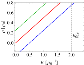
(a) 2 particles

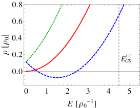
(b) 3 particles

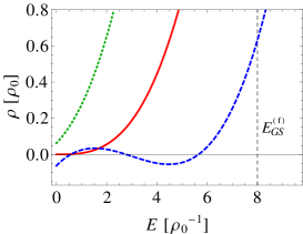
(c) 4 particles

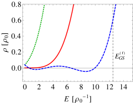
(d) 5 particles

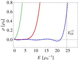
(e) 7 particles

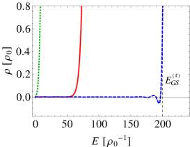
(f) 20 particles

Figure 5: Symmetry-projected DOS without boundary corrections in $D=2$ for bosons (green, dotted) and fermions (blue, dashed) in comparison to the naive volume term (red, solid) for several numbers of particles. The vertical dashed black line shows the particular expected many-body ground state energy $E_{\mathrm{GS}}^{\mathrm{(f)}}$ for fermions (82). Densities $\varrho$ are measured in units of the constant single-particle density $\varrho_{0}$. Energies $E$ are measured in units of its reciprocal $\varrho_{0}^{-1}$

Already here, the symmetry corrections give qualitatively the right picture. With respect to the naive term, the fermionic density is shifted to higher energies, which is according to the expectation of the many-body ground state energy below which effectively no level should appear. Whereas the bosonic density is shifted to lower energies, which accords to the full counting of many-body levels corresponding to shared single-particle energies in contrast to the naive term, where these are counted with a factor of $1/N!$, even if they can not be permuted in $N!$ ways due to identity of some of the single-particle energies.

Figures 5b–5f show the cases of two to twenty particles. In the fermionic case the lower powers in $E$ in the polynomial produce oscillations around the axis $\bar{\varrho}=0$. With increasing particle number these oscillations get smaller in amplitude and larger in number, approximating a zero-valued DOS. The DOS is effectively shifted to higher energies and an energy gap opens that coincides with the expected fermionic ground state energy $E_{\mathrm{GS}}^{\mathrm{(f)}}$ calculated by counting single-particle levels by virtue of the smooth single-particle DOS $\bar{\varrho}_{\mathrm{sp}}(E)$. It is defined by

$$E_{\mathrm{GS}}^{\mathrm{(f)}} :=\int_{-\infty}^{\bar{E}_{\mathrm{F}}}\text{d}E^{\prime}\,\bar{\varrho}_{\mathrm{sp}}(E^{\prime})E^{\prime}\,,$$ (82)

where the Fermi energy $$\bar{E}_{\mathrm{F}}$$ is defined through

$$N =:\int_{-\infty}^{\bar{E}_{\mathrm{F}}}\text{d}E^{\prime}\,\bar{\varrho}_{\mathrm{sp}}(E^{\prime})\,,$$ (83)

but instead of explicitly filling up single-particle energy levels by hand, this time the ground state energy occurs as a consequence out of exchange symmetry incorporated as a modification of the propagator. The corrections from cluster zone propagations are sufficient to automatically reproduce the expected ground state energy. When increasing $N$, the symmetry projected DOS at $E=E_{\mathrm{GS}}^{\mathrm{(f)}}$ is observed to keep moderate values $\bar{\varrho}_{-}(E_{\mathrm{GS}}^{\mathrm{(f)}})\approx\mathcal{O}(1)$ while the naive density at this energy grows exponentially with $N$. In contrast to the fermionic density, the bosonic density does not have these oscillations. There, the polynomial in $E$ has only positive coefficients and the density is effectively shifted to lower energies as expected intuitively.

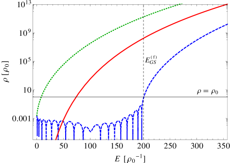
Figure 6: Symmetry-projected DOS in $D=2$ for bosons (green, dotted) and fermions (blue, dashed) in comparison to the naive volume term (red, solid) for $N=20$ particles. Negative values of the fermionic density are plotted as logarithm of its absolute value. The expected many-body ground state energy $E_{\mathrm{GS}}^{\mathrm{(f)}}$ for fermions (82) is represented by the dashed vertical line.

For higher particle numbers a single logarithmic plot suggests itself in order to show at the same time the oscillations that are becoming very small and the strong growth behaviour around and above the ground state energy. Figure 6 shows the smooth part of the density in the case of $N=20$ particles. Again the fermionic energy gap accurately reproduces the ground state energy, indicated by crossing the axis of abscissa. Also in the bosonic case, the corresponding density $\bar{\varrho}_{+}(E)$ apparently keeps moderate values at the expected bosonic ground state energy $E_{\mathrm{GS}}^{\mathrm{(b)}}$ computed in analogue manner to $E_{\mathrm{GS}}^{\mathrm{(f)}}$.

The small values of $\bar{\varrho}_{-}(E)$ for $E\lesssim E_{\mathrm{GS}}^{\mathrm{(f)}}$ result from large cancellations regarding the different terms in the sum (76) with different values of $l$. Therefore the behaviour of the DOS in this regime is very sensitive to numerical errors and all the corrections are needed to reproduce it correctly. In order to illustrate this fact figure 7a shows the deviations one obtains when leaving out contributions.

Another feature of the oscillations around zero up to $E=E_{\mathrm{GS}}^{\mathrm{(f)}}$ is their rigidity with respect to integration in the sense that not only the DOS itself oscillates around zero but do also several integrals of it. Some integrals are shown in figure 7b.

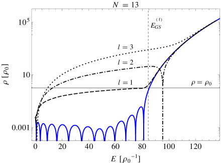
(a) Absolute value of the many-body DOS for $N=13$ fermions. The blue solid curve shows the full expression (73). The black curves correspond to leaving out the contributions $l=1$ (dashed), $l=2$ (dash-dotted) and $l=3$ (dotted).

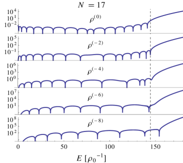
(b) Absolute value of multiple integrals $\varrho^{(-n)}(E)=\int_{0}^{E}\text{d}e_{n}\cdots\int_{0}^{e_{2}}\text{d}e_{1}\,\varrho_{-}(e_{1})$ of the many-body DOS for $N=17$ fermions. Oscillations around zero for energies below $E_{\mathrm{GS}}^{\mathrm{(f)}}$ (vertical dashed line) remain.

Figure 7: Sensitivity (figure 7a) respectively rigidity (figure 7b) of the oscillations of $\bar{\varrho}_{-}(E)$.

The effect of boundary corrections is shown in figure 8. Displayed is the $N=12$ fermionic unconfined level counting function $\mathcal{N}(E)=\int_{0}^{E}\text{d}E^{\prime}\,\bar{\varrho}_{-}(E^{\prime})$ in $2D$ and in addition to that the corresponding confined case (77) for Dirichlet boundary conditions with a geometrical perimeter-to-area-ratio of $\gamma=-\sqrt{\pi}/2$, which is the smallest possible parameter for singly connected billiards since it is the one of a circular billiard. The curve seems to be shifted further to higher energies, enlarging the energy gap. Again the expected ground state energy $E_{\mathrm{GS}}^{(f)}$, this time calculated using the single-particle Weyl expansion with perimeter correction, is reproduced very well. Already for this minimal value of $\gamma$ the deviations from the unconfined case apparently are rather strong. Thus naturally the question arises whether the assumption of locally flat boundaries gives a sufficient description of an actual billiard or additional corrections also lead to rather strong deviations, making the treatment of curvature inevitable. Therefore the exact quantum mechanically solvable levels of a circular billiard have been arranged to non-interacting fermionic many-body levels shown by the green staircase function. The deviation seems again to be effectively a slight shift, smaller than the deviation of the confined from the unconfined case. Not displayed is $E_{\mathrm{GS}}^{(f)}$ including curvature, which in this case coincides with the exact circle levels, in the sense that it lies half way between the first two of them.

\psfrag{xaxis}[bc]{\small$E[\varrho_{0}^{-1}]$}\psfrag{yaxis}[tl][bl][1][180]{\small$\mathcal{N}(E)$}\psfrag{label}[bc]{\small$N=12$}\psfrag{EGS}[bl]{\scriptsize$E_{\mathrm{GS}}^{\mathrm{(f)}}$}\psfrag{EGSi}[bl]{\scriptsize$E_{\mathrm{GS}}^{\mathrm{(f)}}$}\psfrag{N12}[Bl]{\scriptsize$\mathcal{N}=1/2$}\psfrag{N12i}[Bl]{\scriptsize$\mathcal{N}=1/2$}\includegraphics[width=411.93767pt]{Ncirccyl12_bpsfrag.eps}

Figure 8: Level counting function for 12 fermions. The blue dashed curve shows the smooth part without confinement corrections. The black dotted curve includes boundary corrections with a geometrical parameter of $\gamma=-\sqrt{\pi}/2$, which corresponds to a circular billiard. The green staircase (left) shows the exact non-interacting many-body levels of the circular billiard. The red staircase (right) shows the exact levels of a cylindrical billiard with same geometrical parameter. The dash-dotted black curve in the inset shows the smooth part shifted to lower energies corresponding to the shift of $E_{\mathrm{GS}}^{(f)}$ due to curvature.

The additional comparison with exactly computed levels of a billiard with the shape of a cylinder barrel with same $\gamma$-ratio as the circle serving as an example of a $2D$ system without curvature shows good agreement with the smooth part. Note that in this geometry the minimal value of $\gamma$ could be underrun, which is not contradictory since it is not singly connected. The absence of curvature can be seen in the single-particle expansion given by Balian and Bloch [26], where the corresponding correction is proportional to the Euler characteristic $\chi$ of the billiard, which happens to be one for a disk and zero for a cylinder barrel.

An analysis of the $E_{\mathrm{GS}}^{\mathrm{(f)}}$ in $2D$ for the unconfined and confined cases with and without curvature indicate the relative importance of the corresponding contributions in the smooth DOS. The smooth ground state energy involving a Dirichlet type perimeter correction without curvature ($\chi=0$) reads

$$E_{\mathrm{GS}}^{\mathrm{(f)}}(N,\gamma,0)=E_{\mathrm{GS}}^{\mathrm{(f)}}(N,0,0)\,\left(\sqrt{1+a}+\sqrt{a}\right)^{3}\bigl{(}\sqrt{1+a}-\frac{1}{3}\sqrt{a}\bigr{)}\,,\qquad a=\frac{|\gamma|}{\sqrt{\pi N}}\,.$$

The inclusion of the curvature correction $\chi\delta(E)/6$ [26] in the single-particle DOS yields the ground state energy $E_{\mathrm{GS}}^{\mathrm{(f)}}(N,\gamma,\chi)=E_{\mathrm{GS}}^{\mathrm{(f)}}(N-\chi/6,\gamma,0)$. Comparing the correction due to the perimeter ($\chi=0$) with the further correction due to curvature

$$\frac{E_{\mathrm{GS}}^{\mathrm{(f)}}(N,\gamma,\chi)-E_{\mathrm{GS}}^{\mathrm{(f)}}(N,\gamma,0)}{E_{\mathrm{GS}}^{\mathrm{(f)}}(N,\gamma,0)-E_{\mathrm{GS}}^{\mathrm{(f)}}(N,0,0)}=-\frac{\sqrt{\pi}\chi}{8|\gamma|}\sqrt{\frac{1}{N}}+\frac{\chi}{16N}+\mathcal{O}\bigl{(}N^{-\frac{3}{2}}\bigr{)}\,,$$

indicates that curvature contributions in general get strongly suppressed for large particle numbers. Based on this argument, the smooth part of the many-body DOS including curvature in $D=2$ might be approximated by simply shifting the many-body DOS (including perimeter corrections) by $\Delta E=E_{\mathrm{GS}}^{\mathrm{(f)}}(N,\gamma,\chi)-E_{\mathrm{GS}}^{\mathrm{(f)}}(N,\gamma,0)$. The corresponding function is plotted in the inset of figure 8.

\psfrag{xaxis}[Bl]{\scriptsize$E[\varrho_{0}^{-1}]$}\psfrag{yaxis}[tl][bl][1][180]{\scriptsize$\mathcal{N}(E)$}\psfrag{label}[bl]{\small$N=6$}\includegraphics[width=212.47617pt]{Nring6psfrag.eps}

(a)

\psfrag{xaxis}[Bl]{\scriptsize$E[\varrho_{0}^{-1}]$}\psfrag{yaxis}[tl][bl][1][180]{\scriptsize$\mathcal{N}(E)$}\psfrag{label}[bl]{\small$N=9$}\includegraphics[width=212.47617pt]{Nring9psfrag.eps}

(b)

\psfrag{xaxis}[Bl]{\scriptsize$E[\varrho_{0}^{-1}]$}\psfrag{yaxis}[tl][bl][1][180]{\scriptsize$\mathcal{N}(E)$}\psfrag{label}[bl]{\small$N=12$}\includegraphics[width=212.47617pt]{Nring12psfrag.eps}

(c)

\psfrag{xaxis}[Bl]{\scriptsize$E[\varrho_{0}^{-1}]$}\psfrag{yaxis}[tl][bl][1][180]{\scriptsize$\mathcal{N}(E)$}\psfrag{label}[bl]{\small$N=16$}\includegraphics[width=212.47617pt]{Nring16psfrag.eps}

(d)

Figure 9: Level counting function of a ring billiard with $N=6,9,12,16$ fermions. The blue dashed curve shows the (absolute value of the) smooth part with confinement corrections (77) using a geometrical parameter of $\gamma=-\sqrt{3\pi}/2$. The red staircase shows exact non-interacting many-body levels of a ring billiard with the same geometrical parameter which corresponds to a ratio of radii of $2$. The black dotted curve displays the Bethe approximation (105) using the exact ground state energy as input. The horizontal black line corresponds to $\mathcal{N}=1/2$.

It has to be emphasized that the ground state energies reproduced by the smooth densities are defined by smooth counting and do not necessarily have to accurately coincide with the exact many-body ground state energies of actual non-interacting quantum billiards. The exact fermionic ground state levels usually are subject to fluctuations around $E_{\mathrm{GS}}^{\mathrm{(f)}}$ with respect to the particle number $N$, which can be treated with semiclassical methods including corrections from periodic orbits [30]. For rather regular systems possibly featuring degeneracies, these fluctuations in general can become strong and even the average $\langle E_{\mathrm{GS}}^{\mathrm{ex}}(N)\rangle_{N}$ over some window in $N$ can deviate from the smooth prediction $E_{\mathrm{GS}}^{\mathrm{(f)}}(N)$ [30]. A related feature of exact non-interacting many-body spectra are fluctuations of the many-body DOS at low excitation respectively temperature which can also be reproduced as semiclassical shell corrections to the Bethe estimate (105) as shown by Leboeuf et al [31]. Therefore, the smooth part of the symmetry projected DOS (76,77) presented in this work should not be regarded as an estimate for the exact ground state energy of a given system or the behaviour of the actual many-body DOS at energies close to it. Nevertheless, as fluctuations tend to wash out for higher excitations, the correct behaviour is very well reproduced for energies above a critical excitation (which depends on the specific geometry of the system and the particle number $N$). Note that the theoretical prediction of this more universal behaviour does not need any further system specific input than the volume and surface (and a possible non-zero valued Euler characteristic) of the billiard.

Figure 9 shows both, deviations of the smooth prediction near the ground state as manifestation of such fluctuations and the increasingly good agreement for higher energies using the example of a ring billiard with several numbers of fermions. Like the cylindrical billiard, this system has an Euler characteristic of zero and therefore there are no signatures of curvature. Compared are the smooth level counting function $\mathcal{N}(E)$ in the confined case and the exact many-body counting function of a ring billiard with a ratio of $R/r=2$ of outer and inner radius, which corresponds to a geometrical parameter of $\gamma=-\sqrt{3\pi}/2$.

9 Comparison with Known Results

9.1 Smoothing in Weidenmüller Convolution Formula

As Weidenmüller pointed out [21], the symmetry projected part of the exact DOS of a non-interacting system can be constructed as a sum of convolutions of the single-particle DOS with modified energies. The DOS for a non-interacting bosonic (fermionic) system with exact single-particle DOS $\varrho_{\mathrm{sp}}(E)=\sum_{i}\delta(E-\epsilon_{i})$ reads

$$\begin{split}\varrho_{\pm}(E)=&\frac{1}{N!}\sum_{l=1}^{N}(\pm 1)^{N-l}\sum_{\begin{subarray}{c}N_{1},\ldots,N_{l}=1\\ N_{1}\leq\cdots\leq N_{l}\end{subarray}}^{N}\delta_{N,\,\sum N_{\omega}}\;\;c(N_{1},\ldots,N_{l})\Bigl{(}\prod_{\omega=1}^{l}\frac{1}{N_{\omega}}\Bigr{)}\times\\ &\int\text{d}E_{1}\ldots\text{d}E_{l}\;\delta\Bigl{(}E-\sum_{\omega=1}^{l}E_{\omega}\Bigr{)}\;\left[\prod_{\omega=1}^{l}\varrho_{\mathrm{sp}}\Bigl{(}\frac{E_{\omega}}{N_{\omega}}\Bigr{)}\right].\end{split}$$ (84)

The derivation of (84) is on the one hand based on the fact that the non-interacting many-body propagator decomposes into a product of single-particle propagators. On the other hand, this form requires the convolution property

$$\int\text{d}^{D}q^{\prime}\,K^{(\mathrm{sp})}({\bf q}^{\prime\prime},{\bf q}^{\prime};t_{2})K^{(\mathrm{sp})}({\bf q}^{\prime},{\bf q};t_{1})=K^{(\mathrm{sp})}({\bf q}^{\prime\prime},{\bf q};t_{1}+t_{2})$$ (85)

of the single-particle propagator, which is strictly fulfilled for the exact quantum propagator associated with the exact DOS. Inserting the single-particle spectrum directly into (84), one can, in accordance to [21] show that (84) is a formal way to express the construction of many-body levels out of filling up $N$ single-particle levels under the condition that these should be counted correctly. So that no two filled fermionic single particle levels are the same and bosonic states where any of the filled single-particle levels are the same are not undercounted by the factor $1/N!$ but instead fully addressed by counting each of the corresponding possible distributions of single-particle energies among the $N$ particles with the factor of $(\prod_{\omega}N_{\omega}!)/N!$. Here, the $N_{\omega}$ denote the numbers of particles sharing a single-particle level in the questioned many-body state.

The question of whether and, if yes, to what extent formula (84) can be utilized in order to obtain or compare to the smooth part of the symmetry projected DOS can be answered in a twofold way. Naturally this question reduces to the question of how reasonable it is to simply use the smooth part of the single-particle DOS in (84) instead of the exact one.

First, one could regard the smooth part of a spectrum as a convolution with some smearing function. The question is then, if the smoothing of the single-particle DOS in (84) yields the same result as if one would smooth the many-body DOS directly by a similar smoothing procedure. It turns out that this can be answered positively if the function used for smoothing obeys two conditions. Let $\delta_{\alpha}(x)$ denote the smoothing function with a continuous parameter $\alpha$ describing its sharpness and $\int_{-\infty}^{\infty}\text{d}x\,\delta_{\alpha}(x)=1$. If this function fulfils

$$\delta_{c\alpha}(x)=\frac{1}{c}\delta_{\alpha}\left(\frac{x}{c}\right)\,,\qquad c>0\,,$$ (86)

$$\int_{-\infty}^{\infty}\text{d}y\,\delta_{\alpha}(x-y)\delta_{\beta}(y)=\delta_{\alpha+\beta}(x)\,,$$ (87)

then the replacement of the single-particle DOS $\varrho_{\mathrm{sp}}$ by its convolution with $\delta_{\alpha}$ yields the same as convolving the many-body DOS $\varrho_{\pm}$ with $\delta_{N\alpha}$. If the function $\delta_{\alpha}$ perceived as a distribution had a finite mean value and variance, then (86) implies that $\alpha$ is proportional to the standard deviation. But then this would contradict the second condition (87) as the variance in general is additive under convolution instead of the standard deviation. This shows that a proper smoothing function in this context should not have a finite standard deviation. Nevertheless, there is a distribution without standard deviation fulfilling the requirements at hand, namely the Cauchy distribution

$$\delta_{\alpha}(x)=\frac{\alpha}{\pi(\alpha^{2}+x^{2})}\,.$$ (88)

The second way to address the question is to replace the exact single-particle DOS in (84) by the smooth part $\bar{\varrho}_{\mathrm{sp}}$ defined by the Weyl expansion up to a specified order. In the cases of restricting to the volume term and considering also the first boundary correction in $\bar{\varrho}_{\mathrm{sp}}$ the corresponding integrals over single-particle energies are carried out successively yielding a solvable recursion relation. A and C show these calculations with the outcome that this procedure yields the same result for $\bar{\varrho}_{\pm}(E)$ as the investigation of the propagation in cluster zones (76, 77).

The reason why both procedures give the same result lies in the requirement (85). For the exact quantum propagator the fulfilment of it is obvious. In the unconfined case the exact propagator is replaced by the free propagator, which also obeys the convolution property, but only if the intermediate coordinates ${\bf q}^{\prime}$ are integrated over full space $\mathbb{R}^{D}$ and not only the interior $\Omega$ of the billiard. Recalling the derivation of (76), this corresponds exactly to the extension of the integration limits for all intermediate coordinates $q_{2},\ldots,q_{n}$ in (60) allowing the evaluation of the integral as multidimensional Gaussian. Thus the assumption of infinite distance to the boundary in the analysis of cluster propagations in combination with the usage of the free propagator actually preserves the convolution property (85).

In the confined case the free propagator is modified by a reflection term

$$K^{(\mathrm{sp})}_{0}({\bf q}^{\prime},{\bf q};t)\rightarrow K^{(\mathrm{sp})}_{0}({\bf q}^{\prime},{\bf q};t)\pm K^{(\mathrm{sp})}_{0}(R{\bf q}^{\prime},{\bf q};t)\,,$$ (89)

where $R$ denotes the reflection with respect to the boundary regarded as locally flat and $\pm$ refers to Neumann respectively Dirichlet conditions. This replacement yields the Weyl expansion including the surface correction. The analysis in B shows that the so constructed propagator in combination with the assumption of local flatness of the boundary also exhibits the convolution property (85). This shows the equivalence of the computation $\bar{\varrho}_{\pm}(E)$ in the confined case (77) via the convolution of single-particle Weyl expansions up to the first boundary correction and the computation by investigation of the propagation in cluster zones including reflections on the boundary assumed as locally flat.

This equivalence gives rise to the question whether it is possible to relate corrections from propagation in cluster zones to the correction of delta peaks that is inherent to the exact convolution formula (84) of Weidenmüller. And indeed one can relate each cluster zone correction to the correction of delta peaks for total energies. The corrected total energy is the energy that is a partition of single-particle energies just the way the cluster zone corresponds to a partition of all particles into clusters. The cluster zone correction is associated to the correction of the total energy that is built of single-particle energies, where all particles in a cluster share the same energy. But of course it is doing it in a smooth manner, meaning it produces a smooth correction to the DOS corresponding to a smooth version of the density constructed out of such many-body energies with correct prefactor.

9.2 Connection to Bethe’s Estimate in Fermionic Systems

This section is dedicated to the connection between the expressions presented in this work and the celebrated Bethe approximation to the many-body DOS. As the latter results as a saddle point approximation of an integral representation of the DOS obtained by general quantum statistical methods for non-interacting fermionic systems, the link between both is the equivalence of the smooth part of the DOS (76,77) and the standard statistical formulation in terms of the single-particle DOS. This connection will be drawn by the usage of the technique of generating functions as the easiest to handle statistical object associated with the DOS is the grand canonical partition function $\mathcal{Z}^{\mathrm{GC}}(z,\beta)$ which itself is the generating function of the canonical partition functions for $N$ particles

$$\mathcal{Z}^{\mathrm{C}}(N,\beta)=\frac{1}{N!}\frac{\text{d}^{N}}{\text{d}z^{N}}\mathcal{Z}^{\mathrm{GC}}(z,\beta)\Bigr{\rvert}_{z=0}\,.$$ (90)

The essential step in order to find the generating function for the DOS (77)

$$G_{\pm}(z,E) =\sum_{N=0}^{\infty}\bar{\varrho}_{\pm}(N,E)z^{N},$$ (91)

$$\Leftrightarrow\bar{\varrho}_{\pm}(N,E) =\frac{1}{N!}\frac{\text{d}^{N}}{\text{d}z^{N}}G(z,E)\Bigr{\rvert}_{z=0}\,,$$ (92)

is to represent the difficult to handle combinatorial numbers $C_{l},C_{l,l_{\text{V}}}$ (73), (77) in terms of their generating functions. In order to ease notation, the abbreviations $\mu=\frac{D}{2}+1$ and $\nu=\frac{D-1}{2}+1$ are used.

$$C_{l}^{(N)}=\frac{1}{N!}\frac{\text{d}^{N}}{\text{d}z^{N}}\left.\biggl{(}\sum_{n=0}^{\infty}\frac{z^{n}}{n^{\mu}}\biggr{)}^{l}\right|_{z=0}=\frac{1}{N!}\frac{\text{d}^{N}}{\text{d}z^{N}}\left.\left(\mathrm{Li}_{\mu}(z)\right)^{l}\right|_{z=0}$$ (93)

and similarly

$$C_{l,l_{\text{V}}}^{(N)} =\frac{1}{N!}\frac{\text{d}^{N}}{\text{d}z^{N}}\left.\left[\biggl{(}\sum_{n=0}^{\infty}\frac{z^{n}}{n^{\mu}}\biggr{)}^{l_{\text{V}}}\biggl{(}\sum_{n=0}^{\infty}\frac{z^{n}}{n^{\nu}}\biggr{)}^{l-l_{\text{V}}}\right]\right|_{z=0}$$

$$=\frac{1}{N!}\frac{\text{d}^{N}}{\text{d}z^{N}}\left[\left(\mathrm{Li}_{\mu}(z)\right)^{l_{\text{V}}}\left(\mathrm{Li}_{\nu}(z)\right)^{l-l_{\text{V}}}\right]\Biggr{\rvert}_{z=0}\,.$$ (94)

These relations can be seen by factoring out the powers of the sums in parentheses and recognizing that the $N$-th power of $z$ in the product must be built of $l$ factors $z^{n_{i}},i=1,\ldots,l$ with $\sum_{i}n_{i}=N$. Thus each such combination corresponds to a particular partition of $N$ into $l$ parts $n_{1}+\cdots+n_{l}$. The correct coefficients are then created as products of the parts $n_{i}^{\mu/\nu}$ appearing as denominators in the sums over $n$. The generating functions can also be built constructively which will be shown exemplarily for the unconfined case. The confined case can be treated similarly. For this calculation the form of $C_{l}^{(N)}$ expressed as sum over distinct partitions instead of ordered tuples will be used. Note that $C_{l}^{(N)}$ should be understood to be zero for all $l>N$. The starting point is to calculate constructively the generating function of $C_{l}^{(N)}/l!$ which is

$$g_{l}(z):=\frac{1}{l!}\sum_{N=0}^{\infty}C_{l}^{(N)}z^{N} =\sum_{N=0}^{\infty}\,\sum_{{\begin{subarray}{c}N_{1}\leq\ldots\leq N_{l}=1\\ \sum N_{\omega}=N\end{subarray}}}^{N}\biggl{(}\prod_{n=1}^{\infty}\frac{1}{m_{n}!}\biggr{)}\biggl{(}\prod_{\omega=1}^{l}\frac{1}{N_{\omega}}\biggr{)}^{\mu}z^{N}$$

$$=\sum_{\begin{subarray}{c}{\bf m}\in\mathbb{N}_{0}^{\mathbb{N}}\\ \sum m_{n}=l\end{subarray}}\prod_{n=1}^{\infty}\frac{z^{n\,m_{n}}}{m_{n}!\,n^{\mu\,m_{n}}}\,,$$ (95)

where the sum over all possible distinct partitions is expressed as sum over all multiplicities $m_{n}$ with which the part sizes $n=1,2,\ldots$ appear. Given a fixed value of $l$ corresponds to the restriction $\sum m_{n}=l$ in the sum. This restriction is dropped by constructing a further generating function of (95), this time with respect to $l$.

$$\sum_{l=1}^{\infty}g_{l}(z)y^{l}=\prod_{n=1}^{\infty}\left[\sum_{m=0}^{\infty}\frac{1}{m!}\left(\frac{z^{n}y}{n^{\mu}}\right)^{m}\right]=\prod_{n=1}^{\infty}\exp\left(\frac{z^{n}y}{n^{\mu}}\right)=\exp\left[y\mathrm{Li}_{\mu}(z)\right]\,.$$ (96)

Making use of this secondary generating function shows that

$$g_{l}(z)=\frac{1}{l!}\frac{\text{d}^{l}}{\text{d}y^{l}}\exp\left[y\mathrm{Li}_{\mu}(z)\right]\Bigr{\rvert}_{y=0}=\frac{1}{l!}\left[\mathrm{Li}_{\mu}(z)\right]^{l}\,.$$ (97)

Note that because of $\mathrm{Li}_{\mu}(z)=\mathcal{O}(z)$ as $z\rightarrow 0$, indeed the $C_{l}$ vanish for $l>N$.

From here, the confined case will explicitly be treated, including the unconfined case as $\gamma=0$. Using (9.2) in (77) gives

$$G_{\pm}(z,E)=\varrho_{0}\sum_{l=0}^{\infty}(\pm 1)^{l}\sum_{\begin{subarray}{c}l_{\text{V}},l_{\text{S}}=0\\ \sum l_{i}=l\end{subarray}}^{l}\frac{[\mathrm{Li}_{\mu}(\pm z)]^{l_{\text{V}}}[\mathrm{Li}_{\nu}(\pm z)]^{l_{\text{S}}}}{l_{\text{V}}!\;l_{\text{S}}!}\gamma^{l_{\text{S}}}\frac{(\varrho_{0}E)^{\lambda-1}}{\Gamma\left(\lambda\right)}\theta(E)$$ (98)

with the abbreviated exponent $\lambda=l_{\text{V}}D/2+l_{\text{S}}(D-1)/2$ and $\mu=D/2+1$, $\nu=(D-1)/2+1$ as before. The upper limit of the sum over $l$ has been raised from $N$ to infinity which is no problem since the $N$-th derivative at $z=0$ is not affected by terms with $l>N$. Applying Laplace transformation switches from energy domain to the domain of inverse temperature and allows for exact summation of $l_{\text{V}}$ and $l_{\text{S}}$.

$$G_{\pm}(z,E) =\mathcal{L}^{-1}_{\beta}\bigg{[}\sum_{l_{\text{V}},l_{\text{S}}=0}^{\infty}\frac{[\pm\mathrm{Li}_{\mu}(\pm z)]^{l_{\text{V}}}[\pm\mathrm{Li}_{\nu}(\pm z)]^{l_{\text{S}}}}{l_{\text{V}}!\;l_{\text{S}}!}\gamma^{l_{\text{S}}}\Bigl{(}\frac{\varrho_{0}}{\beta}\Bigr{)}^{\lambda}\biggr{]}(E)$$

$$=\mathcal{L}^{-1}_{\beta}\left[\exp\biggl{(}\pm\Bigl{(}\frac{\varrho_{0}}{\beta}\Bigr{)}^{\frac{D}{2}}\mathrm{Li}_{\mu}(\pm z)\pm\gamma\Bigl{(}\frac{\varrho_{0}}{\beta}\Bigr{)}^{\frac{D-1}{2}}\mathrm{Li}_{\nu}(\pm z)\biggr{)}\right](E)\,.$$ (99)

In the case of $D=1$, the replacement rule (80) is already accounted for in (9.2). Note that the bilateral definition of Laplace transform is used, which simply yields the Heaviside step function $\theta(E)$ after taking the inverse Laplace transform.

The result (9.2) is equivalent to the grand canonical potential one obtains by standard statistical methods. In general, the grand canonical potential of a non-interacting quantum system of identical particles can be expressed in terms of the single-particle DOS as

$$\ln\mathcal{Z}^{\mathrm{GC}}_{\pm}(z,\beta)=\mp\int\text{d}E\,\varrho_{\mathrm{sp}}(E)\ln(1\mp z\mathrm{e}^{-\beta E})\,,$$ (100)

where the upper sign corresponds to bosonic symmetry ($z$ has to be small enough in modulus to keep the argument of the logarithm inside the unit disk around $1$) and the lower one corresponds to fermionic statistics. If the single-particle DOS is taken as its smooth part built as a sum of smooth functions of the form

$$\varrho_{i}(E)=\varrho_{0}\gamma_{i}\frac{(\varrho_{0}E)^{\nu_{i}-1}}{\Gamma(\nu_{i})}\theta(E)\,,$$ (101)

each of the summands yields an additive contribution

$$\ln\mathcal{Z}^{\mathrm{GC}}_{\pm,i}(z,\beta) =\pm\gamma_{i}\varrho_{0}^{\nu_{i}}\sum_{k=1}^{\infty}\frac{(\pm z)^{k}}{k}\,\frac{1}{\Gamma(\nu_{i})}\int_{0}^{\infty}\text{d}E\,E^{\nu_{i}-1}\mathrm{e}^{-k\beta E}$$

$$=\pm\gamma_{i}\Bigl{(}\frac{\varrho_{0}}{\beta}\Bigr{)}^{\nu_{i}}\sum_{k=1}^{\infty}\frac{(\pm z)^{k}}{k^{\nu_{i}+1}}$$

$$=\pm\gamma_{i}\Bigl{(}\frac{\varrho_{0}}{\beta}\Bigr{)}^{\nu_{i}}\mathrm{Li}_{\nu_{i}+1}(\pm z)\,,$$ (102)

which shows the equivalence to (9.2) due to $\mathcal{Z}^{\mathrm{GC}}=\mathcal{L}[G]$ when taking the appropriate single-particle DOS with $\gamma_{1}=1,\nu_{1}=D/2$ in the first term and $\gamma_{2}=\gamma,\nu_{2}=(D-1)/2$ in the second one. The derivation of (100) involves the replacement

$$\sum_{i}f(E_{i})\rightarrow\int\text{d}E\,\varrho_{\mathrm{sp}}(E)f(E)$$ (103)

of the sum over single-particle eigenenergies, which are assumed to be discrete in the first place. Simply taking the smooth part of the single-particle DOS instead is therefore closely related to taking the smooth part in the convolution formula (84) by Weidenmüller, which we showed to be equivalent to the actual smooth part of the many-body density obtained with the geometrical approach.

For practical reasons it should be mentioned that in the unconfined case $\gamma=0$ in $D=2$, the inverse Laplace transform in (9.2) can be done explicitly to get

$$G_{\pm}^{(D=2,\gamma=0)}(z,E)=\varrho_{0}\sqrt{\pm\frac{\mathrm{Li}_{2}(\pm z)}{\varrho_{0}E}}\;\mathrm{I}_{1}\!\left(2\sqrt{\pm\mathrm{Li}_{2}(\pm z)\varrho_{0}E}\right)\,,$$ (104)

which could also be seen directly from (98) after recognizing the power series of the modified Bessel function $\mathrm{I}_{1}(x)$ with the two factorials $l_{\text{V}}!$ and $\Gamma(\lambda)=(l_{\text{V}}-1)!$ in the denominator ($l_{\text{S}}=0$).

The Bethe approximation [13] of the non-interacting fermionic many-body DOS is based on the general statistical relation (100) and reads

$$\bar{\varrho}_{\mathrm{B}}(Q)=\frac{1}{\sqrt{48}\,Q}\exp\left(\sqrt{\frac{2\pi^{2}}{3}\bar{\varrho}\,Q}\right)\,,$$ (105)

where $Q=E-E_{\mathrm{GS}}>0$ is the excitation energy above the many-body ground state energy (82) and $\bar{\varrho}=\bar{\varrho}_{\mathrm{sp}}(E_{\mathrm{F}})$ is the single-particle DOS at the Fermi energy (83). It results from a low temperature expansion and a simultaneous complex saddle point approximation in two integrals. The first one being the Bromwich integral achieving the inverse Laplace transform of $\mathcal{Z}^{\mathrm{GC}}$ and the second one being a closed complex contour integral representing its $N$-th derivative with respect to $z$. The low temperature expansion limits the validity of (105) to low excitation energies $Q\lesssim E_{\mathrm{F}}$ (range increases with $N$) whereas the defect produced by the saddle point approximations becomes noticeable when approaching the ground state energy $Q\lesssim\bar{\varrho}^{-1}$ and culminates in the divergence at $Q=0$.
Despite the fact that (105) is valid in general and is not depending on the specific form of the single-particle density, it shall be sketched here how to obtain it explicitly for the unconfined case using expression (9.2) respectively (9.2), since the explicit expressions can be of use investigating possible extensions to (105) that are not general. Expressing the inverse Laplace transform and derivation with respect to $z$ as integrals, the smooth part of the fermionic many-body DOS for $N$ particles in a $D$-dimensional billiard ($\nu=D/2$) without confinement corrections reads

$$\bar{\varrho}_{-}(N,E)=\left(\frac{1}{2\pi i}\right)^{2}\int_{\mathrlap{\Gamma_{\beta}}}\;\text{d}\beta\int_{\mathrlap{\Gamma_{\alpha}}}\;\text{d}\alpha\;\exp\left[\beta E-\alpha N-\beta^{-\nu}\mathrm{Li}_{\nu+1}(-\mathrm{e}^{\alpha})\right]\,,$$ (106)

where $\mathrm{e}^{\alpha}:=z$ and energies are measured in units of $\varrho_{0}$. The contours are $\Gamma_{\beta}:(\epsilon-i\infty,\epsilon+i\infty)$ with $\epsilon\rightarrow 0^{+}$ because of the essential singularity at $\beta=0$ and $\Gamma_{\alpha}:(a-i\pi,a+i\pi)$ with real $a\leq 0$, corresponding to a closed counterclockwise circular contour for $z$ inside the unit circle, chosen because of the branch cut $z\in(-\infty,-1]$ of $\mathrm{Li}_{\nu+1}(-z)$. Applying saddle point approximation in both integrals will yield a saddle point that has a large positive real value in $\alpha$ in the requested regime. Therefore the contour for $z=\mathrm{e}^{\alpha}$ has to be thought of to be deformed outside the unit circle enclosing part of the branch cut. Nevertheless, only the behaviour in the vicinity of the saddle point shall be regarded, dropping the exact form of integration contours and neglecting the integration along the branch cut, allowing for an asymptotic expansion of the polylogarithm for large arguments $|z|\gg 1$ or $\Re(\alpha)\gg 1$. The way to proceed is the following. First $\alpha$ is considered to have a large real part. From the consequent approximation the saddle point will be found to fulfil this statement, justifying the assumption afterwards in a self-consistent manner. The asymptotic expansion of $\mathrm{Li}_{\nu+1}$ leaves the exponent in (106) - which has the statistical interpretation of entropy - as

$$S(\beta,\alpha)\approx\beta E-\alpha N+\beta^{-\nu}\left(\frac{\alpha^{\nu+1}}{\Gamma(\nu+2)}+\frac{\pi^{2}}{6}\,\frac{\alpha^{\nu-1}}{\Gamma(\nu)}\right)\,.$$ (107)

The saddle point equations are

$$N =\frac{\mu^{\nu}}{\Gamma(\nu+1)}+\frac{\pi^{2}}{6\beta^{2}}\,\frac{\mu^{\nu-2}}{\Gamma(\nu-1)}\,,$$ (108)

$$E =\frac{\nu\,\mu^{\nu+1}}{\Gamma(\nu+2)}+\frac{\pi^{2}}{6\beta^{2}}\,\frac{\nu\,\mu^{\nu-1}}{\Gamma(\nu)}$$ (109)

at the saddle point values of $\beta$ and $\mu=\alpha/\beta$, statistically interpreted as inverse temperature and chemical potential. The right hand sides of (108) and (109) match the statistical definitions of mean particle number $\langle N\rangle$ and mean energy $\langle E\rangle$ in the grand canonical formalism. Thus the saddle point values of $\beta$ and $\mu$ fix the ensemble averages of energy and number of particles to the given values $\langle N\rangle=N$ and $\langle E\rangle=E$. For further computation, it is convenient to express the equations in terms of the following quantities.

$$\varrho(\mu) =\frac{\mu^{\nu-1}}{\Gamma(\nu)}\,, \qquad\varrho^{\prime}(\mu) =\frac{\mu^{\nu-2}}{\Gamma(\nu-1)}\,,$$ (110)

$$\mathcal{N}(\mu) =\frac{\mu^{\nu}}{\Gamma(\nu+1)}\,, \mathcal{E}(\mu) =\frac{\nu\,\mu^{\nu+1}}{\Gamma(\nu+2)}\,,$$

with the level counting function $\mathcal{N}(\mu)=\int_{-\infty}^{\mu}\text{d}E\,\varrho(E)$ and the total many-body energy $\mathcal{E}(\mu)=\int_{-\infty}^{\mu}\text{d}E\,E\varrho(E)$ up to $E=\mu$. $\bar{\varrho}_{\mathrm{sp}}$ has been abbreviated to $\varrho$ in order to ease notation. The saddle point equations then read

$$N =\mathcal{N}(\mu)+\frac{\pi^{2}}{6\beta^{2}}\,\varrho^{\prime}(\mu)\,,$$ (111)

$$E =\mathcal{E}(\mu)+\frac{\pi^{2}}{6\beta^{2}}\,(\mu\varrho(\mu))^{\prime}\,,$$ (112)

matching the Sommerfeld expansions up to the first term. Since $\mu\approx E_{\mathrm{F}}$ at the saddle point in the requested regime, one can expand

$$\mathcal{N}(\mu) \approx\underbrace{\mathcal{N}(E_{\mathrm{F}})}_{=N}+\varrho(\mu)\,(\mu-E_{\mathrm{F}})\,,$$ (113)

$$\Rightarrow\quad\mathcal{E}(\mu) \approx\mathcal{E}(E_{\mathrm{F}})+\mu\varrho(\mu)\,(\mu-E_{\mathrm{F}})\stackrel{{\scriptstyle(\ref{eq SPE N 2})}}{{\approx}}E_{\text{GS}}-\frac{\pi^{2}}{6\beta^{2}}\,\mu\varrho^{\prime}(\mu)\,,$$ (114)

leading to

$$E-E_{\text{GS}}\approx\frac{\pi^{2}}{6\beta^{2}}\,\varrho(\mu)\,.$$ (115)

The entropy at the saddle point

$$S=\Bigl{(}1+\frac{1}{\nu}\Bigr{)}\beta E-\alpha N$$ (116)

computes to

$$\frac{1}{\beta}\,S =(\nu+1)\frac{\mu^{\nu+1}}{\Gamma(\nu+2)}+(\nu+1)\frac{\pi^{2}}{6\beta^{2}}\,\frac{\mu^{\nu-1}}{\Gamma(\nu)}-\frac{\mu^{\nu+1}}{\Gamma(\nu+1)}-\frac{\pi^{2}}{6\beta^{2}}\,\frac{\mu^{\nu-1}}{\Gamma(\nu-1)}\,,$$

$$\Rightarrow S =2\frac{\pi^{2}}{6\beta^{2}}\,\frac{\mu^{\nu-1}}{\Gamma(\nu)}=2\frac{\pi^{2}}{6\beta^{2}}\,\varrho(\mu)\beta=2\beta(E-E_{\text{GS}})\,.$$ (117)

And by exploiting (115) one finds $S=\sqrt{\frac{2\pi^{2}}{3}\,\bar{\varrho}\,Q}$. What is left is the computation of the determinant of second derivatives of $S$ with respect to $\beta$ and $\alpha$

$$|\det S^{\prime\prime}|=\left|\frac{\partial(\langle N\rangle,\langle E\rangle)}{\partial(\alpha,\beta)}\right|=\frac{1}{\beta}\left|\frac{\partial(\langle N\rangle,\langle E\rangle)}{\partial(\mu,\beta)}\right|\,.$$ (118)

After neglecting terms that are sub-dominant in the low temperature limit like $\frac{1}{\beta}\,\varrho^{(n+1)}(\mu)\ll\varrho^{(n)}(\mu)$, one finds

$$|\det S^{\prime\prime}|\approx\frac{\pi^{2}}{3\beta^{4}}[\varrho(\mu)]^{2}=\frac{12}{\pi^{2}}(E-E_{\text{GS}})^{2}\,.$$ (119)

Collecting everything and accounting for a minus sign due to the directions of the integration paths in the saddle point finally gives the Bethe approximation

$$\bar{\varrho}_{-}(N,E)\approx\frac{1}{\sqrt{48}\,(E-E_{\text{GS}})}\exp\left(\sqrt{\frac{2\pi^{2}}{3}\bar{\varrho}\cdot(E-E_{\text{GS}})}\right)\,,$$ (120)

with the ground state energy $E_{\text{GS}}=\nu[\Gamma(\nu+1)N]^{1+\frac{1}{\nu}}/\Gamma(\nu+2)$ which matches the definition of smoothly counted ground state energy $E_{\text{GS}}^{\text{(f)}}$ (82). What is left is to show the consistency of $\alpha\gg 1$ at the saddle point. From (115) one obtains

$$\alpha\approx\frac{\pi\mu\varrho(\mu)}{\sqrt{6\varrho(\mu)Q}}=\frac{\pi\nu\mathcal{N}(\mu)}{\sqrt{6\bar{\varrho}\,Q}}\,.$$ (121)

Together with $\mathcal{N}(\mu)=N-\frac{\pi^{2}}{6\alpha^{2}}\nu(\nu-1)\mathcal{N}(\mu)$ from (113), $\alpha$ computes to

$$\alpha\approx\frac{\pi\nu N}{\sqrt{6\bar{\varrho}\,Q}}-\frac{\pi^{2}}{6}\,\frac{\nu(\nu-1)}{\alpha}\,.$$ (122)

Thus in the regime of low excitation energies and high numbers of particles, the assumption is self-consistently justified with

$$\alpha\approx\frac{\pi\nu N}{\sqrt{6\bar{\varrho}\,Q}}+\mathcal{O}\Bigl{(}\frac{\sqrt{\bar{\varrho}Q}}{N}\Bigr{)}\,.$$ (123)

Figure 10: Symmetry-projected DOS without boundary corrections in $D=2$ for $N=3,5,10$ and $28$ fermions (blue, solid) in comparison with the Bethe approximation (black, dotted) and the finite-size corrected improved form (124) (brown, dashed). Densities are measured in units of $\varrho_{0}$ (74). The grey line indicates $\varrho(E)=\varrho_{0}$.

Figure 10 compares the Bethe approximation with the unconfined densities in two dimensions for different numbers of particles. The approximation gets better for increasing $N$ and decreasing $Q$ (down to $Q\sim\varrho_{0}^{-1}$). The displayed energy window scales with $N^{2}$. Thus the similar looking plots for $N\gtrsim 10$ show that the range of excitation energy in which $\bar{\varrho}_{\mathrm{B}}(Q)$ gives reasonable results roughly scales also with $N^{2}$ as indicated by (123). Note that the Bethe approximation needs the information about the particular many-body ground state energy as additional input (which has here been taken as $E_{\mathrm{GS}}^{\mathrm{(f)}}$) whereas the smooth part of the unconfined symmetry-projected density does not but instead automatically provides it. In addition to $\bar{\varrho}_{\mathrm{B}}(Q)$, also an improved form including finite-$N$ corrections,

$$\bar{\varrho}_{\text{F}}(N,Q)=\bar{\varrho}_{\mathrm{B}}(Q)\;\exp\left[\biggl{(}\frac{1}{2}-\frac{\sqrt{6\bar{\varrho}\,Q}}{\pi}\biggr{)}\exp\biggl{(}-\frac{\pi N}{\sqrt{6\bar{\varrho}\,Q}}\biggr{)}\right]\,,$$ (124)

is plotted. Equation (124) can be found in number theoretical context [32] as approximation to the smooth part $\bar{p}_{N}(n)$ of the number of possible partitions of an integer $n$ where all parts are restricted to a maximum size $N$. This function is equivalent to the non-interacting many-body DOS for an equidistant single-particle spectrum which makes the connection between number theory and many-body physics in this context. There is also a generalization [22] of (124) obtained by saddle point approximation in the statistical approach similar to the derivation of $\bar{\varrho}_{\mathrm{B}}(Q)$ but including a correction $\sim\mathrm{e}^{-\alpha}$ to the asymptotic expansion of the polylogarithm (107) in (106) for small $\Re(\alpha)$. The resulting expressions are generalized for single-particle DOS of arbitrary power $\bar{\varrho}_{\mathrm{sp}}(E)\sim E^{\nu-1}$.

10 Conclusion and Outlook

In this paper we have made explicit the essential geometrical content behind the smooth part of the density of states in systems of non-interacting particles. We have shown that both the functional form of the level density and the ground state energy are consequence of a large cancellation effect between contributions polynomial in the energy related with manifolds in configuration space which are invariant under the group of permutations. Our results cover the whole regime of energies and are valid for any number of particles.

The main message of our work is the rigorous construction of the connection between polynomial contributions to the density of states and the measures and dimensions of manifolds in the classical phase space which are invariant under particular permutations of the particles. Moreover, by means of algebraic manipulations we have transformed our expression in a way that explicitly shows its equivalence with several known but previously unconnected results. In particular, by re-expressing the sum over cluster zones in terms of generating functions, we have established its equivalence with the thermodynamic formalism leading to the celebrated Bethe estimate for the level density in fermionic systems.

The geometry of invariant manifolds presented here is a purely kinematic concept independent on any particular dynamics, and although we have used it to fully construct the level density for non-interacting systems (76,77), we expect that it plays also a fundamental role when interparticle interactions are present. In order to apply our formalism in this more general scenario, the key step is to relax the condition expressed by (47) which makes explicit the assumption of non-interacting particles. In the case of interacting particles, however, the key concept remains the same: the smooth part of the density of states does not require the solution of the problem including both interactions and confinement simultaneously. Symmetry effects on the Weyl expansion for interacting systems are encoded in unconfined (but interacting) propagation around cluster zones.

In order to keep the problem tractable, well controlled approximations for the unconfined (but still interacting) many-body propagator are necessary, and the first task to extend our methods into interacting systems is to check the physical picture one gets when a certain approximation for the unconfined propagator is used around the cluster zones. One possible scenario where this program can be carried on is when we treat the interactions in eikonal approximation, freezing the interactions between sets of particles in different cluster zones. This and other possible approximations will be reported in a future publication.

Appendix A Calculation via Convolution Formula - unconfined case

The single-particle Weyl volume term reads

$$\bar{\varrho}_{\mathrm{sp}}(E)=\left(\frac{m}{2\pi\hbar^{2}}\right)^{\frac{D}{2}}\;V_{D}\;\frac{E^{\frac{D}{2}-1}}{\Gamma\left(\frac{D}{2}\right)}\,\theta(E)\equiv a\;E^{\frac{D}{2}-1}\,\theta(E)\,.$$ (125)

Using (84) yields the sum

$$\bar{\varrho}_{\mathrm{conv},\pm}(E)=\frac{1}{N!}\sum_{l=1}^{N}(\pm 1)^{N-l}\sum_{\begin{subarray}{c}N_{1},\ldots,N_{l}=1\\ N_{1}\leq\cdots\leq N_{l}\end{subarray}}^{N}\delta_{N,\,\sum N_{\omega}}\;\;c(N_{1},\ldots,N_{l})\Bigl{(}\prod_{\omega=1}^{l}\frac{1}{N_{\omega}}\Bigr{)}\;\mathcal{C}(E)$$ (126)

of convolutions $\mathcal{C}(E)$ of the form

$$\mathcal{C}(E)= \int\text{d}E_{1}\ldots\text{d}E_{l}\,\left[\prod_{\omega=1}^{l}\bar{\varrho}_{\mathrm{sp}}\Bigl{(}\frac{E_{\omega}}{N_{\omega}}\Bigr{)}\right]\,\delta\Bigl{(}E-\sum_{\omega=1}^{l}E_{\omega}\Bigr{)}=a^{l}\frac{\partial}{\partial E}\mathcal{I}(E)\,,$$ (127)

$$\mathcal{I}(E):= \Bigl{(}\prod_{\omega=1}^{l}\frac{1}{N_{\omega}}\Bigr{)}^{\frac{D}{2}-1}\;\int_{0}^{\infty}\text{d}E_{1}\ldots\text{d}E_{l}\;\prod_{\omega=1}^{l}E_{\omega}^{\frac{D}{2}-1}\;\theta\Bigl{(}E-\sum_{\omega=1}^{l}E_{\omega}\Bigr{)}\,.$$ (128)

$\mathcal{I}(E)$ can be calculated by successively performing the integrals of single-particle energies $E_{\omega}$ and solving an emerging recursion relation. It is convenient to write $r=D/2-1$ and define a new variable for the energy to be distributed among the first $n$ particles for every $n$

$$e_{n}=E-\sum_{\omega=n+1}^{l}E_{\omega},\qquad n=0,\ldots,l-1\,.$$ (129)

The first step in the integral of $\mathcal{I}(E)$ is then

$$\int_{0}^{\infty}\text{d}E_{1}E_{1}^{r}\theta(e_{1}-E_{1}) =\frac{1}{r+1}e_{1}^{r+1}\theta(e_{1})=\frac{1}{r+1}(e_{2}-E_{2})^{r+1}\theta(e_{2}-E_{2})\,.$$ (130)

The next integral over $E_{2}$ is of the form

$$\int_{0}^{c}\text{d}x\;x^{r}\,(c-x)^{s}\theta(c)=c^{s+r+1}\frac{\Gamma(1+r)\Gamma(1+s)}{\Gamma(2+r+s)}\theta(c)\,,$$ (131)

with $c=e_{2}=e_{3}-E_{3}$. Therefore, also the third integral and all others are of this form. Let $A_{n}$ be the total prefactor and $s_{n}$ the exponent $s$ in (131) appearing in the $n$-th integral step. Then one gets the recurrence relation

$$A_{n+1} =A_{n}\frac{\Gamma(1+r)\Gamma(1+s_{n})}{\Gamma(2+r+s_{n})}\,, \quad A_{1} =1\,,$$ (132)

$$s_{n+1} =r+s_{n}+1\,, s_{1} =0\,.$$

The convolution (127) is then expressed as

$$\mathcal{C}(E)=\Bigl{(}\prod_{\omega=1}^{l}\frac{1}{N_{\omega}}\Bigr{)}^{\frac{D}{2}-1}\,a^{l}\,A_{l+1}\,s_{l+1}\,E^{s_{l+1}-1}\theta(E)\,.$$ (133)

The solution of the recurrence reinserting $r=D/2-1$ is

$$A_{n+1}=\frac{\left[\Gamma\left(\frac{D}{2}\right)\right]^{n}}{\Gamma\left(\frac{nD}{2}+1\right)}\,,\quad s_{n+1}=\frac{nD}{2}\,,\qquad n\geq 0\,.$$ (134)

Using the the original expression for $a$ one gets the final result

$$\begin{split}\bar{\varrho}_{\mathrm{conv},\pm}(E)=&\frac{1}{N!}\sum_{l=1}^{N}(\pm 1)^{N-l}\sum_{\begin{subarray}{c}N_{1},\ldots,N_{l}=1\\ N_{1}\leq\cdots\leq N_{l}\end{subarray}}^{N}\delta_{N,\,\sum N_{\omega}}\;\;c(N_{1},\ldots,N_{l})\\ &\times\;\left(\frac{m}{2\pi\hbar^{2}}\right)^{\frac{lD}{2}}\Bigl{(}\prod_{\omega=1}^{l}\frac{1}{N_{\omega}}\Bigr{)}^{\frac{D}{2}}\;V_{D}^{l}\;\frac{E^{\frac{lD}{2}-1}}{\Gamma\left(\frac{lD}{2}\right)}\,\theta(E)\,,\end{split}$$ (135)

which is identical to the result obtained by investigating the propagation in cluster zones (73). The usage of the volume term in the single-particle Weyl expansion is consistent with neglecting the single-particle billiard boundaries in the calculation of short path propagations.

Appendix B Convolution Property of the Confined Propagator

Let the confined propagator for a single particle in first correction be denoted by

$$K({\bf q}_{2},{\bf q}_{1};t)=K_{0}({\bf q}_{2},{\bf q}_{1};t)\pm K_{0}(R{\bf q}_{2},{\bf q}_{1};t)\,,$$ (136)

where $\pm$ refers to van Neumann or Dirichlet-boundary conditions respectively. $R{\bf q}_{2}$ denotes thereby the reflection of the point ${\bf q}_{2}$ with respect to the boundary, locally regarded as being flat. In the spacial integral that has finally to be performed to obtain the DOS, for points lying far inside the billiard compared to the wavelength in question the second term won’t contribute. This justifies regarding $R$ as the unambiguous reflection with respect to the tangent plane in the nearest boundary point. Thus, whenever a point far inside the billiard is formally reflected in the expressions below, one should keep in mind that then the expression won’t contribute and that therefore any ambiguity does no harm. The assumption of flatness also implies

$$K_{0}({\bf q}^{\prime},{\bf q};t)=K_{0}(R{\bf q}^{\prime},R{\bf q};t)\,,$$ (137)

where ${\bf q}^{\prime},{\bf q}$ are arbitrary positions not restricted to the interior of the billiard. The convolution of two propagators where all of the three involved positions (initial, final and intermediate position) are lying in the interior $\Omega$ of the billiard reads

$$\int\limits_{\Omega}\text{d}^{D}q_{2}\,K({\bf q}_{3},{\bf q}_{2};t^{\prime})K({\bf q}_{2},{\bf q}_{1};t)=\; \int\limits_{\Omega}\text{d}^{D}q_{2}\,K_{0}({\bf q}_{3},{\bf q}_{2};t^{\prime})K_{0}({\bf q}_{2},{\bf q}_{1};t)$$

$$+ \int\limits_{\Omega}\text{d}^{D}q_{2}\,K_{0}(R{\bf q}_{3},{\bf q}_{2};t^{\prime})K_{0}(R{\bf q}_{2},{\bf q}_{1};t)$$

$$\pm \int\limits_{\Omega}\text{d}^{D}q_{2}\,K_{0}(R{\bf q}_{3},{\bf q}_{2};t^{\prime})K_{0}({\bf q}_{2},{\bf q}_{1};t)$$

$$\pm \int\limits_{\Omega}\text{d}^{D}q_{2}\,K_{0}({\bf q}_{3},{\bf q}_{2};t^{\prime})K_{0}(R{\bf q}_{2},{\bf q}_{1};t)\,.$$ (138)

Using (137) and $R^{2}={\rm id}$ turns (138) into

$$\int\limits_{\Omega}\text{d}^{D}q_{2}\,K_{0}({\bf q}_{3},{\bf q}_{2};t^{\prime})K_{0}({\bf q}_{2},{\bf q}_{1};t)+\int\limits_{\Omega}\text{d}^{D}q_{2}\,K_{0}({\bf q}_{3},R{\bf q}_{2};t^{\prime})K_{0}(R{\bf q}_{2},{\bf q}_{1};t)$$

$$\pm \int\limits_{\Omega}\text{d}^{D}q_{2}\,K_{0}(R{\bf q}_{3},{\bf q}_{2};t^{\prime})K_{0}({\bf q}_{2},{\bf q}_{1};t)\pm\int\limits_{\Omega}\text{d}^{D}q_{2}\,K_{0}(R{\bf q}_{3},R{\bf q}_{2};t^{\prime})K_{0}(R{\bf q}_{2},{\bf q}_{1};t)$$

$$= \int\limits_{\mathclap{\Omega\cup R(\Omega)}}\text{d}^{D}q_{2}\,K_{0}({\bf q}_{3},{\bf q}_{2};t^{\prime})K_{0}({\bf q}_{2},{\bf q}_{1};t)\pm\int\limits_{\mathclap{\Omega\cup R(\Omega)}}\text{d}^{D}q_{2}\,K_{0}(R{\bf q}_{3},{\bf q}_{2};t^{\prime})K_{0}({\bf q}_{2},{\bf q}_{1};t)\,.$$ (139)

As the intermediate coordinates ${\bf q}_{2}$ now are no longer restricted to the interior $\Omega$ but instead can be regarded as running over full space, the convolution property of the free propagator can be applied to obtain

$$\int\limits_{\Omega}\text{d}^{D}q_{2}\,K({\bf q}_{3},{\bf q}_{2};t^{\prime})K({\bf q}_{2},{\bf q}_{1};t) =K_{0}({\bf q}_{3},{\bf q}_{1};t+t^{\prime})\pm K_{0}(R{\bf q}_{3},{\bf q}_{1};t+t^{\prime})$$

$$=K({\bf q}_{3},{\bf q}_{1};t+t^{\prime})\,.$$ (140)

This shows that the assumption of local flatness of the boundary suffices to give the confined propagator the convolution property needed for the convolution formula by Weidenmüller to hold also when using it in combination with the single-particle Weyl expansion up to the first boundary correction instead of the exact DOS.

Appendix C Calculation via Convolution Formula - confined case

As in the unconfined case, the many-body DOS can be computed from convolutions of single-particle DOS in Weyl expansion. The single-particle Weyl expansion including the first boundary correction reads

$$\bar{\varrho}_{\mathrm{sp}}(E) =\varrho_{0}\frac{(\varrho_{0}E)^{\frac{D}{2}-1}}{\Gamma\left(\frac{D}{2}\right)}\theta(E)+\varrho_{0}\gamma\frac{(\varrho_{0}E)^{\frac{D}{2}-\frac{3}{2}}}{\Gamma\left(\frac{D}{2}-\frac{1}{2}\right)}\theta(E)$$

$$\equiv aE^{\frac{D}{2}-1}\theta(E)+bE^{\frac{D}{2}-\frac{3}{2}}\theta(E)\,.$$ (141)

Using (84) and writing the sum of partitions as ordered tuples yields the sum

$$\bar{\varrho}_{\mathrm{conv},\pm}(E)=\sum_{l=1}^{N}\frac{(\pm 1)^{N-l}}{l!}\sum_{\begin{subarray}{c}N_{1},\ldots,N_{l}=1\\ \sum N_{\omega}=N\end{subarray}}^{N}\Bigl{(}\prod_{\omega=1}^{l}\frac{1}{N_{\omega}}\Bigr{)}^{2}\;\mathcal{C}(E)$$ (142)

of convolutions $\mathcal{C}(E)$ of the form

$$\mathcal{C}(E) =\int\text{d}E_{1}\ldots\text{d}E_{l}\,\left[\prod_{\omega=1}^{l}\bar{\varrho}_{\mathrm{sp}}\Bigl{(}\frac{E_{\omega}}{N_{\omega}}\Bigr{)}\right]\;\delta\Bigl{(}E-\sum_{\omega=1}^{l}E_{\omega}\Bigr{)}$$

$$=\sum_{l_{\rm V}=0}^{l}\genfrac{(}{)}{0.0pt}{}{l}{l_{\rm V}}a^{l_{\rm V}}b^{l-l_{\rm V}}\frac{\partial}{\partial E}\mathcal{I}(E)\,,$$ (143)

where

$$\mathcal{I}(E)=\Bigl{(}\prod_{\omega=1}^{l_{\text{V}}}\frac{1}{N_{\omega}}\Bigr{)}^{\frac{D}{2}-1}\Bigl{(}\prod_{\omega=l_{\text{V}}+1}^{l}\frac{1}{N_{\omega}}\Bigr{)}^{\frac{D}{2}-\frac{3}{2}}\tilde{\mathcal{I}}(E)\,,$$ (144)

with

$$\tilde{\mathcal{I}}(E)=\int_{0}^{\infty}\text{d}E_{1}\ldots\text{d}E_{l}\Bigl{(}\prod_{\omega=1}^{l_{\rm V}}E_{\omega}^{\frac{D}{2}-1}\Bigr{)}\Bigl{(}\prod_{\omega=l_{\rm V}+1}^{l}E_{\omega}^{\frac{D}{2}-\frac{3}{2}}\Bigr{)}\theta\Bigl{(}E-\sum_{\omega=1}^{l}E_{\omega}\Bigr{)}\,.$$ (145)

The reason for expressing (142) as the sum over ordered tuples is the resulting invariance of the sum with respect to relabelling amongst the $N_{1},\ldots,N_{l}$ in the summands. This allows to subsume all summands in $\prod_{\omega=1}^{l}\bar{\varrho}_{\mathrm{sp}}(E_{\omega}/N_{\omega})$ with certain powers in $a$ and $b$. The number of such equivalent summands is counted by the binomial coefficient in (143). Again the partial sums of energies

$$e_{n}=E-\sum_{\omega=n+1}^{l}E_{\omega},\qquad n=0,\ldots,l$$ (146)

are defined. The first $l_{\rm V}$ integrals then are identical to the unconfined case with the substitutions $l\rightarrow l_{\rm V}$ and $E\rightarrow e_{l_{\rm V}}$, yielding

$$\tilde{\mathcal{I}}(E) =\frac{\Gamma\left(\frac{l_{\rm V}D}{2}+1\right)}{\Gamma\left(\frac{D}{2}\right)^{l_{\rm V}}}\int_{0}^{\infty}\text{d}E_{l_{\rm V}+1}\ldots\text{d}E_{l}\left.\prod_{\omega=l_{\rm V}+1}^{l}E_{\omega}^{\frac{D}{2}-\frac{3}{2}}\right.(e_{l_{\rm V}})^{\frac{l_{\rm V}D}{2}}\theta(e_{l_{\rm V}})\,.$$ (147)

The $l_{\rm S}=l-l_{\rm V}$ remaining integrals are all again of the form (131) where this time $r=\frac{D}{2}-\frac{3}{2}$. Also the initial coefficient $A_{1}$ and exponent $s_{1}$ are different, all in all leading to the following recurrence relation

$$A_{n+1} =A_{n}\frac{\Gamma(1+r)\Gamma(1+s_{n})}{\Gamma(2+r+s_{n})}\,, \quad A_{1} =\frac{\Gamma\left(\frac{l_{\rm V}D}{2}+1\right)}{\Gamma\left(\frac{D}{2}\right)^{l_{\rm V}}}\,,$$ (148)

$$s_{n+1} =r+s_{n}+1\,, s_{1} =\frac{l_{\rm V}D}{2}\,,$$

solved by

$$\begin{split}s_{n+1}&=s_{1}+n(r+1)\,,\\ A_{n+1}&=A_{1}\Gamma(1+r)^{n}\frac{\Gamma(1+s_{1})}{\Gamma(1+s_{n+1})}\,.\end{split}$$ (149)

Recognizing that

$$\tilde{\mathcal{I}}(E)=A_{l_{\rm S}+1}E^{s_{l_{\rm S}+1}}\theta(E)\,,$$ (150)

and reintroducing the expressions for $a$ and $b$ leads to

$$\begin{split}\mathcal{C}(E)=&\varrho_{0}\sum_{l_{\rm V}=0}^{l}\genfrac{(}{)}{0.0pt}{}{l}{l_{\rm V}}\Bigl{(}\prod_{\omega=1}^{l_{\text{V}}}\frac{1}{N_{\omega}}\Bigr{)}^{\frac{D}{2}-1}\Bigl{(}\prod_{\omega=l_{\text{V}}+1}^{l}\frac{1}{N_{\omega}}\Bigr{)}^{\frac{D}{2}-\frac{3}{2}}\\ &\times\gamma^{l_{\text{S}}}\frac{(\varrho_{0}E)^{\frac{l_{\text{V}}D}{2}+\frac{l_{\text{S}}(D-1)}{2}-1}}{\Gamma\bigl{(}\frac{l_{\text{V}}D}{2}+\frac{l_{\text{S}}(D-1)}{2}\bigr{)}}\theta(E)\,,\end{split}$$ (151)

which, inserted into (142), gives exactly the expression (77).

One has to mention that for $D=1$ the second term in the single-particle Weyl expansion has to be replaced according to

$$\frac{(\varrho_{0}E)^{\frac{D-1}{2}-1}}{\Gamma\left(\frac{D-1}{2}\right)}\theta(E)\stackrel{{\scriptstyle D\rightarrow 1}}{{\longrightarrow}}\delta(\varrho_{0}E)\,.$$ (152)

Nevertheless this does not heavily change the obtained result, as in the case $l_{\rm V}>0$ the integrals involved instead of (131) are of the form

$$\int_{-\infty}^{c}\text{d}x\,\delta(x)(c-x)^{s}=c^{s}\theta(c)=\left.c^{s+r+1}\frac{\Gamma(1+s)}{\Gamma(2+r+s)}\theta(c)\right|_{r=-1}\,,$$ (153)

which leads to a similar recurrence relation. Recognizing that the missing factor of $\Gamma(1+r)$ in the end is just compensated by the replacement of $\Gamma((D-1)/2)$ in (152) this shows the validity of all terms with $l_{\rm V}>0$ also in the case $D=1$. The summand corresponding to $l_{\rm V}=0$ involves convolutions of Dirac-Delta distributions only, leading to the already mentioned replacement rule (80) in the final expression similar to (152).

It has also to be mentioned that analogous to the presented calculation it is possible to include also higher terms in the single-particle Weyl expansion ($D\geq 2$) corresponding to corrections originating in the curvature of the boundary. The resulting expressions are then involving an additional summation over an index $l_{\rm C}$ representing the number of clusters contributing via curvature corrected propagation. The already time intense computation of the coefficients $C_{l,l_{\rm V}}$ (78) without curvature corrections then becomes even worse in the further extended case. Also the property (85) had then to be shown to link the smooth part of the DOS with the convolution formula of Weidenmüller.

As examples (see section 8) show, the effect of the curvature in singly connected billiards generically is not as strong as the effect of the surface correction and might be approximated by simply shifting the energy corresponding to the associated $E_{\text{GS}}^{\text{(f)}}$. Therefore and because of the analogous and straightforward but extensive derivation of the corresponding DOS, this computation is not explicitly shown here.

References

- [1] Wilson K G 1975 Rev. Mod. Phys. 47(4) 773–840
- [2] Shankar R 1994 Rev. Mod. Phys. 66(1) 129–92
- [3] Veltman M 1994 Diagrammatica: The Path to Feynman Diagrams (Cambridge Lecture Notes in Physics no 4) (Cambridge: Cambridge University Press) ISBN 978-0521456920
- [4] Negele J W and Orland H 1998 Quantum Many-particle Systems (Advanced Books Classics) (Boulder: Westview Press) ISBN 978-0738200521
- [5] Hohenberg P and Kohn W 1964 Phys. Rev. 136(3B) B864–71
- [6] Kohn W and Sham L J 1965 Phys. Rev. 140(4A) A1133–8
- [7] Weyl H 1911 Nachr. Ges. Wiss. Gött. math.-phys. Kl. 110–7
- [8] Baltes H P and Hilf E R 1976 Spectra of Finite Systems (Mannheim: B.I.-Wissenschaftsverlag) ISBN 978-3411014910
- [9] Bohigas O 1991 Random matrix theories and chaotic dynamics Chaos and Quantum Physics (Les Houches Lecture Notes vol LII, 1989) ed Giannoni M J et al. (Amsterdam: North-Holland) pp 87–199
- [10] Gutzwiller M C 1990 Chaos in Classical and Quantum Mechanics (Interdisciplinary Applied Mathematics vol 1) (Berlin: Springer) ISBN 978-0387971735
- [11] Brack M and Bhaduri R K 2003 Semiclassical Physics (Frontiers in Physics vol 96) (Boulder: Westview Press) ISBN 978-0813340845
- [12] Primack H and Smilansky U 1995 Phys. Rev. Lett. 74(24) 4831–4
- [13] Bethe H A 1936 Phys. Rev. 50(4) 332–41
- [14] Bethe H A 1937 Rev. Mod. Phys. 9 69–244
- [15] Lauritzen B, Arve P and Bertsch G F 1988 Phys. Rev. Lett. 61(25) 2835–8
- [16] Schollwöck U 2005 Rev. Mod. Phys. 77(1) 259–315
- [17] Jones R O and Gunnarsson O 1989 Rev. Mod. Phys. 61(3) 689–746
- [18] Sobiczewski A, Gyurkovich A and Brack M 1977 Nucl. Phys. A 289 346–64
- [19] Haxel O, Jensen J H D and Suess H E 1949 Phys. Rev. 75(11) 1766
- [20] Goeppert-Mayer M 1949 Phys. Rev. 75(12) 1969–70
- [21] Weidenmüller H A 1993 Phys. Rev. A 48(3) 1819–23
- [22] Roccia J and Leboeuf P 2010 Phys. Rev. C 81(4) 044301
- [23] Berry M V 2011 personal communication
- [24] Berry M V and Mount K E 1972 Rep. Prog. Phys. 35 315–97
- [25] Berry M V and Tabor M 1977 J. Phys. A: Math. Gen. 10 371–9
- [26] Balian R and Bloch C 1971 Ann. Phys. 64 271–307
- [27] Robbins J M 1989 Phys. Rev. A 40(4) 2128–36
- [28] Lauritzen B and Whelan N D 1995 Ann. Phys. 244 112–35
- [29] Kerber A 1999 Applied Finite Group Actions 2nd ed (Algorithms and Combinatorics vol 19) (Berlin: Springer) ISBN 978-3540659419
- [30] Centelles M, Leboeuf P, Monastra A G, Roccia J, Schuck P and Viñas X 2006 Phys. Rev. C 74(3) 034332
- [31] Leboeuf P, Monastra A G and Relaño A 2005 Phys. Rev. Lett. 94(10) 102502
- [32] Erdős P and Lehner J 1941 Duke Math. J. 8 335–45