Approximating curves on real rational surfaces

Abstract.

We give necessary and sufficient topological conditions for a simple closed curve on a real rational surface to be approximable by smooth rational curves. We also study approximation by smooth rational curves with given complex self-intersection number.

1. Introduction

As a generalization of the Weierstrass approximation theorem, every $C^{\infty}$ map to a rational variety ${\mathbb{S}}^{1}\to X$ can be approximated, in the $C^{\infty}$-topology, by real algebraic maps ${\mathbb{R}}{\mathbb{P}}^{1}\to X$; see [BK99] and Definition 8. In this article we study the following variant of this result.

Question 1.

Let $X$ be a smooth real algebraic variety and $L\subset X({\mathbb{R}})$ a smooth, simple, closed curve. Can it be approximated, in the $C^{\infty}$-topology, by the real points of a smooth rational curve $C\subset X$?

Definition 2 (Real algebraic varieties).

For us a real algebraic variety is an algebraic variety, as in [Sha74], that is defined over ${\mathbb{R}}$. If $X$ is a real algebraic variety then $X({\mathbb{C}})$ denotes the set of complex points and $X({\mathbb{R}})$ the set of real points. (Note that frequently – for instance in the book [BCR98] – $X({\mathbb{R}})$ itself is called a real algebraic variety.) Thus for us ${\mathbb{P}}^{n}$ is a real algebraic variety whose real points ${\mathbb{P}}^{n}({\mathbb{R}})$ can be identified with ${\mathbb{R}}{\mathbb{P}}^{n}$ and whose complex points ${\mathbb{P}}^{n}({\mathbb{C}})$ can be identified with ${\mathbb{C}}{\mathbb{P}}^{n}$.

If $X\subset{\mathbb{P}}^{n}$ is a quasi-projective real algebraic variety then $X({\mathbb{R}})$ inherits from ${\mathbb{R}}{\mathbb{P}}^{n}$ a (Euclidean) topology; if $X$ is smooth, it inherits a differentiable structure. In this article, we always use this topology and differentiable structure.

For many purposes, the behavior of a real variety at its complex points is not relevant, but in this paper it is crucial to consider complex points as well. When we talk about a smooth, projective, real algebraic variety, it is important that smoothness hold at all complex points and $X({\mathbb{C}})$ be compact.

We say that a real algebraic variety $X$ of dimension $n$ is rational if it is birational to ${\mathbb{P}}^{n}$; that is, the birational map is also defined over ${\mathbb{R}}$. If such a birational map exists with complex coefficients, we say that $X$ is geometrically rational.

If $X$ is a rational variety and $\dim X\geq 3$ then one can easily perturb the approximating maps ${\mathbb{P}}^{1}\to X$ produced by the proof of [BK99] to obtain embeddings; see Proposition 26.1. However, if $S$ is an algebraic surface, then usually there are very few embeddings ${\mathbb{P}}^{1}\lhook\joinrel\to S$; for instance only lines and conics for $S={\mathbb{P}}^{2}$.

As a simple example, consider the parametrization of the nodal plane cubic curve $\bigl{(}(x^{2}+y^{2})z=x^{3}\bigr{)}$ given by $f\colon(u,v)\longrightarrow\bigl{(}v(u^{2}+v^{2}),u(u^{2}+v^{2}),v^{3}\bigr{)}$. Clearly $f({\mathbb{R}}{\mathbb{P}}^{1})$ is a simple closed curve in ${\mathbb{R}}{\mathbb{P}}^{2}$ but its Zariski closure has an extra isolated real point at $(0,0,1)$. One can remove this point either by perturbing the equation to $\bigl{(}z(x^{2}+y^{2}+\epsilon^{2}z^{2})=x^{3}\bigr{)}$ or by blowing up the point $(0,0,1)$. In the first case the curve becomes elliptic, in the second case the topology of the real surface changes. In this paper we aim to get rid of such extra real singular points.

By the above remarks, the best one can hope for is to get approximation by rational curves $C\subset S$ such that $C$ is smooth at its real points. We call such curves real-smooth. The main result is the following.

Theorem 3.

Let $S({\mathbb{R}})$ be the underlying topological surface of the real points of a smooth rational surface and $L\subset S({\mathbb{R}})$ a simple, connected, closed curve. The following are equivalent.

1. $L$ can be approximated by real-smooth rational curves in the $C^{\infty}$-topology.

2. There is a smooth rational surface $S^{\prime}$ and a smooth rational curve $C^{\prime}\subset S^{\prime}$ such that $(S,L)$ is diffeomorphic to $(S^{\prime}({\mathbb{R}}),C^{\prime}({\mathbb{R}}))$.

3. $(S({\mathbb{R}}),L)$ is not diffeomorphic to the pair $(\mbox{torus},\mbox{null homotopic curve})$.

As we noted, for a given $S$, our approximating curves almost always have many singular points, but they come in complex conjugate pairs. These singular points can be blown up without changing the real part of $S$. This shows that (3.1) $\Rightarrow$ (3.2) and we explain later how (3.2) $\Rightarrow$ (3.1) can be derived from the results of [BH07, KM09]. The implication (3.2) $\Rightarrow$ (3.3) turns out to be a straightforward genus computation in Proposition 23. The main result is (3.3) $\Rightarrow$ (3.2), which is proved by enumerating all possible topological pairs $(S({\mathbb{R}}),L)$ and then exhibiting each for a suitable rational surface, with one exception as in (3.3).

In order to state a more precise version, we fix our topological notation.

Notation 4.

Let ${\mathbb{S}}^{1}$ denote the circle, ${\mathbb{S}}^{2}$ the 2-sphere, ${\mathbb{R}}{\mathbb{P}}^{2}$ the real projective plane, ${\mathbb{T}}^{2}\sim{\mathbb{S}}^{1}\times{\mathbb{S}}^{1}$ the 2-torus and ${\mathbb{K}}^{2}$ the Klein bottle.

We also use some standard curves on these surfaces. ${\mathbb{L}}\subset{\mathbb{S}}^{2}$ denotes a circle and ${\mathbb{L}}\subset{\mathbb{R}}{\mathbb{P}}^{2}$ a line. We think of both ${\mathbb{T}}^{2}$ and ${\mathbb{K}}^{2}$ as an ${\mathbb{S}}^{1}$-bundle over ${\mathbb{S}}^{1}$. Then ${\mathbb{L}}$ denotes a section and ${\mathbb{F}}$ a fiber. Note that $({\mathbb{T}}^{2},{\mathbb{L}})$ is diffeomorphic to $({\mathbb{T}}^{2},{\mathbb{F}})$ but $({\mathbb{K}}^{2},{\mathbb{L}})$ is not diffeomorphic to $({\mathbb{K}}^{2},{\mathbb{F}})$.

Diffeomorphism of two surfaces $S_{1},S_{2}$ is denoted by $S_{1}\sim S_{2}$. Connected sum with $r$ copies of ${\mathbb{R}}{\mathbb{P}}^{2}$ (resp. ${\mathbb{T}}^{2}$) is denoted by $\#r{\mathbb{R}}{\mathbb{P}}^{2}$ (resp. $\#r{\mathbb{T}}^{2}$).

Let $(S_{1},L_{1})$ be a surface and a curve on it. Its connected sum with a surface $S_{2}$ is denoted by $(S_{1},L_{1})\#S_{2}$. Its underlying surface is $S_{1}\#S_{2}$. We assume that the connected sum operation is disjoint from $L_{1}$; then we get $L_{1}\subset S_{1}\#S_{2}$. This operation is well defined if $S_{1}\setminus L_{1}$ is connected. If $S_{1}\setminus L_{1}$ is disconnected, then it matters to which side we attach $S_{2}$. In the latter case we distinguish these by putting $\#S_{2}$ on the left or right of $(S_{1},L_{1})$. Thus

$$r_{1}{\mathbb{R}}{\mathbb{P}}^{2}\#({\mathbb{S}}^{2},L)\#r_{2}{\mathbb{R}}{\mathbb{P}}^{2}$$

indicates that we attach $r_{1}$ copies of ${\mathbb{R}}{\mathbb{P}}^{2}$ to one side of ${\mathbb{S}}^{2}\setminus L$ and $r_{2}$ copies of ${\mathbb{R}}{\mathbb{P}}^{2}$ to the other side.

We also need to take connected sums of the form $(S_{1},L_{1})\#(S_{2},L_{2})$. From both surfaces we remove a disc that intersects the curves $L_{i}$ in an interval; we can think of the boundaries as ${\mathbb{S}}^{1}$ with 2 marked points $({\mathbb{S}}^{1},\pm 1)$. Then we glue so as to get a simple closed curve on $S_{1}\#S_{2}$. In general there are 4 ways of doing this, corresponding to the 4 isotopy classes of self-diffeomorphisms of $({\mathbb{S}}^{1},\pm 1)$. However, when one of the pairs is $({\mathbb{R}}{\mathbb{P}}^{2},{\mathbb{L}})=\bigl{(}{\mathbb{R}}{\mathbb{P}}^{2},(x=0)\bigr{)}$ and we remove the disc $(x^{2}+y^{2}\leq z^{2})$, then the automorphisms $(x{:}y{:}z)\mapsto(\pm x{:}\pm y{:}z)$ represent all 4 isotopy classes, hence the end result $(S_{1},L_{1})\#({\mathbb{R}}{\mathbb{P}}^{2},{\mathbb{L}})$ is unique. This is the only case that we use.

Definition 5 (Intersection numbers).

The intersection number of two algebraic curves $\bigl{(}C_{1}\cdot C_{2}\bigr{)}$ on a smooth, projective surface is the intersection number of the underlying complex curves. The intersection number of the real parts $\bigl{(}C_{1}({\mathbb{R}})\cdot C_{2}({\mathbb{R}})\bigr{)}$ is only defined modulo 2 and

$$\bigl{(}C_{1}({\mathbb{R}})\cdot C_{2}({\mathbb{R}})\bigr{)}\equiv\bigl{(}C_{1}\cdot C_{2}\bigr{)}\mod 2.$$

In particular, if $C\subset S$ is a rational curve such that $C$ is smooth at its real points, then $S({\mathbb{R}})$ is orientable along $C({\mathbb{R}})$ $\Leftrightarrow$ $\bigl{(}C({\mathbb{R}})\cdot C({\mathbb{R}})\bigr{)}\equiv 0\mod 2$ $\Leftrightarrow$ $\bigl{(}C\cdot C\bigr{)}$ is even.

The following result lists the topological pairs $\bigl{(}S({\mathbb{R}}),C({\mathbb{R}})\bigr{)}$, depending on the complex self-intersection of the rational curve. In the table below we ignore the trivial cases when $C({\mathbb{R}})=\emptyset$. We see in (9.2) that every topological type that occurs for $(C^{2})=e+2$ also occurs for $(C^{2})=e$; thus, for clarity, line $e$ lists only those types that do not appear for $e+2,\dots,e+8$. We call these the new topological types.

Theorem 6.

Let $S$ be a smooth, projective surface defined and rational over ${\mathbb{R}}$ and $C\subset S$ a rational curve that is smooth (even over ${\mathbb{C}}$). For $(C^{2})\geq-2$ the following table lists the possible topological types of the pair $\bigl{(}S({\mathbb{R}}),C({\mathbb{R}})\bigr{)}$.

$$\begin{array}[]{cl}(C^{2})&\mbox{new topological types}\\ \mbox{even}\geq 6&({\mathbb{T}}^{2},{\mathbb{L}})\#r{\mathbb{R}}{\mathbb{P}}^{2}:\quad r=0,1,\dots\\ \mbox{odd}\geq 5&({\mathbb{K}}^{2},{\mathbb{L}})\#r{\mathbb{R}}{\mathbb{P}}^{2}:\quad r=0,1,\dots\\ 4&r_{1}{\mathbb{R}}{\mathbb{P}}^{2}\#({\mathbb{S}}^{2},{\mathbb{L}})\#r_{2}{\mathbb{R}}{\mathbb{P}}^{2}:\quad r_{1}+r_{2}\geq 1\\ 3&\mbox{nothing new}\\ 2&({\mathbb{S}}^{2},{\mathbb{L}})\\ 1&({\mathbb{R}}{\mathbb{P}}^{2},{\mathbb{L}})\\ 0&({\mathbb{K}}^{2},{\mathbb{F}})\\ -1&({\mathbb{R}}{\mathbb{P}}^{2},{\mathbb{L}})\#{\mathbb{T}}^{2}\\ -2&({\mathbb{K}}^{2},{\mathbb{F}})\#{\mathbb{T}}^{2}.\end{array}$$

Thus, as an example, the possible topological types of the pair $\bigl{(}S({\mathbb{R}}),C({\mathbb{R}})\bigr{)}$ where $(C^{2})=0$ are given by the entries corresponding to the values $(C^{2})=0,2,4$ and $\mbox{\it even}\geq 6$.

As we see in Section 2, the entries for $e\geq-1$ follow from an application of the minimal model program to the pair $\bigl{(}S,(1-\epsilon)C\bigr{)}$. Nothing unexpected happens for $e=-2$ but this depends on some rather delicate properties of singular Del Pezzo surfaces; see Lemma 13.

By contrast, we know very little about the cases $e\leq-3$. These lead to the study of rational surfaces with quotient singularities and ample canonical class. There are many such cases – see [Kol08, Sec.5] or Example 14 – but very few definitive results [Keu11, HK12, HK11a, HK11b].

The pairs $(S,L)$ listed in Theorem 6 and the pairs easily derivable from them give almost all examples needed to prove (3.3) $\Rightarrow$ (3.2). The only exceptions are pairs $(S,L)$ where $S\setminus L$ is the disjoint union of a Möbius strip and of an orientable surface of genus $\geq 2$. These are constructed by hand in Example 22.

We use the following basic result on the topology of real algebraic surfaces, due to [Com14].

Theorem 7 (Comessatti’s theorem).

Let $S$ be a projective, smooth real algebraic surface that is birational to ${\mathbb{P}}^{2}$. Then $S({\mathbb{R}})$ is either ${\mathbb{S}}^{2},{\mathbb{T}}^{2}$ or $\#r{\mathbb{R}}{\mathbb{P}}^{2}$ for some $r\geq 1$.∎

Definition 8.

For a differentiable manifold $M$, let $C^{\infty}({\mathbb{S}}^{1},M)$ denote the space of all $C^{\infty}$ maps of ${\mathbb{S}}^{1}$ to $M$, endowed with the $C^{\infty}$-topology.

Let $X$ be a smooth real algebraic variety and $C\subset X$ a rational curve. By choosing any isomorphism of its normalization $\bar{C}$ with the plane conic $(x^{2}+y^{2}=z^{2})\subset{\mathbb{P}}^{2}$, we get a $C^{\infty}$ map ${\mathbb{S}}^{1}\to X({\mathbb{R}})$ whose image coincides with $C({\mathbb{R}})$, aside from its isolated real singular points.

Let $\sigma:L\hookrightarrow X({\mathbb{R}})$ be an embedded circle. We say that $L$ can be approximated by rational curves of a certain kind if every neighborhood of $\sigma$ in $C^{\infty}\bigl{(}{\mathbb{S}}^{1},X({\mathbb{R}})\bigr{)}$ contains a map derived as above from a curve of that kind.

Acknowledgments.

We thank V. Kharlamov for useful conversations and the referee for many very helpful corrections and suggestions. Partial financial support for JK was provided by the NSF under grant number DMS-07-58275. The research of FM was partially supported by ANR Grant “BirPol” ANR-11-JS01-004-01.

2. Minimal models for pairs

Let ${\mathcal{S}}$ be a class of smooth, projective surfaces defined over ${\mathbb{R}}$ that is closed under birational equivalence. We would like to understand the possible topological types $\bigl{(}S({\mathbb{R}}),C({\mathbb{R}})\bigr{)}$ where $S\in{\mathcal{S}}$ and $C\subset S$ is a smooth, rational curve.

We are mostly interested in the cases when ${\mathcal{S}}$ consists of rational or geometrically rational surfaces. It is not a priori obvious, but the answer turns out to have an interesting dependence on the self-intersection number $e:=(C^{2})$.

Our approach is to run the $\bigl{(}S,K_{S}+(1-\epsilon)C\bigr{)}$-minimal model program (abbreviated as MMP) for $0<\epsilon\ll 1$; see (9.2) why the $-\epsilon$ is needed. (For a general introduction to MMP over any field, see [KM98, Sec.1.4]. The real case is discussed for smooth surfaces in [Kol01, Sec.2] and for surfaces with Du Val singularities in [Kol00, Sec.2].) Then we need to understand how the topology of $\bigl{(}S({\mathbb{R}}),C({\mathbb{R}})\bigr{)}$ changes with the steps of the program and describe the possible last steps. At the end we try to work backwards to get our final answer.

Since $\bigl{(}C\cdot(K_{S}+C)\bigr{)}=-2$, the divisor $K_{S}+(1-\epsilon)C$ has negative intersection number with $C$ for $0<\epsilon\ll 1$, so the minimal model program always produces a nontrivial contraction $\pi:S\to S_{1}$. If $\pi$ is birational and $C$ is not $\pi$-exceptional, set $C_{1}:=\pi(C)\subset S_{1}$.

Note that if $E\subset S$ is an irreducible curve such that $\bigl{(}K_{S}+(1-\epsilon)C\bigr{)}\cdot E<0$ then $(K_{S}\cdot E)<0$, except possibly when $E=C$ and $(C^{2})<0$. Thus – aside from the latter case which we discuss in (9.5) – all steps of the $\bigl{(}K_{S}+(1-\epsilon)C\bigr{)}$-MMP are also steps on the traditional MMP.

9List of the possible steps of the MMP.

In what follows, we ignore the few cases where $S({\mathbb{R}})=\emptyset$ since these are not relevant for us.

Elementary birational contractions. Here $S_{1}$ is a smooth surface and $\pi:S\to S_{1}$ is obtained by blowing up a real point or a conjugate pair of complex points. There are 4 cases.

(9.1) $\pi$ contracts a conjugate pair of disjoint $(-1)$-curves that are disjoint from $C$. Then

$$\bigl{(}S({\mathbb{R}}),C({\mathbb{R}})\bigr{)}\sim\bigl{(}S_{1}({\mathbb{R}}),C_{1}({\mathbb{R}})\bigr{)}\quad\mbox{and}\quad(C^{2})=(C_{1}^{2}).$$

(9.2) $\pi$ contracts a conjugate pair of disjoint $(-1)$-curves that intersect $C$ with multiplicity 1 each. (Note that $\bigl{(}E\cdot\bigl{(}K_{S}+(1-\epsilon)C\bigr{)}\bigr{)}=-\epsilon<0$; this is why we needed the $-\epsilon$ perturbation term.) Then

$$\bigl{(}S({\mathbb{R}}),C({\mathbb{R}})\bigr{)}\sim\bigl{(}S_{1}({\mathbb{R}}),C_{1}({\mathbb{R}})\bigr{)}\quad\mbox{and}\quad(C^{2})=(C_{1}^{2})-2.$$

The inverse shows that every topological type that occurs for $(C^{2})=e$ also occurs for $(C^{2})=e-2$.

(9.3) $\pi$ contracts a real $(-1)$-curve that is disjoint from $C$. Then

$$\bigl{(}S({\mathbb{R}}),C({\mathbb{R}})\bigr{)}\sim\bigl{(}S_{1}({\mathbb{R}}),C_{1}({\mathbb{R}})\bigr{)}\#{\mathbb{R}}{\mathbb{P}}^{2}\quad\mbox{and}\quad(C_{1}^{2})=(C^{2}).$$

The inverse shows that for every topological type that occurs, its connected sum with ${\mathbb{R}}{\mathbb{P}}^{2}$ also occurs.

(9.4) $\pi$ contracts a real $(-1)$-curve that intersects $C$ with multiplicity 1. Then

$$\bigl{(}S({\mathbb{R}}),C({\mathbb{R}})\bigr{)}\sim\bigl{(}S_{1}({\mathbb{R}}),C_{1}({\mathbb{R}})\bigr{)}\#({\mathbb{R}}{\mathbb{P}}^{2},{\mathbb{L}})\quad\mbox{and}\quad(C^{2})=(C_{1}^{2})-1.$$

With these birational contractions, $\bigl{(}S_{1},C_{1}\bigr{)}$ is again a pair in our class $\mathcal{S}$ and we can continue running the minimal model program to get

$$(S,C)=(S_{0},C_{0})\stackrel{{\scriptstyle\pi_{0}}}{{\to}}(S_{1},C_{1})\stackrel{{\scriptstyle\pi_{1}}}{{\to}}\cdots\stackrel{{\scriptstyle\pi_{m-1}}}{{\to}}(S_{m},C_{m})$$

until no such contractions are possible. We call such pairs $(S_{m},C_{m})$ classically minimal. Note also that in any sequence of these steps, the value of $(C_{i}^{2})$ is non-decreasing.

Singular birational contraction.

(9.5) $\pi$ contracts $C$ to a point. This can happen only if $(C^{2})<0$. If $(C^{2})\leq-2$, the resulting $S_{1}$ is singular. For $(C^{2})\leq-3$ these are very difficult cases and we try to avoid them if possible.

Non-birational contractions.

(9.6) $\pi:S\to{\mathbb{P}}^{1}$ is a ${\mathbb{P}}^{1}$-bundle and $C$ is a section. In this case

$$\bigl{(}S({\mathbb{R}}),C({\mathbb{R}})\bigr{)}\sim({\mathbb{T}}^{2},{\mathbb{L}})\quad\mbox{or}\quad({\mathbb{K}}^{2},{\mathbb{L}})\quad\mbox{with $(C^{2})$ arbitrary.}\quad$$

(More precisely, $(C^{2})$ is even for ${\mathbb{T}}^{2}$ and odd for ${\mathbb{K}}^{2}$.)

(9.7) $\pi$ maps $S={\mathbb{P}}^{2}$ to a point and $C$ is a conic. Thus

$$\bigl{(}S({\mathbb{R}}),C({\mathbb{R}})\bigr{)}\sim({\mathbb{S}}^{2},{\mathbb{L}})\#{\mathbb{R}}{\mathbb{P}}^{2}\quad\mbox{and}\quad(C^{2})=4.$$

(9.8) $\pi$ maps $S=(x^{2}+y^{2}+z^{2}=t^{2})\subset{\mathbb{P}}^{3}$ to a point and $C=(x=0)$ is a plane section. Thus

$$\bigl{(}S({\mathbb{R}}),C({\mathbb{R}})\bigr{)}\sim({\mathbb{S}}^{2},{\mathbb{L}})\quad\mbox{and}\quad(C^{2})=2.$$

(Note that the hyperboloid $T:=(x^{2}+y^{2}=z^{2}+t^{2})\subset{\mathbb{P}}^{3}$ is isomorphic to ${\mathbb{P}}^{1}\times{\mathbb{P}}^{1}$, and the corresponding step of the MMP is either one of the coordinate projections. This is listed under (9.6).)

(9.9) $\pi$ maps $S={\mathbb{P}}^{2}$ to a point and $C$ is a line. Thus

$$\bigl{(}S({\mathbb{R}}),C({\mathbb{R}})\bigr{)}\sim({\mathbb{R}}{\mathbb{P}}^{2},{\mathbb{L}})\quad\mbox{and}\quad(C^{2})=1.$$

(9.10) $\pi:S\to{\mathbb{P}}^{1}$ is a conic bundle and $C$ is a smooth fiber. If $S$ is rational then we have three possibilities

$$\bigl{(}S({\mathbb{R}}),C({\mathbb{R}})\bigr{)}\sim({\mathbb{T}}^{2},{\mathbb{F}}),({\mathbb{K}}^{2},{\mathbb{F}})\quad\mbox{or}\quad({\mathbb{S}}^{2},{\mathbb{L}})\quad\mbox{ and $(C^{2})=0$.}\quad$$

(Note: If $S$ is geometrically rational but not necessarily rational, then Steps 9.1–9 are unchanged, but in Step 9.10 we can also have the disjoint union of $({\mathbb{S}}^{2},{\mathbb{L}})$ with copies of ${\mathbb{S}}^{2}$.)

Putting these together, we get the following.

Corollary 10.

Let $S$ be a smooth, projective, rational surface defined over ${\mathbb{R}}$ and $C\subset S$ a smooth, rational curve. Run the $\bigl{(}K_{S}+(1-\epsilon)C\bigr{)}$-MMP to get

$$(S,C)=(S_{0},C_{0})\stackrel{{\scriptstyle\pi_{0}}}{{\to}}(S_{1},C_{1})\stackrel{{\scriptstyle\pi_{1}}}{{\to}}\cdots\stackrel{{\scriptstyle\pi_{m-1}}}{{\to}}(S_{m},C_{m})\stackrel{{\scriptstyle\tau}}{{\to}}T.$$

Assume that the $\pi_{i}$ are elementary contractions as in (9.1–4) and $\tau$ is a non-birational contraction as in (9.6–10).

Then $S_{m},C_{m}$ are smooth and $\bigl{(}S({\mathbb{R}}),C({\mathbb{R}})\bigr{)}$ can be described as follows.

1. If $S({\mathbb{R}})\setminus C({\mathbb{R}})$ is connected then

   $$\bigl{(}S({\mathbb{R}}),C({\mathbb{R}})\bigr{)}\sim\bigl{(}S_{m}({\mathbb{R}}),C_{m}({\mathbb{R}})\bigr{)}\#r_{1}({\mathbb{R}}{\mathbb{P}}^{2},{\mathbb{L}})\#r_{2}{\mathbb{R}}{\mathbb{P}}^{2}$$

   for some $r_{1},r_{2}\geq 0$. Here $(C^{2})\leq(C_{m}^{2})-r_{1}$, with strict inequality if we ever perform Step 9.2.

2. If $S({\mathbb{R}})\setminus C({\mathbb{R}})$ is disconnected then $\bigl{(}S_{m}({\mathbb{R}}),C_{m}({\mathbb{R}})\bigr{)}$ is $({\mathbb{S}}^{2},{\mathbb{L}})$ or $({\mathbb{S}}^{2},{\mathbb{L}})\#{\mathbb{R}}{\mathbb{P}}^{2}$ and all real exceptional curves of $S\to S_{m}$ are disjoint from $C({\mathbb{R}})$. In this case $C_{m}({\mathbb{R}})$ separates $S_{m}({\mathbb{R}})$ and in taking connected sums we need to keep track on which side we blow up. Thus

   $$\bigl{(}S({\mathbb{R}}),C({\mathbb{R}})\bigr{)}\sim r_{1}{\mathbb{R}}{\mathbb{P}}^{2}\#\bigl{(}S_{m}({\mathbb{R}}),C_{m}({\mathbb{R}})\bigr{)}\#r_{2}{\mathbb{R}}{\mathbb{P}}^{2}$$

   for some $r_{1},r_{2}\geq 0$. As before, $(C^{2})\leq(C_{m}^{2})$. ∎

It remains to understand what happens if the MMP ends with a singular birational contraction. We start with the simplest, $(C_{m}^{2})=-1$ case; here the adjective “singular” is not warranted.

11Case $(C_{m}^{2})=-1$.

Let $C_{m}\subset S_{m}$ be a $(-1)$-curve and $\tau:S_{m}\to S_{m+1}$ its contraction. Then $S_{m+1}$ is again a surface in ${\mathcal{S}}$. Thus

$$\bigl{(}S_{m}({\mathbb{R}}),C_{m}({\mathbb{R}})\bigr{)}\sim({\mathbb{R}}{\mathbb{P}}^{2},{\mathbb{L}})\#S_{m+1}({\mathbb{R}}).$$

If $S$ is a rational surface then so is $S_{m+1}$ thus, by Theorem 7, we have only the cases

$(\text{<a href="\#Thmthm11" title="11Case (𝐶\_𝑚²)=-1. ‣ 2. Minimal models for pairs ‣ Approximating curves on real rational surfaces" class="ltx\_ref ltx\_font\_italic"><span class="ltx\_text ltx\_ref\_tag">11</span></a>}.1)$ $$\bigl{(}S_{m}({\mathbb{R}}),C_{m}({\mathbb{R}})\bigr{)}\sim({\mathbb{R}}{\mathbb{P}}^{2},{\mathbb{L}})\#r{\mathbb{R}}{\mathbb{P}}^{2}\quad\mbox{or}\quad({\mathbb{R}}{\mathbb{P}}^{2},{\mathbb{L}})\#{\mathbb{T}}^{2}.$$

We can then obtain $\bigl{(}S({\mathbb{R}}),C({\mathbb{R}})\bigr{)}$ from $\bigl{(}S_{m}({\mathbb{R}}),C_{m}({\mathbb{R}})\bigr{)}$ as in Corollary 10.1.

Remark 12.

Although we do not need it, note that if $(S_{m},C_{m})$ is classically minimal then every $(-1)$-curve on $S_{m+1}$ passes through $\tau(C_{m})$. The latter condition is not sufficient to ensure that $S_{m}$ be classically minimal, but it is easy to write down series of examples.

Start with $P_{0}={\mathbb{P}}^{2}$, a line $L\subset P_{0}$ and a point $p\in L$. Blow up $p$ repeatedly to obtain $P_{r}$ with $C_{r}\subset P_{r}$ the last exceptional curve. We claim that $C_{r}$ is the only $(-1)$-curve on $P_{r}$ for $r\geq 3$, thus $(P_{r},C_{r})$ is classically minimal.

We can fix coordinates on $P_{0}$ such that $L=(y=0)$ and $p=(0:0:1)$. Then the $({\mathbb{C}}^{*})^{2}$-action $(x:y:z)\mapsto(\lambda x:\mu y:z)$ lifts to $P_{r}$, hence the only possible curves with negative self-intersection on $P_{r}$ are the preimages of the coordinate axes and the exceptional curves of $P_{r}\to P_{0}$. These are easy to compute explicitly. Their dual graph is a cycle of rational curves

where $(a)$ denotes a curve of self-intersection $a$, each curve intersects only the two neighbors connected to it by a solid line and there are $r-1$ curves with self-intersection $-2$ in the top row. Thus $C_{r}$ is the only $(-1)$-curve for $r\geq 3$.

There are probably many more series of such surfaces.

Next we study singular birational contractions where $(C_{m}^{2})=-2$. To simplify notation, we drop the subscript $m$. The result and the proof remain the same over an arbitrary field of characteristic 0. In this setting, a pair $(S,C)$ is classically minimal if there is no birational contraction that is extremal both for $K_{S}$ and for $K_{S}+(1-\epsilon)C$.

Lemma 13.

Let $S$ be a smooth, geometrically rational surface (over an arbitrary field $k$ of characteristic 0) and $C\subset S$ a smooth, geometrically rational curve. Assume that the pair $(S,C)$ is classically minimal and $(C^{2})=-2$. Let $\pi\colon S\to T$ be the contraction of $C$. Then $T$ is a singular Del Pezzo surface with Picard number 1 over $k$ and one of the following holds.

1. $T$ is a quadric cone, hence $S$ is a ${\mathbb{P}}^{1}$-bundle over a smooth, rational curve and $C\subset S$ is a section.

2. $T$ is a degree 1 Del Pezzo surface. Furthermore, there is a smooth, degree 2 Del Pezzo surface $S_{1}$ with Picard number 1 and a rational curve $C_{1}\in|-K_{S_{1}}|$ with a unique singular point $p_{1}\in C_{1}$ such that $S=B_{p_{1}}S_{1}$ and $C$ is the birational transform of $C_{1}$.

3. $T$ is a degree 2 Del Pezzo surface. Furthermore, there is a conic bundle structure $\rho:S\to B$ whose fibers are the curves in $|-K_{T}|$ that pass through the singular point. The curve $C$ is a double section of $\rho$.

In the last 2 cases, $S$ is not rational.

Proof.

Let $\pi\colon S\to T$ be the contraction of $C$. Then $T$ has an ordinary node $q\in T$. The special feature of the $(C^{2})=-2$ case is that $K_{S}\sim\pi^{*}K_{T}$, thus $K_{T}$ is not nef since $S$ is a smooth rational surface. So there is an extremal contraction $\tau\colon T\to T_{1}$.

There are 3 possibilities for $\tau$.

Case 1: $\tau$ is birational with exceptional curve $E\subset T$. Note that, over $\bar{k}$, $E$ is the disjoint union of $(-1)$-curves that are conjugate to each other over $k$.

If $q$ does not lie on $E$ then $E$ gives a disjoint union of $(-1)$-curves on $S$ which is disjoint from $C$, a contradiction to the classical minimality assumption. If $q$ lies on $E$ then $E$ is geometrically irreducible and $T_{1}$ is smooth since on a surface with Du Val singularities, every extremal contraction results in a smooth point, cf. [Kol00, Thm.2.6.3].

Thus the composite $\tau\circ\pi\colon S\to T_{1}$ consist of two smooth blow ups. This again shows that $(S,C)$ is not classically minimal.

Case 2: $\tau\colon T\to T_{1}$ is a conic bundle. Then $\tau\circ\pi\colon S\to T_{1}$ is a non-minimal conic bundle, hence there is a $(-1)$-curve $E$ contained in a fiber. $C$ is also contained in a fiber thus $(E\cdot C)\leq 1$ since any 2 irreducible curves in a fiber of a conic bundle intersect in at most 1 point. Thus again $(S,C)$ is not classically minimal.

Case 3: $T$ is a Del Pezzo surface of Picard number 1 over $k$.

Since $K_{S}\sim\pi^{*}K_{T}$, in this case $S$ itself is a weak Del Pezzo surface (that is $-K_{S}$ is nef) of Picard number 2. Thus $S$ has another extremal ray giving a contraction $\rho\colon S\to S_{1}$. Next we study the possible types of $\rho$.

We use that for every Del Pezzo surface $X$, the linear system $|-K_{X}|$ has dimension $\geq 1$. A general member of $|-K_{X}|$ is smooth, elliptic; special members are either irreducible, rational with a single node or cusp or reducible with smooth, rational geometric components.

Case 3.1: $\rho$ is a ${\mathbb{P}}^{1}$-bundle. Then $C$ has to be the unique negative section, giving the first possibility.

Case 3.2: $\rho$ is birational so $S_{1}$ is a Del Pezzo surface of Picard number 1. Since $(S,C)$ is classically minimal, the exceptional curve of $\rho$ has intersection number $\geq 2$ with $C$. In particular $C_{1}:=\rho(C)$ is singular.

Since $|-K_{S}|$ has dimension $\geq 1$, there is a divisor $D\in|-K_{S}|$ such that $(C\cap D)\neq\emptyset$. On the other hand $(C\cdot D)=(C\cdot K_{S})=0$, hence $C\subset\operatorname{Supp}D$.

Thus $C_{1}:=\rho(C)$ is singular and is contained in a member of $|-K_{S_{1}}|$. Thus $C_{1}$ is a member of $|-K_{S_{1}}|$ and has a node or cusp at a point $p_{1}$.

From $-2=(C^{2})=(C_{1}^{2})-4$ we see that $S_{1}$ is a smooth Del Pezzo surface of degree 2. We obtain $S$ by blowing up the singular point of $C_{1}$ and so $(K_{T}^{2})=(K_{S}^{2})=(K_{S_{1}}^{2})-1=1$; giving the second possibility.

Case 3.3. $\rho$ is a minimal conic bundle, that is, the Picard group of $S$ is generated by $K_{S}$ and a general fiber $F\subset S$ of $\rho$. Thus $C\sim aK_{S}+bF$ for some $a,b\in{\mathbb{Z}}$. If $(K_{S}^{2})=d$ this gives that

$$-2=(C^{2})=a^{2}(K_{S}^{2})+2ab(K_{S}\cdot F)=a^{2}d-4ab=a(ad-4b).$$

Since $C$ is effective, $a\leq 0$, hence we see that $a=-1$ and using that $1\leq d\leq 9$ we obtain that either $d=2,b=-1$ or $d=6,b=-2$. In the latter, the adjunction formula gives $C(C+K_{S})=-4$, hence $C$ is reducible. Thus $d=2$, giving the third possibility.

Finally note that a Del Pezzo surface of degree 2 and of Picard number 1 or a conic bundle of degree 2 and of Picard number 2 is never rational over the ground field $k$ by the Segre–Manin theorem; see [Seg51, Man66] or [KSC04, Chap.2] for an introduction to these results. ∎

The main difficulty with the $(C^{2})\leq-3$ cases is that contracting such a curve can yield a rational surface with trivial or ample canonical class. Here are some simple examples of this. For $d=6$ the example below has $(C^{2})=-4$; we do not know such pairs with $(C^{2})=-3$.

Example 14.

Let $\bar{C}_{d}\subset{\mathbb{P}}^{2}$ be a rational curve of degree $d$ whose singularities are nodes. Thus we have $\binom{d-1}{2}$ nodes forming a set $N_{d}$. Let $p_{d}\colon S_{d}:=B_{d}{\mathbb{P}}^{2}\to{\mathbb{P}}^{2}$ denote the blow-up of all the nodes with exceptional curves $E_{d}$ and $C_{d}\subset S_{d}$ the birational (or strict) transform of $\bar{C}_{d}$. We compute that $\bigl{(}C_{d}^{2}\bigr{)}=d^{2}-4\binom{d-1}{2}$ and

$$K_{S_{d}}+\tfrac{3}{d}C_{d}-\bigl{(}1-\tfrac{6}{d}\bigr{)}E_{d}\sim_{{\mathbb{Q}}}p_{d}^{*}\bigl{(}K_{{\mathbb{P}}^{2}}+\tfrac{3}{d}\bar{C}_{d}\bigr{)}\sim_{{\mathbb{Q}}}0.$$

If $d\geq 6$ then $\bigl{(}C_{d}^{2}\bigr{)}<0$; let $\pi\colon S_{d}\to T_{d}$ be its contraction. Then

$$K_{T_{d}}\sim_{{\mathbb{Q}}}\bigl{(}1-\tfrac{6}{d}\bigr{)}\pi_{*}E_{d}$$

is trivial for $d=6$ and ample for $d\geq 7$. For $d=6$ this is a Coble surface [DZ01].

3. Topology of pairs $(S,L)$

In this section let $S$ denote the real part of a smooth, projective, real algebraic surface that is rational over ${\mathbb{R}}$. By Theorem 7, $S$ is either ${\mathbb{S}}^{2},{\mathbb{T}}^{2}$ or $\#r{\mathbb{R}}{\mathbb{P}}^{2}$ for some $r\geq 1$. Let $L\subset S$ be a connected, simple, closed curve. We aim to classify the pairs $(S,L)$ up to diffeomorphism. We distinguish 4 main cases.

15$S$ is orientable.

Thus $S\sim{\mathbb{S}}^{2}$ or $S\sim{\mathbb{T}}^{2}$. There are three possibilities

1. $(S,L)\sim({\mathbb{S}}^{2},{\mathbb{L}})$,

2. $(S,L)\sim({\mathbb{T}}^{2},{\mathbb{L}})$ and

3. $(S,L)\sim({\mathbb{T}}^{2},\mbox{null-homotopic curve})$.

16$S$ is not orientable along $L$.

A neighborhood of $L$ is a Möbius band and contracting $L$ we get another topological surface $S^{\prime}$ thus $(S,L)\sim({\mathbb{R}}{\mathbb{P}}^{2},{\mathbb{L}})\#S^{\prime}$. This gives two possibilities

1. $(S,L)\sim({\mathbb{R}}{\mathbb{P}}^{2},{\mathbb{L}})\#r{\mathbb{R}}{\mathbb{P}}^{2}$ for some $r\geq 0$ or

2. $(S,L)\sim({\mathbb{R}}{\mathbb{P}}^{2},{\mathbb{L}})\#g{\mathbb{T}}^{2}$ for some $g>0$.

In the remaining 2 cases $S$ is non-orientable but orientable along $L$.

17$L$ is non-separating.

Then we have another simple closed curve $L^{\prime}\subset S$ such that $S$ is non-orientable along $L^{\prime}$ and $L$ meets $L^{\prime}$ at a single point transversally. Then a neighborhood of $L\cup L^{\prime}$ is a punctured Klein bottle and $(S,L)$ is the connected sum of $({\mathbb{K}}^{2},{\mathbb{F}})$ with another surface. This gives two possibilities

1. $(S,L)\sim({\mathbb{K}}^{2},{\mathbb{F}})\#r{\mathbb{R}}{\mathbb{P}}^{2}$ for some $r\geq 0$ or

2. $(S,L)\sim({\mathbb{K}}^{2},{\mathbb{F}})\#g{\mathbb{T}}^{2}$ for some $g>0$.

18$L$ is separating.

Then $S\setminus L$ has 2 connected components and at least one of them is non-orientable. This gives two possibilities

1. $(S,L)\sim r_{1}{\mathbb{R}}{\mathbb{P}}^{2}\#({\mathbb{S}}^{2},{\mathbb{L}})\#r_{2}{\mathbb{R}}{\mathbb{P}}^{2}$ for some $r_{1}+r_{2}\geq 1$ or

2. $(S,L)\sim r_{1}{\mathbb{R}}{\mathbb{P}}^{2}\#({\mathbb{S}}^{2},{\mathbb{L}})\#g{\mathbb{T}}^{2}$ for some $r_{1},g>0$.

Since we can always create a connected sum with ${\mathbb{R}}{\mathbb{P}}^{2}$ by blowing up a point, for construction purposes the only new case that matters is

1. $(S,L)\sim{\mathbb{R}}{\mathbb{P}}^{2}\#({\mathbb{S}}^{2},{\mathbb{L}})\#g{\mathbb{T}}^{2}$ for some $g>0$.

By the formula (10.1), we need to understand connected sum with $({\mathbb{R}}{\mathbb{P}}^{2},{\mathbb{L}})$. This is again easy, but usually not treated in topology textbooks, so we state the formulas for ease of reference.

19Some diffeomorphisms.

We start with the list of elementary steps.

$(\text{<a href="\#Thmthm19" title="19Some diffeomorphisms. ‣ 3. Topology of pairs (𝑆,𝐿) ‣ Approximating curves on real rational surfaces" class="ltx\_ref ltx\_font\_italic"><span class="ltx\_text ltx\_ref\_tag">19</span></a>}.1)$ $$\begin{array}[]{lcl}({\mathbb{R}}{\mathbb{P}}^{2},{\mathbb{L}})\#{\mathbb{R}}{\mathbb{P}}^{2}&\sim&({\mathbb{K}}^{2},{\mathbb{L}})\\ ({\mathbb{T}}^{2},{\mathbb{L}})\#{\mathbb{R}}{\mathbb{P}}^{2}&\sim&({\mathbb{K}}^{2},{\mathbb{L}})\#{\mathbb{R}}{\mathbb{P}}^{2}\\ ({\mathbb{T}}^{2},{\mathbb{L}})\#({\mathbb{R}}{\mathbb{P}}^{2},{\mathbb{L}})&\sim&({\mathbb{K}}^{2},{\mathbb{L}})\#{\mathbb{R}}{\mathbb{P}}^{2}\\ ({\mathbb{K}}^{2},{\mathbb{L}})\#({\mathbb{R}}{\mathbb{P}}^{2},{\mathbb{L}})&\sim&({\mathbb{T}}^{2},{\mathbb{L}})\#{\mathbb{R}}{\mathbb{P}}^{2}\\ ({\mathbb{S}}^{2},{\mathbb{L}})\#({\mathbb{R}}{\mathbb{P}}^{2},{\mathbb{L}})&\sim&({\mathbb{R}}{\mathbb{P}}^{2},{\mathbb{L}})\\ ({\mathbb{R}}{\mathbb{P}}^{2},{\mathbb{L}})\#({\mathbb{R}}{\mathbb{P}}^{2},{\mathbb{L}})&\sim&({\mathbb{K}}^{2},{\mathbb{F}})\\ ({\mathbb{K}}^{2},{\mathbb{F}})\#({\mathbb{R}}{\mathbb{P}}^{2},{\mathbb{L}})&\sim&({\mathbb{R}}{\mathbb{P}}^{2},{\mathbb{L}})\#{\mathbb{T}}^{2}\\ \end{array}$$

There are – probably many – elementary topological ways to see these. An approach using algebraic geometry is the following.

For the first, blow up a point in ${\mathbb{P}}^{2}$ not on the line ${\mathbb{L}}$. We get a minimal ruled surface over ${\mathbb{P}}^{1}$ and the line becomes a section.

For the next three, take a minimal ruled surface $S$ over ${\mathbb{P}}^{1}$ with negative section $E$. If $(E^{2})$ is even then $\bigl{(}S({\mathbb{R}}),E({\mathbb{R}})\bigr{)}\sim({\mathbb{T}}^{2},{\mathbb{L}})$ and if $(E^{2})$ is odd then $\bigl{(}S({\mathbb{R}}),E({\mathbb{R}})\bigr{)}\sim({\mathbb{K}}^{2},{\mathbb{L}})$. Blowing up a point on $E$ changes the parity of $(E^{2})$. Also, the fiber through that point becomes a $(-1)$-curve $F^{\prime}$ disjoint from the birational transform $E^{\prime}$ of $E$. We can contract $F^{\prime}$ to get a minimal ruled surface $S^{\prime}$ over ${\mathbb{P}}^{1}$.

Blowing up a point $p\in{\mathbb{L}}\subset{\mathbb{S}}^{2}$ we get $({\mathbb{S}}^{2},{\mathbb{L}})\#({\mathbb{R}}{\mathbb{P}}^{2},{\mathbb{L}})$. The conjugate lines through $p$ become conjugate $(-1)$-curves and contracting them gives $({\mathbb{R}}{\mathbb{P}}^{2},{\mathbb{L}})$.

Blowing up a point $p\in{\mathbb{L}}\subset{\mathbb{R}}{\mathbb{P}}^{2}$ we get a minimal ruled surface $S$ over ${\mathbb{P}}^{1}$. The exceptional curve $E$ is the negative section and the birational transform ${\mathbb{L}}^{\prime}$ of ${\mathbb{L}}$ is a fiber; this is $({\mathbb{K}}^{2},{\mathbb{F}})$.

Blowing up a point $p\in{\mathbb{F}}\subset{\mathbb{K}}^{2}$, the birational transform ${\mathbb{F}}^{\prime}$ of ${\mathbb{F}}$ is a $(-1)$-curve. As discussed at the beginning, contracting it we get ${\mathbb{T}}^{2}$, giving the last diffeomorphism.

Iterating these, we get the following list.

$(\text{<a href="\#Thmthm19" title="19Some diffeomorphisms. ‣ 3. Topology of pairs (𝑆,𝐿) ‣ Approximating curves on real rational surfaces" class="ltx\_ref ltx\_font\_italic"><span class="ltx\_text ltx\_ref\_tag">19</span></a>}.2)$ $$\begin{array}[]{lcl}({\mathbb{T}}^{2},{\mathbb{L}})\#2r({\mathbb{R}}{\mathbb{P}}^{2},{\mathbb{L}})&\sim&({\mathbb{T}}^{2},{\mathbb{L}})\#2r{\mathbb{R}}{\mathbb{P}}^{2}\\ ({\mathbb{T}}^{2},{\mathbb{L}})\#(2r+1)({\mathbb{R}}{\mathbb{P}}^{2},{\mathbb{L}})&\sim&({\mathbb{K}}^{2},{\mathbb{L}})\#(2r+1){\mathbb{R}}{\mathbb{P}}^{2}\\ ({\mathbb{K}}^{2},{\mathbb{L}})\#2r({\mathbb{R}}{\mathbb{P}}^{2},{\mathbb{L}})&\sim&({\mathbb{K}}^{2},{\mathbb{L}})\#2r{\mathbb{R}}{\mathbb{P}}^{2}\\ ({\mathbb{K}}^{2},{\mathbb{L}})\#(2r+1)({\mathbb{R}}{\mathbb{P}}^{2},{\mathbb{L}})&\sim&({\mathbb{T}}^{2},{\mathbb{L}})\#(2r+1){\mathbb{R}}{\mathbb{P}}^{2}\\ ({\mathbb{S}}^{2},{\mathbb{L}})\#2r({\mathbb{R}}{\mathbb{P}}^{2},{\mathbb{L}})&\sim&({\mathbb{K}}^{2},{\mathbb{F}})\#(r-1){\mathbb{T}}^{2}\quad(r\geq 1)\\ ({\mathbb{S}}^{2},{\mathbb{L}})\#(2r+1)({\mathbb{R}}{\mathbb{P}}^{2},{\mathbb{L}})&\sim&({\mathbb{R}}{\mathbb{P}}^{2},{\mathbb{L}})\#r{\mathbb{T}}^{2}\\ ({\mathbb{R}}{\mathbb{P}}^{2},{\mathbb{L}})\#2r({\mathbb{R}}{\mathbb{P}}^{2},{\mathbb{L}})&\sim&({\mathbb{R}}{\mathbb{P}}^{2},{\mathbb{L}})\#r{\mathbb{T}}^{2}\\ ({\mathbb{R}}{\mathbb{P}}^{2},{\mathbb{L}})\#(2r+1)({\mathbb{R}}{\mathbb{P}}^{2},{\mathbb{L}})&\sim&({\mathbb{K}}^{2},{\mathbb{F}})\#r{\mathbb{T}}^{2}\\ ({\mathbb{K}}^{2},{\mathbb{F}})\#2r({\mathbb{R}}{\mathbb{P}}^{2},{\mathbb{L}})&\sim&({\mathbb{K}}^{2},{\mathbb{F}})\#r{\mathbb{T}}^{2}\\ ({\mathbb{K}}^{2},{\mathbb{F}})\#(2r+1)({\mathbb{R}}{\mathbb{P}}^{2},{\mathbb{L}})&\sim&({\mathbb{R}}{\mathbb{P}}^{2},{\mathbb{L}})\#(r+1){\mathbb{T}}^{2}\end{array}$$

4. Proofs of the Theorems

20Proof of Theorem 6.

Let $S$ be a smooth, projective real algebraic surface over ${\mathbb{R}}$ and $C\subset S$ a smooth rational curve. We run the $\bigl{(}K_{S}+(1-\epsilon)C\bigr{)}$-MMP while we can perform elementary contractions to get

$$(S,C)=(S_{0},C_{0})\stackrel{{\scriptstyle\pi_{0}}}{{\to}}(S_{1},C_{1})\stackrel{{\scriptstyle\pi_{1}}}{{\to}}\cdots\stackrel{{\scriptstyle\pi_{m-1}}}{{\to}}(S_{m},C_{m}).$$

We saw that $(C_{m}^{2})\geq(C^{2})$. If $S$ is rational (or geometrically rational) there is at least one more step of the $\bigl{(}K_{S}+(1-\epsilon)C\bigr{)}$-MMP

$$\tau:(S_{m},C_{m})\to T.$$

If $(C_{m}^{2})\geq 0$ then $\tau$ is a non-birational contraction as in (9.6–10). The topology of $\bigl{(}S_{m}({\mathbb{R}}),C_{m}({\mathbb{R}})\bigr{)}$ is fully understood and Corollary 10 shows how to get $\bigl{(}S({\mathbb{R}}),C({\mathbb{R}})\bigr{)}$ from $\bigl{(}S_{m}({\mathbb{R}}),C_{m}({\mathbb{R}})\bigr{)}$.

In order to get all possible $\bigl{(}S({\mathbb{R}}),C({\mathbb{R}})\bigr{)}$ with $(C^{2})=e$ we proceed in 4 steps.

1. Describe all $\bigl{(}S_{m}({\mathbb{R}}),C_{m}({\mathbb{R}})\bigr{)}$ with $(C_{m}^{2})\geq e$.

2. For any $0\leq r_{1}\leq(C^{2})-(C_{m}^{2})$ with $(C^{2})-(C_{m}^{2})-r_{1}$ even, determine the topological types of $\bigl{(}S_{m}({\mathbb{R}}),C_{m}({\mathbb{R}})\bigr{)}\#r_{1}({\mathbb{R}}{\mathbb{P}}^{2},{\mathbb{L}})$, using the formulas (19.2).

3. For any of the surfaces obtained in (2), determine the topological types obtained by taking connected sum with any number of copies of ${\mathbb{R}}{\mathbb{P}}^{2}$.

4. In order to get the new types in Theorem 6, for any $e$ remove those that also occur for $e+2$.

The first seven lines of the table in Theorem 6 follow from these. The first 2 lines derive from the cases in (9.6) the next 5 lines from the cases in (9.7–10).

If $(C_{m}^{2})=-1$ then we use (11.1) and Corollary 10.

Finally, if $(C_{m}^{2})=-2$ then $\bigl{(}S_{m}({\mathbb{R}}),C_{m}({\mathbb{R}})\bigr{)}\sim({\mathbb{T}}^{2},{\mathbb{L}})$ by Lemma 13, but this is already listed in the first line. The only new example comes from $(S_{m},C_{m})=({\mathbb{S}}^{2},{\mathbb{L}})$ (corresponding to $(C_{m}^{2})=2$) and 4 blow-ups on $C_{m}$:

$$\bigl{(}S({\mathbb{R}}),C({\mathbb{R}})\bigr{)}\sim({\mathbb{S}}^{2},{\mathbb{L}})\#4({\mathbb{R}}{\mathbb{P}}^{2},{\mathbb{L}})\sim({\mathbb{K}}^{2},{\mathbb{F}})\#{\mathbb{T}}^{2}.\qed$$

21Proof of Theorem 3.

We already noted that (3.1) $\Rightarrow$ (3.2) is clear.

The converse, (3.2) $\Rightarrow$ (3.1) involves two steps. First, if $S_{1},S_{2}$ are smooth, projective real algebraic surfaces that are rational over ${\mathbb{R}}$ and $S_{1}({\mathbb{R}})\sim S_{2}({\mathbb{R}})$ then there is a birational map $g:S_{1}\dasharrow S_{2}$ that is an isomorphism between suitable Zariski open neighborhoods of $S_{1}({\mathbb{R}})$ and $S_{2}({\mathbb{R}})$. This is [BH07, Thm.1.2]; see also [HM09] for a more direct proof.

Thus we have $L\subset S({\mathbb{R}})$ and a rational curve $C\subset S$ that is smooth at its real points and a diffeomorphism

$$\phi:\bigl{(}S({\mathbb{R}}),L\bigr{)}\sim\bigl{(}S({\mathbb{R}}),C({\mathbb{R}})\bigr{)}.$$

By [KM09], the diffeomorphism $\phi^{-1}$ can be approximated in the $C^{\infty}$-topology by birational maps $\psi_{n}:S\dasharrow S$ that are isomorphisms between suitable Zariski open neighborhoods of $S({\mathbb{R}})$. Thus

$$C_{n}:=\psi_{n}(C)\subset S$$

is a sequence of real-smooth rational curves and $C_{n}({\mathbb{R}})\to L$ in the $C^{\infty}$-topology. One can resolve the complex singular points of $C_{n}$ to get approximation of $L$ by smooth rational curves $\bigl{(}C^{\prime}_{n}\subset S_{n})$. Here the surfaces $S_{n}$ are isomorphic near their real points but not everywhere.

Again using [BH07, Thm.1.2], in order to show (3.2) $\Rightarrow$ (3.3), it is enough to prove that on ${\mathbb{P}}^{1}\times{\mathbb{P}}^{1}$ there are no real-smooth rational curves $C$ defined over ${\mathbb{R}}$ such that $C({\mathbb{R}})$ is null-homotopic. This follows from a genus computation done in Proposition 23.

It remains to show that (3.3) $\Rightarrow$ (3.2). All possible topological pairs $\bigl{(}S({\mathbb{R}}),L\bigr{)}$ were enumerated in (15–18). With the exception of cases (15.3) and (18.1–2), the examples listed in Theorem 6, and their descendants using the formulas (19.2), cover everything. We already proved that (15.3) never occurs. This leaves us with the task of exhibiting examples for (18.1–2). As noted there, we only need to find examples for (18.3); these are constructed next. ∎

Example 22.

Let $L_{1},\dots,L_{g+1}$ be distinct lines through the origin in ${\mathbb{R}}^{2}$ and $H(x,y)$ the equation of their union. For some $0<\epsilon\ll 1$ let $\bar{C}^{\pm}\subset{\mathbb{P}}^{2}$ be the Zariski closure of the image of the unit circle $(x^{2}+y^{2}=1)$ under the map

$$(x,y)\mapsto\bigl{(}1\pm\epsilon H(x,y)\bigr{)}(x,y).$$

The curves $\bar{C}^{\pm}$ are rational and intersect each other at the $2g+2$ points where the unit circle intersects one of the lines $L_{i}$ and also at the conjugate point pair $(1:\pm i:0)$. Note further that $(1:\pm i:0)$ are the only points of $\bar{C}^{\pm}$ at infinity.

It is better to use the inverse of the stereographic projection from the south pole to compactify ${\mathbb{R}}^{2}_{xy}$ as the quadric $Q^{2}:=(z_{1}^{2}+z_{2}^{2}+z_{3}^{2}=z_{0}^{2})\subset{\mathbb{P}}^{3}$. From ${\mathbb{P}}^{2}$ this is obtained by blowing up the conjugate point pair $(1:\pm i:0)$ and contracting the birational transform of the line at infinity. We think of the image of the unit circle as the equator. Thus we get rational curves $C^{\pm}\subset Q^{2}$. Since $(1:\pm i:0)$ are the only points of $\bar{C}^{\pm}$ at infinity, the south pole is not on the curves $C^{\pm}$ and so the real points of the curves $C^{\pm}$ are all smooth and they intersect each other at $2g+2$ points on the equator.

Pick one of these points $p$ and view $C_{0}:=C^{+}\cup C^{-}$ as the image of a map $\phi_{0}$ from the reducible curve $B_{0}:=(uv=0)\subset{\mathbb{P}}^{2}_{uvw}$ to $Q^{2}$ that sends the point $(0:0:1)$ to $p$. By [AK03, Appl.17] or [Kol96, II.7.6.1], $\phi_{0}$ can be deformed to morphisms

$$\phi_{t}:B_{t}:=(uv=tw^{2})\to Q^{2}.$$

Let $C_{t}\subset Q^{2}$ denote the image of $B_{t}$. For $t$ near the origin and with suitable sign, $C_{t}({\mathbb{R}})\subset{\mathbb{S}}^{2}=Q({\mathbb{R}})$ goes around the equator twice and has $2g+1$ self intersections; see Figure 1.

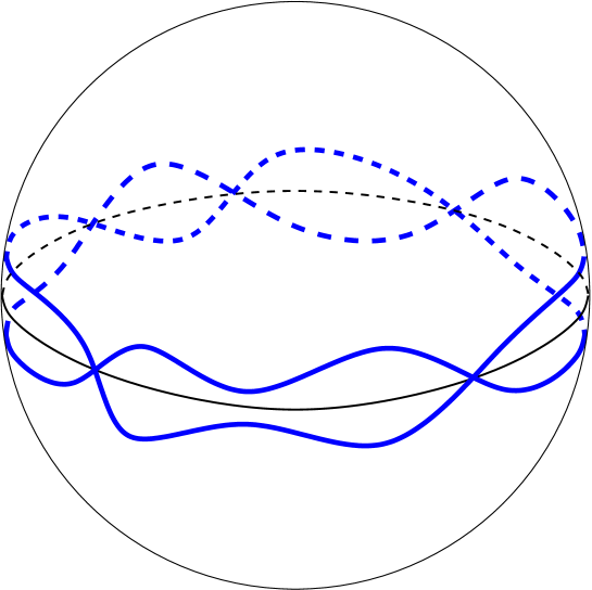
Figure 1. The $g=2$ case

Finally we blow up the $2g+1$ real singular points of $C_{t}$ to get a rational surface $S_{g}$. The birational transform of $C_{t}$ gives a rational curve $C_{g}\subset S_{g}$ which is smooth at its real points.

The $2g+1$ regions of ${\mathbb{S}}^{2}\setminus C_{t}({\mathbb{R}})$ near the equator become a Möbius band on $S_{g}({\mathbb{R}})\setminus C_{g}({\mathbb{R}})$ and the northern and southern hemispheres become $\#g{\mathbb{T}}^{2}$ (with one puncture). Thus

$$\bigl{(}S_{g}({\mathbb{R}}),C_{g}({\mathbb{R}})\bigr{)}\sim{\mathbb{R}}{\mathbb{P}}^{2}\#({\mathbb{S}}^{2},{\mathbb{L}})\#g{\mathbb{T}}^{2}.$$

Proposition 23.

Let $C\subset{\mathbb{P}}^{1}\times{\mathbb{P}}^{1}$ be a real-smooth rational curve defined over ${\mathbb{R}}$. Then $[C({\mathbb{R}})]\in H_{1}({\mathbb{T}}^{2},{\mathbb{Z}}/2)$ is nonzero.

Proof. Let $E_{1},E_{2}$ denote a horizontal (resp. vertical) complex line on ${\mathbb{P}}^{1}\times{\mathbb{P}}^{1}$. Every complex algebraic curve $C$ has homology class $a_{1}E_{1}+a_{2}E_{2}$ for some $a_{1},a_{2}\geq 0$. Furthermore, if $C$ is defined over ${\mathbb{R}}$ then

$$a_{i}=(C\cdot E_{3-i})\equiv\bigl{(}C({\mathbb{R}})\cdot E_{3-i}({\mathbb{R}})\bigr{)}\mod 2.$$

Thus if $[C({\mathbb{R}})]\in H_{1}({\mathbb{T}}^{2},{\mathbb{Z}}/2)$ is zero then $a_{1},a_{2}$ are even. By the adjunction formula

$$2p_{a}(C)-2=\bigl{(}a_{1}E_{1}+a_{2}E_{2}\bigr{)}\cdot\bigl{(}(a_{1}-2)E_{1}+(a_{2}-2)E_{2}\bigr{)}=a_{1}(a_{2}-2)+a_{2}(a_{1}-2),$$

hence $p_{a}(C)=(a_{1}-1)(a_{2}-1)$. Thus, if the $a_{i}$ are even then $p_{a}(C)$ is odd. Therefore, if $C$ is rational then it has an odd number of singular points and at least one of them has to be real.∎

5. Related approximation problems

24Approximation of curves on algebraic surfaces.

When $S$ is a non-rational surface, we can ask for several possible analogs of Theorem 3.

On many surfaces there are no rational curves at all, thus the best one can hope for is approximation by higher genus curves. Even for this, there are several well known obstructions.

First of all, given a real algebraic surface $X$, a necessary condition for a smooth curve $C$ to admit an approximation by an algebraic curve is that its fundamental class $[C]$ belong to the group of algebraic cycles $\operatorname{H}^{1}_{\mathrm{alg}}(X,{\mathbb{Z}}/2)$. The latter group is generally a proper subgroup of the cohomology group $\operatorname{H}^{1}(X,{\mathbb{Z}}/2)$. See [BH61] and [BCR98, Sec.12.4] for details.

The structure of these groups for various real algebraic surfaces of special type is computed in [Man94, Man97, MvH98, Man00, Man03]. These papers contain the classification of totally algebraic surfaces, that is surfaces such that $\operatorname{H}^{1}_{\mathrm{alg}}(S,{\mathbb{Z}}/2)=\operatorname{H}^{1}(S,{\mathbb{Z}}/2)$, among K3, Enriques, bi-elliptic, and properly elliptic surfaces. In particular, if $S$ is a non-orientable surface underlying an Enriques surface or a bi-elliptic surface, then there are simple, connected, closed curves on $S$ with no approximation by any algebraic curve, see [MvH98, Thm.1.1] and [Man03, Thm.0.1].

If $S$ is orientable, there can be further obstructions involving $\operatorname{H}^{1}(S,{\mathbb{Z}})$. For instance, let $S\subset{\mathbb{R}}{\mathbb{P}}^{3}$ be a very general K3 surface. By the Noether–Lefschetz theorem, the Picard group of $S({\mathbb{C}})$ is generated by the hyperplane class. If $S$ is contained in ${\mathbb{R}}^{3}$ then the restriction of ${\mathcal{O}}_{{\mathbb{P}}^{3}}(1)$ to $S$ is trivial, thus only null-homotopic curves can be approximated by algebraic curves.

Note also that if $S$ is a real K3 surface, then by [Man97], there is a totally algebraic real K3 surface real deformation equivalent to $S$ (at least if $S$ is a non-maximal surface) thus in general there is no purely topological obstruction to approximability for real K3 surfaces.

25Approximation of curves on geometrically rational surfaces.

Geometrically rational surface contain many rational curves, so approximation by real-smooth rational curves could be possible. Any geometrically rational surface is totally algebraic but there are not enough automorphisms to approximate all diffeomorphisms, at least if the number of connected components is greater than 2; see [BM11].

Another obstruction arises from the genus formula. For example, let $S$ be a degree $2$ Del Pezzo surface with Picard number $\rho(S)=1$ and $C\subset S$ a curve on it. Then $C\sim-aK_{S}$ for some positive integer $a$ and so $C(C+K_{S})=2a(a-1)$ is divisible by $4$. Thus the arithmetic genus $p_{a}(C)$ is odd hence every real rational curve on $S$ has an odd number of singular points on $S({\mathbb{C}})$. These can not all be complex conjugate, thus every rational curve on $S$ has a real singular point.

It seems, however, that this type of parity obstruction for approximation does not occur on any other geometrically rational surface. We hazard the hope that if $S$ is a geometrically rational surface then every simple, connected, closed curve can be approximated by real-smooth rational curves, save when either $S\sim{\mathbb{T}}^{2}$ or $S$ is isomorphic to a degree $2$ Del Pezzo surface with Picard number $1$.

As another generalization, one can study such problems for singular rational surfaces as in [HM10]. See also the series [CM08], [CM09] for the classification of geometrically rational surfaces with Du Val singularities.

26Approximation of curves on higher dimensional varieties.

As for surfaces, we can hope to approximate every simple, connected, closed curve on a real variety $X$ by a nonsingular rational curve over ${\mathbb{R}}$ only if there are many rational curves on the corresponding complex variety $X({\mathbb{C}})$. First one should consider rational varieties.

Proposition 26.1. Let $X$ be a smooth, projective, real variety of dimension $\geq 3$ that is rational. Then every simple, connected, closed curve $L\subset X({\mathbb{R}})$ can be approximated by smooth rational curves.

Proof. Represent $L$ as the image of an embedding ${\mathbb{S}}^{1}\to X({\mathbb{R}})$. The proof of [BK99] automatically produces approximations by maps $g:{\mathbb{P}}^{1}\to X$ such that $g^{*}T_{X}$ is ample. By an easy lemma (cf. [Kol96, II.3.14]) a general small perturbation of any morphism $g:{\mathbb{P}}^{1}\to X$ such that $g^{*}T_{X}$ is ample is an embedding. ∎

The next class to consider is geometrically rational varieties, or, more generally, rationally connected varieties [Kol96, Chap.IV].

Let $X$ be a smooth, real variety such that $X({\mathbb{C}})$ is rationally connected. By a combination of [Kol99, Cor.1.7] and [Kol04, Thm.23], if $p_{1},\dots,p_{s}\in X({\mathbb{R}})$ are in the same connected component then there is a rational curve $g:{\mathbb{P}}^{1}\to X$ passing through all of them. By the previous argument, we can even choose $g$ to be an embedding if $\dim X\geq 3$. Thus $X$ contains plenty of smooth rational curves.

Nonetheless, we believe that usually not every homotopy class of $X({\mathbb{R}})$ can be represented by rational curves. The following example illustrates some of the possible obstructions.

Example 26.2. Let $q_{1},q_{2},q_{3}$ be quadrics such that $C:=(q_{1}=q_{2}=q_{3}=0)\subset{\mathbb{P}}^{4}$ is a smooth curve with $C({\mathbb{R}})\neq\emptyset$. Consider the family of 3–folds

$$X_{t}:=\bigl{(}q_{1}^{2}+q_{2}^{2}+q_{3}^{2}-t\bigl{(}x_{0}^{4}+\cdots+x_{4}^{4})=0\bigr{)}\subset{\mathbb{P}}^{4}$$

For $0<t\ll 1$, the real points $X_{t}({\mathbb{R}})$ form an ${\mathbb{S}}^{2}$-bundle over $C({\mathbb{R}})$. We conjecture that if $0<t\ll 1$, then every rational curve $g\colon{\mathbb{P}}^{1}\to X_{t}$ gives a null-homotopic map $g\colon{\mathbb{R}}{\mathbb{P}}^{1}\to X_{t}({\mathbb{R}})$.

We do not know how to prove this, but the following argument shows that if $g_{t}:{\mathbb{P}}^{1}\to X_{t}$ is a continuous family of rational curves defined for every $0<t\ll 1$, then $g_{t}:{\mathbb{R}}{\mathbb{P}}^{1}\to X_{t}({\mathbb{R}})$ is null-homotopic. More precisely, the images $g_{t}({\mathbb{R}}{\mathbb{P}}^{1})\subset X_{t}({\mathbb{R}})$ shrink to a point as $t\to 0$.

Indeed, otherwise by taking the limit as $t\to 0$, we get a non-constant map $\tilde{g}_{0}:{\mathbb{P}}^{1}\to C$. However, the genus of $C$ is 5, hence every map ${\mathbb{P}}^{1}\to C$ is constant. (A priori, the limit, taken in the moduli space of stable maps as in [FP97], is a morphism $g_{0}:B\to X_{0}$ where $B$ is a (usually reducible) real curve with only nodes as singularities such that $h^{1}(B,{\mathcal{O}}_{B})=0$. For such curves, the set of real points $B({\mathbb{R}})$ is a connected set. Thus the image of $B({\mathbb{R}})$ is a connected subset of $X_{0}({\mathbb{R}})$ that contains at least 2 distinct points. Since $X_{0}({\mathbb{R}})=C({\mathbb{R}})$, one of the irreducible components of $B$ gives a non-constant map $\tilde{g}_{0}:{\mathbb{P}}^{1}\to C$.)

Unfortunately, this only implies that if we have a sequence $t_{i}\to 0$ and a sequence of homotopically nontrivial rational curves $g_{t_{i}}:{\mathbb{P}}^{1}\to X$ then their degree must go to infinity. We did not exclude the possibility that, as $t_{i}\to 0$, we have higher and higher degree maps approximating non null-homotopic loops.

We do not have a conjecture about which homotopy classes give obstructions. On the other hand, while we do not have much evidence, the following could be true.

Conjecture 26.3. Let $X$ be a smooth, rationally connected variety defined over ${\mathbb{R}}$. Then a $C^{\infty}$ map ${\mathbb{S}}^{1}\to X({\mathbb{R}})$ can be approximated by rational curves iff it is homotopic to a rational curve ${\mathbb{R}}{\mathbb{P}}^{1}\to X({\mathbb{R}})$.

References

- [AK03] Carolina Araujo and János Kollár, Rational curves on varieties, Higher dimensional varieties and rational points (Budapest, 2001), Bolyai Soc. Math. Stud., vol. 12, Springer, Berlin, 2003, pp. 13–68. MR 2011743 (2004k:14049)
- [BCR98] Jacek Bochnak, Michel Coste, and Marie-Françoise Roy, Real algebraic geometry, Ergebnisse der Mathematik und ihrer Grenzgebiete (3), vol. 36, Springer-Verlag, Berlin, 1998, Translated from the 1987 French original, Revised by the authors. MR 1659509 (2000a:14067)
- [BH61] Armand Borel and André Haefliger, La classe d’homologie fondamentale d’un espace analytique, Bull. Soc. Math. France 89 (1961), 461–513. MR 0149503 (26 #6990)
- [BH07] Indranil Biswas and Johannes Huisman, Rational real algebraic models of topological surfaces, Doc. Math. 12 (2007), 549–567. MR 2377243 (2008m:14115)
- [BK99] J. Bochnak and W. Kucharz, The Weierstrass approximation theorem for maps between real algebraic varieties, Math. Ann. 314 (1999), no. 4, 601–612. MR 1709103 (2001c:14082)
- [BM11] Jérémy Blanc and Frédéric Mangolte, Geometrically rational real conic bundles and very transitive actions, Compos. Math. 147 (2011), no. 1, 161–187. MR 2771129 (2012b:14116)
- [CM08] Fabrizio Catanese and Frédéric Mangolte, Real singular del Pezzo surfaces and 3-folds fibred by rational curves. I, Michigan Math. J. 56 (2008), no. 2, 357–373. MR 2492399 (2010f:14063)
- [CM09] by same author, Real singular del Pezzo surfaces and 3-folds fibred by rational curves. II, Ann. Sci. Éc. Norm. Supér. (4) 42 (2009), no. 4, 531–557. MR 2568875 (2011c:14109)
- [Com14] Annibale Comessatti, Sulla connessione delle superficie razionali reali, Ann. Mat. Pura Appl. 23 (1914), 215–283.
- [DZ01] Igor V. Dolgachev and De-Qi Zhang, Coble Rational Surfaces, Amer. Jour. Math. 123 (2001), 79–114,
- [FP97] W. Fulton and R. Pandharipande, Notes on stable maps and quantum cohomology, Algebraic geometry—Santa Cruz 1995, Proc. Sympos. Pure Math., vol. 62, Amer. Math. Soc., Providence, RI, 1997, pp. 45–96. MR MR1492534 (98m:14025)
- [HK11a] DongSeon Hwang and JongHae Keum, Algebraic Montgomery-Yang problem: the non-cyclic case, Math. Ann. 350 (2011), no. 3, 721–754. MR 2805643 (2012k:14047)
- [HK11b] by same author, The maximum number of singular points on rational homology projective planes, J. Algebraic Geom. 20 (2011), no. 3, 495–523. MR 2786664 (2012c:14078)
- [HK12] by same author, Construction of singular rational surfaces of Picard number one with ample canonical divisor, Proc. Amer. Math. Soc. 140 (2012), no. 6, 1865–1879. MR 2888175
- [HM09] Johannes Huisman and Frédéric Mangolte, The group of automorphisms of a real rational surface is -transitive, Bull. Lond. Math. Soc. 41 (2009), no. 3, 563–568. MR 2506841 (2010m:14042)
- [HM10] by same author, Automorphisms of real rational surfaces and weighted blow-up singularities, Manuscripta Math. 132 (2010), no. 1-2, 1–17. MR 2609286 (2011j:14123)
- [Keu11] JongHae Keum, A fake projective plane constructed from an elliptic surface with multiplicities , Sci. China Math. 54 (2011), no. 8, 1665–1678. MR 2824965 (2012h:14100)
- [KM98] János Kollár and Shigefumi Mori, Birational geometry of algebraic varieties, Cambridge Tracts in Mathematics, vol. 134, Cambridge University Press, Cambridge, 1998, With the collaboration of C. H. Clemens and A. Corti, Translated from the 1998 Japanese original. MR 1658959 (2000b:14018)
- [KM09] János Kollár and Frédéric Mangolte, Cremona transformations and diffeomorphisms of surfaces, Adv. Math. 222 (2009), no. 1, 44–61. MR 2531367 (2010g:14016)
- [Kol96] János Kollár, Rational curves on algebraic varieties, Ergebnisse der Mathematik und ihrer Grenzgebiete. 3. Folge., vol. 32, Springer-Verlag, Berlin, 1996. MR 1440180 (98c:14001)
- [Kol99] by same author, Rationally connected varieties over local fields, Ann. of Math. (2) 150 (1999), no. 1, 357–367. MR MR1715330 (2000h:14019)
- [Kol00] by same author, Real algebraic threefolds. IV. Del Pezzo fibrations, Complex analysis and algebraic geometry, de Gruyter, Berlin, 2000, pp. 317–346. MR MR1760882 (2001c:14087)
- [Kol01] by same author, The topology of real algebraic varieties, Current developments in mathematics, 2000, Int. Press, Somerville, MA, 2001, pp. 197–231. MR MR1882536 (2002m:14046)
- [Kol04] by same author, Specialization of zero cycles, Publ. Res. Inst. Math. Sci. 40 (2004), no. 3, 689–708. MR MR2074697
- [Kol08] by same author, Is there a topological Bogomolov-Miyaoka-Yau inequality?, Pure Appl. Math. Q. 4 (2008), no. 2, part 1, 203–236. MR 2400877 (2009b:14086)
- [KSC04] János Kollár, Karen E. Smith, and Alessio Corti, Rational and nearly rational varieties, Cambridge Studies in Advanced Mathematics, vol. 92, Cambridge University Press, Cambridge, 2004. MR 2062787 (2005i:14063)
- [Man66] Ju. I. Manin, Rational surfaces over perfect fields, Inst. Hautes Études Sci. Publ. Math. (1966), no. 30, 55–113. MR 0225780 (37 #1373)
- [Man94] Frédéric Mangolte, Une surface réelle de degré dont l’homologie est entièrement engendrée par des cycles algébriques, C. R. Acad. Sci. Paris Sér. I Math. 318 (1994), no. 4, 343–346. MR 1267612 (95g:14060)
- [Man97] by same author, Cycles algébriques sur les surfaces réelles, Math. Z. 225 (1997), no. 4, 559–576. MR 1466402 (98f:14046)
- [Man00] by same author, Surfaces elliptiques réelles et inégalité de Ragsdale-Viro, Math. Z. 235 (2000), no. 2, 213–226. MR 1795505 (2002b:14071)
- [Man03] by same author, Cycles algébriques et topologie des surfaces bielliptiques réelles, Comment. Math. Helv. 78 (2003), no. 2, 385–393. MR 1988202 (2005b:14020)
- [MvH98] Frédéric Mangolte and Joost van Hamel, Algebraic cycles and topology of real Enriques surfaces, Compositio Math. 110 (1998), no. 2, 215–237. MR 1602080 (99k:14015)
- [Seg51] Beniamino Segre, On the rational solutions of homogeneous cubic equations in four variables, Math. Notae 11 (1951), 1–68. MR 0046064 (13,678d)
- [Sha74] Igor R. Shafarevich, Basic algebraic geometry, Springer-Verlag, New York, 1974, Die Grundlehren der mathematischen Wissenschaften, Band 213. MR 0366917 (51 #3163)