Robust Independent Component Analysis
via Minimum Divergence Estimation

Abstract

Independent component analysis (ICA) has been shown to be useful in many applications. However, most ICA methods are sensitive to data contamination and outliers. In this article we introduce a general minimum $U$-divergence framework for ICA, which covers some standard ICA methods as special cases. Within the $U$-family we further focus on the $\gamma$-divergence due to its desirable property of super robustness, which gives the proposed method $\gamma$-ICA. Statistical properties and technical conditions for the consistency of $\gamma$-ICA are rigorously studied. In the limiting case, it leads to a necessary and sufficient condition for the consistency of MLE-ICA. This necessary and sufficient condition is weaker than the condition known in the literature. Since the parameter of interest in ICA is an orthogonal matrix, a geometrical algorithm based on gradient flows on special orthogonal group is introduced to implement $\gamma$-ICA. Furthermore, a data-driven selection for the $\gamma$ value, which is critical to the achievement of $\gamma$-ICA, is developed. The performance, especially the robustness, of $\gamma$-ICA in comparison with standard ICA methods is demonstrated through experimental studies using simulated data and image data.

Key words and phrases: $\beta$-divergence; $\gamma$-divergence; geodesic; independent component analysis; minimum divergence; robust statistics; special orthogonal group.

1 Introduction

Consider the following generative model for independent component analysis (ICA)

$$X=AS+\mu,$$ (1)

where the elements of the non-Gaussian source vector $S\in\mathbb{R}^{p}$ are mutually independent with zero mean, $A\in\mathbb{R}^{p\times p}$ is an unknown nonsingular mixing matrix, $X\in\mathbb{R}^{p}$ is an observable random vector (signal), and $\mu=E(X)\in\mathbb{R}^{p}$ is a shift parameter. Let $Z=\Sigma^{-1/2}(X-\mu)$ be the whitened data of $X$, where $\Sigma={\rm cov}(X)$. An equivalent expression of model (1) in $Z$-scale is

$$Z=\widetilde{A}S,$$ (2)

where $\widetilde{A}=\Sigma^{-1/2}A$ is the mixing matrix in $Z$-scale. It is reported in literature that prewhitening the data can make the ICA inference procedure more stable. In the rest of the discussion, we will work with model (2) in estimating the mixing matrix $\widetilde{A}$ based on the prewhitened $Z$. It is easy to transform back to the original $X$-scale via $A=\Sigma^{1/2}\widetilde{A}$. Note that both $\widetilde{A}$ and $S$ are unknown, and there exists the identifiability problem. This can be seen from the fact that $Z=\widetilde{A}S=(\widetilde{A}M)(M^{-1}S)$ for any nonsingular diagonal matrix $M$. To make $\widetilde{A}$ identifiable, we assume the following conventional conditions for $S$:

$$E(S)=0\quad{\rm and}\quad{\rm cov}(S)=I_{p},$$ (3)

where $I_{p}\in\mathbb{R}^{p\times p}$ is the identity matrix. It then implies that $\Sigma=AA^{\top}$ and

$$I_{p}={\rm cov}(Z)=\widetilde{A}\,{\rm cov}(S)\,\widetilde{A}^{\top}=\widetilde{A}\widetilde{A}^{\top},$$ (4)

which means that the mixing matrix $\widetilde{A}$ in $Z$-scale is orthogonal. We will use notation ${\cal O}_{p}$ to denote the space of orthogonal matrices in $\mathbb{R}^{p\times p}$. Note that, if $\widetilde{A}\in{\cal O}_{p}$ is a parameter of model (2), so is $-\widetilde{A}\in{\cal O}_{p}$. Thus, to fix one direction, we consider $\widetilde{A}\in{\cal SO}_{p}$, where ${\cal SO}_{p}\subset{\cal O}_{p}$ consists of orthogonal matrices with determinant one. This set ${\cal SO}_{p}$ is called the special orthogonal group. The main purpose of ICA is to estimate the orthogonal $\widetilde{A}\in{\cal SO}_{p}$ based on the whitened data $\{z_{i}\}_{i=1}^{n}$, or equivalently, to look for a recovering matrix $W\in{\cal SO}_{p}$ so that components in $Y=:W^{\top}Z=(w_{1}^{\top}Z,\ldots,w_{p}^{\top}Z)^{\top}$ have the maximum degree of independence. In the latter case, $W$ provides an estimate of $\widetilde{A}$.

We first briefly review some existing methods for ICA. One idea is to estimate $W$ via minimizing the mutual information. Let $g_{Y}$ be the joint probability density function of $Y=(Y_{1},\dots,Y_{p})^{\top}$, and $g_{Y_{j}}$ be the marginal probability density function of $Y_{j}$. The mutual information, denoted by $I(Y_{1},\dots,Y_{p})$, among random variables $(Y_{1},\ldots,Y_{p})$, is defined to be

$$I(Y_{1},\ldots,Y_{p}):=\sum_{j=1}^{p}H(Y_{j})-H(Y),$$ (5)

where $H(Y)=-\int g_{Y}\ln g_{Y}$ and $H(Y_{j})=-\int g_{Y_{j}}\ln g_{Y_{j}}$ are the Shannon entropy. Ideally, if $W$ is properly chosen so that $Y$ has independent components, then $g_{Y}=\prod_{j}g_{Y_{j}}$ and, hence, $I(Y_{1},\ldots,Y_{p})=0$. Thus, via minimizing $I(Y_{1},\ldots,Y_{p})$ with respect to $W$, it leads to an estimate of $W$. Another method is to estimate $W$ via maximizing the negentropy, which is equivalent to minimizing mutual information as described below. The negentropy of $Y$ is defined to be

$$J(Y)=H(Y^{\prime})-H(Y),$$ (6)

where $Y^{\prime}$ is a Gaussian random vector having the same covariance matrix as $Y$ (Hyvärinen and Oja, 2000). It can be deduced that

$$I(Y_{1},\ldots,Y_{p})=J(Y)-\sum_{j=1}^{p}J(Y_{j})-H(Y^{\prime})+\sum_{j=1}^{p}H(Y_{j}^{\prime})=J(Y)-\sum_{j=1}^{p}J(Y_{j}),$$ (7)

where the second equality holds since, by ${\rm cov}(Y^{\prime})={\rm cov}(Y)=I_{p}$, $H(Y^{\prime})=\sum_{j=1}^{p}H(Y_{j}^{\prime})$. Moreover, as $Y=W^{\top}Z$ with $W\in{\cal SO}_{p}$, we have $J(Y)=J(Z)$, which does not depend on $W$. That is, the negentropy is invariant under orthogonal transformation. Thus, minimizing the mutual information $I(Y_{1},\ldots,Y_{p})$ is equivalent to maximizing the negentropy $\sum_{j=1}^{p}J(Y_{j})$. The negentropy $J(Y_{j})$, however, involves the unknown density $g_{Y_{j}}$. To avoid nonparametric estimation of $g_{Y_{j}}$, one can use the following approximation (Hyvärinen, 1998) via a non-quadratic contrast function $G(\cdot)$,

$$J(Y_{j})\approx J_{G}(Y_{j})=[E\{G(Y_{j})\}-E\{G(\nu)\}]^{2},$$ (8)

where $\nu$ is a random variable having the standard normal distribution. Here $J_{G}$ can be treated as a measure of non-Gaussianity, and minimizing the sample analogue of $J_{G}(Y_{j})$ to search $W$ corresponds to the fast-ICA (Hyvärinen, 1999).

Another widely used estimation criterion for $W$ is via maximizing the likelihood. Under model (2) and by modeling $g_{Y_{j}}=f_{j}$ with some known probability density function $f_{j}$, the density function of $Z$ takes the form

$$f_{Z}(z;W) = |{\rm det}(W)|\,\prod_{j=1}^{p}f_{j}(w_{j}^{\top}z)=\prod_{j=1}^{p}f_{j}(w_{j}^{\top}z)$$ (9)

since $W\in{\cal SO}_{p}$ and hence ${\rm det}(W)=1$. The MLE-ICA then searches the optimum $W$ via

$$\mathop{\rm argmin}_{W\in{\cal SO}_{p}}\mathcal{D}_{0}\left({\widehat{g}_{n}},f_{Z}(\cdot\,;W)\right),$$ (10)

where $\mathcal{D}_{0}(g,f)=-\int g\ln(f/g)$ is the Kullback-Leibler divergence (KL-divergence), and ${\widehat{g}_{n}}$ is the empirical distribution of $\{z_{i}\}_{i=1}^{n}$. Possible choices of $f_{j}$ include $f_{j}(s)=c_{1}\exp(-c_{2}s^{4})$ for sub-Gaussian models, and $f_{j}(s)=c_{1}/{\rm cosh}(c_{2}s)$ for super-Gaussian models, where $c_{1}$ and $c_{2}$ are constants so that $f_{j}$ is a probability density function. It can be seen from (9) that, for any row permutation matrix $\Pi$, we have $f_{Z}(z;\Pi\,W)=f_{Z}(z;W)$. That is, we can estimate and identify $\widetilde{A}$ only up to its row-permutation.

As will become clear later that the above mentioned methods are all related to minimizing the KL-divergence, which is not robust in the presence of outliers. Outliers, however, frequently appear in real data analysis, and a robust ICA inference procedure becomes necessary. For the purpose of robustness, instead of the KL-divergence, Mihoko and Eguchi (2002) considers the minimum $\beta$-divergence estimation for $W$ ($\beta$-ICA). The issues of consistency and robustness of $\beta$-ICA are discussed therein. On the other hand, the $\gamma$-divergence, which can be induced from $\beta$-divergence, is shown to be super robust (Fujisawa and Eguchi, 2008) against data contamination. It is our aim in this paper to propose a unified ICA inference procedure by minimum divergence estimation. Moreover, due to the property of super robustness, we will focus on the case of $\gamma$-divergence and propose a robust ICA procedure, called $\gamma$-ICA. Hyvärinen, Karhnen and Oja (2001) have provided a sufficient condition to ensure the validity of MLE-ICA under the orthogonality constraint of $W$, in the sense of being able to recover all independent components. Amari, Chen, and Cichocki (1997) studied necessary and sufficient conditions for consistency under a different constraint of $W$, and this consistency result is further extended by Mihoko and Eguchi (2002) to the case of $\beta$-ICA. In this work, we also derive necessary and sufficient conditions for the consistency of $\gamma$-ICA. In the limiting case $\gamma\to 0$, our necessary and sufficient condition for the consistency of MLE-ICA is weaker than the condition stated in Hyvärinen, Karhnen and Oja (2001). To the best of our knowledge, this result is not explored in existing literature.

Some notation is defined here for the convenience of reference. For any $M\in\mathbb{R}^{p\times p}$, let $K_{p}\in\mathbb{R}^{p^{2}\times p^{2}}$ be the commutation matrix such that ${\rm vec}(M^{\top})=K_{p}{\rm vec}(M)$; $M>0$ (resp. $<0$) means $M$ is strictly positive (resp. negative) definite; and $\exp(M):=\sum_{k=0}^{\infty}\frac{M^{k}}{k!}$ is the matrix exponential. Note that ${\rm det}(\exp(M))=\exp({\rm tr}(M))$ for any nonsingular square matrix $M$. For a lower triangular matrix $M$ with 0 diagonals, ${\rm vecp}(M)$ stacks the nonzero elements of the columns of $M$ into a vector with length $p(p-1)/2$. There exist matrices $P\in\mathbb{R}^{p(p-1)/2\times p^{2}}$ and $Q\in\mathbb{R}^{p^{2}\times p(p-1)/2}$ such that ${\rm vecp}(M)=P{\rm vec}(M)$ and ${\rm vec}(M)=Q{\rm vecp}(M)$. Each column vector of $Q$ is of the form $(e_{i}\otimes e_{j})$, $i<j$, where $e_{i}\in\mathbb{R}^{p}$ is a vector with a one in the $i$-th position and 0 elsewhere, and $\otimes$ is the Kronecker product. $I_{p}\in\mathbb{R}^{p\times p}$ is the identity matrix and $1_{p}\in\mathbb{R}^{p}$ is the $p$-vector of ones.

The rest of this paper is organized as follows. A unified framework for ICA estimation by minimum divergence is introduced in Section 2. A robust $\gamma$-ICA procedure is developed in Section 3, wherein the related statistical properties are studied. A geometrical implementation algorithm for $\gamma$-ICA is further illustrated in Section 4. In Section 5, the issue of selecting $\gamma$ value is discussed. Numerical studies are conducted in Section 6 to demonstrate the robustness of $\gamma$-ICA. The paper is ended with a conclusion in Section 7. All the proofs are placed in Appendix.

2 Minimum ${\bm{U}}$-divergence estimation for ICA

In this section we introduce a general framework for ICA by means of a minimum $U$-divergence, which covers the existing methods reviewed in Section 1. The aim of ICA is to search a matrix $W\in{\cal SO}_{p}$ so that the joint probability density function $g_{Y}$ for $Y=W^{\top}Z$ is as close to marginal product $\prod_{j}g_{Y_{j}}$ as possible. This aim then motivates estimating $W$ by minimizing a distance metric between $g_{Y}$ and $\prod_{j}g_{Y_{j}}$. A general estimation scheme for $W$ can be formulated through the following minimization problem

$$\min_{W\in{\cal SO}_{p}}\mathcal{D}(g_{Y},\prod_{j}g_{Y_{j}}),$$ (11)

where $\mathcal{D}(\cdot,\cdot)$ is a divergence function. Different choices of $\mathcal{D}$ will lead to different estimation criteria for ICA. Here we will consider a general class of divergence functions, the $U$-divergence (Murata et al., 2004; Eguchi, 2009), as described below.

The $U$-divergence is a very general class of divergence functions. Consider a strictly convex function $U(t)$ defined on $\mathbb{R}$, or on some interval of $\mathbb{R}$ where $U(t)$ is well-defined. Let $\xi=\dot{U}^{-1}$ be the inverse function of $\dot{U}:=\frac{d}{dt}U(t)$. Consider

$$\mathcal{D}_{U}(g,f) = \int U(\xi(f))-U(\xi(g))-\dot{U}(\xi(g))\cdot\{\xi(f)-\xi(g)\}$$ (12)

$$= \int U(\xi(f))-U(\xi(g))-g\cdot\{\xi(f)-\xi(g)\},$$

which defines a mapping from ${\cal M}_{U}\times{\cal M}_{U}$ to $[0,\infty)$, where ${\cal M}_{U}=\left\{f:\int U(\xi(f))<\infty,\;f\geq 0\right\}$. Define the $U$-cross entropy by

$$C_{U}(g,f)=-\int\xi(f)g+\int U(\xi(f)),$$ (13)

and the $U$-entropy by $H_{U}(g)=C_{U}(g,g)$. Then the $U$-divergence can be written as

$$\mathcal{D}_{U}(g,f)=C_{U}(g,f)-H_{U}(g)\geq 0.$$ (14)

In the subsequent subsections, we will introduce some special cases of $U$-divergence, which will lead to specific methods of ICA.

2.1 KL-divergence

By taking the $(U,\xi)$ pair

$$U(t)=\exp(t),\quad\xi(t)=\ln t,$$ (15)

the corresponding $U$-divergence is equivalent to the KL-divergence $D_{0}$. In this case, it can be deduced that

$$\mathcal{D}_{0}(g_{Y},\prod_{j}g_{Y_{j}})=I(Y_{1},\ldots,Y_{p}),$$ (16)

where $I(Y_{1},\ldots,Y_{p})$ is the mutual information defined in (5). As described in Section 1 that

$$\mathop{\rm argmin}_{W\in{\cal SO}_{p}}I(Y_{1},\ldots,Y_{p})=\mathop{\rm argmax}_{W\in{\cal SO}_{p}}\sum_{j=1}^{p}J(Y_{j})\approx\mathop{\rm argmax}_{W\in{\cal SO}_{p}}\sum_{j=1}^{p}J_{G}(Y_{j}),$$ (17)

we conclude that the following criteria, minimum mutual information, maximum negentropy, and fast-ICA, are all special cases of (11). On the other hand, observe that

$$\mathcal{D}_{0}(g_{Y}(y),\prod_{j}g_{Y_{j}}(y_{j}))=\mathcal{D}_{0}(g_{Z}(z),\prod_{j}g_{Y_{j}}(w_{j}^{\top}z)),$$ (18)

where $g_{Z}$ is the joint probability density function of $Z$. If we consider the model $g_{Y_{j}}=f_{j}$, and if we estimate $g_{Z}$ by its empirical probability mass function ${\widehat{g}_{n}}$, minimizing (18) is equivalent to MLE-ICA in (10). In summary, choosing the KL-divergence $D_{0}$ covers minimum mutual information, maximum negentropy, fast-ICA, and MLE-ICA.

2.2 $\bm{\beta}$-divergence

Consider the convex set ${\cal M}_{\beta+1}:=\left\{f:\int f^{\beta+1}<\infty,~{}f\geq 0\right\}$. Take the $(U,\xi)$ pair

$$U(t)=\frac{1}{1+\beta}(1+\beta t)^{\frac{\beta+1}{\beta}},\quad\xi(t)=\frac{1}{\beta}(t^{\beta}-1).$$ (19)

The resulting $U$-divergence defined on ${\cal M}_{\beta+1}\times{\cal M}_{\beta+1}$ is calculated to be

$$\mathcal{B}_{\beta}(g,f)=\frac{1}{\beta}\int(g^{\beta}-f^{\beta})g-\frac{1}{\beta+1}\int(g^{\beta+1}-f^{\beta+1})\$$ (20)

which is called $\beta$-divergence (Mihoko and Eguchi, 2002), or density power divergence (Basu et al., 1998). Note that $\mathcal{B}_{\beta}(g,f)=0$ if and only if $f=\lambda g$ for some $\lambda>0$. In the limiting case $\lim_{\beta\to 0}\mathcal{B}_{\beta}=\mathcal{D}_{0}$, it gives the KL-divergence. If we replace $\mathcal{D}_{0}$ in (10) by $\mathcal{B}_{\beta}$, it gives the $\beta$-ICA of Mihoko and Eguchi (2002).

2.3 $\bm{\gamma}$-divergence

The $\gamma$-divergence can be obtained from $\beta$-divergence through a $U$-volume normalization,

$$\mathcal{D}_{\gamma}(g,f):=\mathcal{B}_{\gamma}\left(\alpha(g)\cdot g,\alpha(f)\cdot f\right),$$

where $\mathcal{B}_{\gamma}$ is defined the same way as (20) with the plug-in $\beta=\gamma$, and where $\alpha(f)$ is some normalizing constant. Here we adopt the following normalization, called the volume-mass-one normalization,

$$\int U\big{(}\xi(\alpha(f)\cdot f(x))\big{)}dx=1.$$ (21)

It leads to $\alpha(f)=(\gamma+1)^{1/(\gamma+1)}\|f\|_{\gamma+1}^{-1}$. Then,

$$\mathcal{D}_{\gamma}(g,f)=\frac{\gamma+1}{\gamma}\left\{1-\int\left(\frac{f(x)}{\|f\|_{\gamma+1}}\right)^{\gamma}\frac{g(x)}{\|g\|_{\gamma+1}}dx\right\}.$$ (22)

It can be seen that $\gamma$-divergence is scale invariant. Moreover, $\mathcal{D}_{\gamma}(g,f)=0$ if and only if $f=\lambda g$ for some $\lambda>0$. The $\gamma$-divergence, indexed by a power parameter $\gamma$, is a generalization of KL-divergence. In the limiting case $\lim_{\gamma\to 0}\mathcal{D}_{\gamma}=\mathcal{D}_{0}$, it gives the KL-divergence. It is well known that MLE (based on minimum KL-divergence) is not robust to outliers. On the other hand, the minimum $\gamma$-divergence estimation is shown to be super robust (Fujisawa and Eguchi, 2008) against data contamination. Hence, we will adopt $\gamma$-divergence to propose our robust $\gamma$-ICA procedure. In particular, the main idea of $\gamma$-ICA is to replace $\mathcal{D}_{0}$ in (10) by $\mathcal{D}_{\gamma}$. Though the idea is straightforward, there are many issues need to be studied. Detailed inference procedure and statistical properties of $\gamma$-ICA are discussed in Section 3.

3 The $\bm{\gamma}$-ICA inference procedure

The ICA is actually a two-stage process. First, we need to whiten the data. The whitened data are then used for the recovery of independent sources. Since the main purpose of this study is to develop a robust ICA inference procedure, the robustness for both data prewhitening and independent source recovery should be guaranteed. Here we will utilize the $\gamma$-divergence to introduce a robust prewhitening method called $\gamma$-prewhitening, followed by illustrating $\gamma$-ICA based on the prewhitened data. In practice, the $\gamma$ value for $\gamma$-divergence should also be determined. In the rest of discussion, we will assume $\gamma$ is given, and leave the discussion of its selection to Section 5.

3.1 $\bm{\gamma}$-prewhitening

Although prewhitening is always possible by a straightforward standardization of $X$, there exists the issue of robustness of such a whitening procedure. It is well known that empirical moment estimates of $(\mu,\Sigma)$ are very sensitive to outliers. In Mollah, Eguchi and Minami (2007), the authors proposed a robust $\beta$-prewhitening procedure. In particular, let $\xi_{\mu,\Sigma}(x)$ be the probability density function of $p$-variate normal distribution with mean $\mu$ and covariance $\Sigma$, and let $\widehat{g}_{X}(x)$ be the empirical distribution based on data $\{x_{i}\}_{i=1}^{n}$. With a given $\beta$, Mollah et al. (2007) proposed the following minimum $\beta$-divergence estimators

$$(\widehat{\kappa},\widehat{\mu},\widehat{\Sigma})=\mathop{\rm argmin}_{\kappa,\mu,\Sigma}\mathcal{B}_{\beta}(\widehat{g}_{X},\kappa\cdot\xi_{\mu,\Sigma}),$$ (23)

and then suggested to use $(\widehat{\mu},\widehat{\Sigma})$ for whitening the data. Interestingly, $(\widehat{\mu},\widehat{\Sigma})$ can also be derived from the minimum $\gamma$-divergence as

$$(\widehat{\mu},\widehat{\Sigma})=\mathop{\rm argmin}_{\mu,\Sigma}\mathcal{D}_{\gamma}(\widehat{g}_{X},\xi_{\mu,\Sigma}).$$ (24)

At the stationarity of (24), the solutions $(\widehat{\mu},\widehat{\Sigma})$ will satisfy

$$\widehat{\mu}=\frac{\sum_{i=1}^{n}d_{i}^{\gamma}(\widehat{\mu},\widehat{\Sigma})\cdot x_{i}}{\sum_{i=1}^{n}d_{i}^{\gamma}(\widehat{\mu},\widehat{\Sigma})}\quad{\rm and}\quad\widehat{\Sigma}=(1+\gamma)\cdot\frac{\sum_{i=1}^{n}d_{i}^{\gamma}(\widehat{\mu},\widehat{\Sigma})\cdot(x_{i}-\widehat{\mu})(x_{i}-\widehat{\mu})^{\top}}{\sum_{i=1}^{n}d_{i}^{\gamma}(\widehat{\mu},\widehat{\Sigma})},$$ (25)

where

$$d_{i}(\mu,\Sigma)=\exp\left\{-\frac{1}{2}(x_{i}-\mu)^{\top}\Sigma^{-1}(x_{i}-\mu)\right\}.$$

The robustness property of $(\widehat{\mu},\widehat{\Sigma})$ can be found in Mollah et al. (2007). We call the prewhitening procedure

$$z_{i}=\widehat{\Sigma}^{-1/2}(x_{i}-\widehat{\mu}),\quad i=1,\ldots,n$$ (26)

the $\gamma$-prewhitening. The whitened data $\{z_{i}\}_{i=1}^{n}$ then enter the $\gamma$-ICA estimation procedure.

3.2 Estimation of $\gamma$-ICA

We are now in the position to develop our $\gamma$-ICA based on the $\gamma$-prewhitened data $\{z_{i}\}_{i=1}^{n}$. As discussed in Section 2.3, the $W$ estimator is derived from

$$\widehat{W}=\mathop{\rm argmin}_{W\in{\cal SO}_{p}}\mathcal{D}_{\gamma}({\widehat{g}_{n}},f_{Z}(\cdot;W))$$ (27)

where $f_{Z}(z;W)=\prod_{j=1}^{p}f_{j}(w_{j}^{\top}z)$ and $f_{j}$ is the working model for $g_{Y_{j}}$. Since $W\in{\cal SO}_{p}$,

$$\int f_{Z}^{\gamma+1}(z;W)dz=|{\rm det}(W)|\prod_{j=1}^{p}\int f_{j}^{\gamma+1}(y_{j})dy_{j}=\prod_{j=1}^{p}\int f_{j}^{\gamma+1}(y_{j})dy_{j},$$

which does not involve $W$. Thus, $\widehat{W}$ can be equivalently obtained via

$$\widehat{W}=\mathop{\rm argmax}_{W\in{\cal SO}_{p}}{\cal L}(W):=\mathop{\rm argmax}_{W\in{\cal SO}_{p}}\,\frac{1}{n}\sum_{i=1}^{n}\left\{\prod_{j=1}^{p}f_{j}^{\gamma}(w_{j}^{\top}z_{i})\right\}.$$ (28)

Finally, the mixing matrix $A$ is estimated by $\widehat{A}=\widehat{\Sigma}^{1/2}\widehat{W}$. Let $f(W^{\top}z)=\prod_{j=1}^{p}f_{j}(w_{j}^{\top}z)$ and

$$\phi(W^{\top}z):=\left[\phi_{1}(w_{1}^{\top}z),\dots,\phi_{p}(w_{p}^{\top}z)\right]^{\top},\;\;{\rm where}\;\;\phi_{j}(y)=\frac{d}{dy}\ln f_{j}(y).$$

We have the following proposition.

Proposition 1.

At the stationarity, the maximizer $\widehat{W}$ defined in (28) will satisfy

$$\frac{1}{n}\sum_{i=1}^{n}f^{\gamma}(\widehat{W}^{\top}z_{i})\left\{\widehat{W}^{\top}z_{i}\,\left[\phi(\widehat{W}^{\top}z_{i})\right]^{\top}-\phi(\widehat{W}^{\top}z_{i})\left[\widehat{W}^{\top}z_{i}\right]^{\top}\right\}=0.$$ (29)

From Proposition 1, it can be easily seen the robustness nature of $\gamma$-ICA: the stationary equation is a weighted sum with the weight function $f^{\gamma}$. When $\gamma>0$, an outlier with extreme value will contribute less to the stationary equation. In the limiting case of $\gamma\to 0$, which corresponds to MLE-ICA, the weight $f^{\gamma}$ becomes uniform and, hence, is not robust.

3.3 Consistency of $\gamma$-ICA

A critical point to the likelihood-based ICA method is to specify a working model $f_{j}$ for $g_{Y_{j}}$. A sufficient condition to ensure the consistency of MLE-ICA can be found in Hyvärinen, Karhnen and Oja (2001). Here the ICA consistency means recovery consistency. That is, an ICA procedure is said to be recovery consistent if it is able to recover all the independent components. Note that the consistency of MLE-ICA does not rely on the correct specification of working model $f_{j}$, but only on the positivity of $E[\phi_{j}(S_{j})S_{j}-\phi^{\prime}_{j}(S_{j})]$, $j=1,\ldots,p$. This subsection aims to investigate the consistency of $\gamma$-ICA for $\gamma\in\Gamma=(0,\tau]$, where $\tau>0$ is some constant. We will deduce necessary and sufficient conditions such that $\gamma$-ICA is recovery consistent. The main result is summarized below.

Theorem 1.

Assume the ICA model (2). Assume the existence of $\tau$ for $\Gamma=(0,\tau]$ such that

1. $E[f_{j}^{\gamma}(S_{j})S_{j}]=0\,$ for all $\gamma\in\Gamma$ and all $j=1,\ldots,p$.

Then, for $\gamma\in\Gamma$, the associated $\gamma$-ICA is recovery consistent if and only if

$$\Psi_{\gamma}=Q^{\top}\left(I_{p^{2}}-K_{p}\right)\left\{\gamma\Psi_{(1)}+\gamma^{2}\Psi_{(2)}\right\}\left(I_{p^{2}}-K_{p}\right)Q<0,$$ (30)

where $\Psi_{(1)}=\sum_{j=1}^{p}(e_{j}e_{j}^{\top}\otimes U_{j})-(D\otimes I_{p})$, $U_{j}={\rm diag}(u_{j1},\ldots,u_{jp})$, $u_{jk}=E[f^{\gamma}(S)\phi_{j}^{\prime}(S_{j})S_{k}^{2}]$, $D={\rm diag}(d_{1},\ldots,d_{p})$, $d_{j}=E[f^{\gamma}(S)\phi_{j}(S_{j})S_{j}]$, and $\Psi_{(2)}=E[f^{\gamma}(S)\{\phi(S)\phi^{\top}(S)\otimes SS^{\top}\}]$.

Condition (A) of Theorem 1 can be treated as a weighted version of $E(S_{j})=0$. It is satisfied when $S_{j}$ is symmetrically distributed about zero, and when the model probability density function $f_{j}$ is an even function. We believe condition (A) is not restrictive and should be approximately valid in practice. Notice that $\Psi_{(2)}>0$. Thus, for the validity of (30), we must require that $\gamma\Psi_{(1)}<0$, and the effect of $\gamma^{2}\Psi_{(2)}>0$ can be exceeded by $\gamma\Psi_{(1)}<0$. Fortunately, due to the coefficient $\gamma^{2}$, when $\gamma$ is small, the effect of $\gamma\Psi_{(1)}$ will eventually outnumber the effect of $\gamma^{2}\Psi_{(2)}$, so that $\Psi_{\gamma}<0$ can be ensured. In this situation, the negative definiteness of $\Psi_{\gamma}$ mainly relies on the structure of $\Psi_{(1)}$. Moreover, a direct calculation gives $Q^{\top}(I_{p^{2}}-K_{p})\Psi_{(1)}(I_{p^{2}}-K_{p})Q$ to be a diagonal matrix with diagonal elements $\{(u_{jk}-d_{j})+(u_{kj}-d_{k}):j<k\}$. We thus have the following corollary.

Corollary 2.

Assume the ICA model (2). Assume the existence of a small enough $\tau$ for $\Gamma=(0,\tau]$ such that

1. $E[f_{j}^{\gamma}(S_{j})S_{j}]=0$ for $\gamma\in\Gamma$, $j=1,\ldots,p$.

2. $E[f^{\gamma}(S)\{\phi_{j}(S_{j})S_{j}-\phi_{j}^{\prime}(S_{j})S_{k}^{2}\}]+E[f^{\gamma}(S)\{\phi_{k}(S_{k})S_{k}-\phi_{k}^{\prime}(S_{k})S_{j}^{2}\}]>0$ for $\gamma\in\Gamma$, for all pairs $(j,k)$, $j\neq k$.

Then, for every $\gamma\in\Gamma$, the associated $\gamma$-ICA can recover all independent components.

To understand the meaning of condition (B), we first consider an implication of Corollary 2 in the limiting case of $\gamma\to 0$, which corresponds to the MLE-ICA. In this case, condition (A) becomes $E(S_{j})=0$, which is automatically true by the model assumption of $S$. Moreover, since $E(S_{j}^{2})=1$, condition (B) becomes

$$E[\phi_{j}(S_{j})S_{j}-\phi_{j}^{\prime}(S_{j})]+E[\phi_{k}(S_{k})S_{k}-\phi_{k}^{\prime}(S_{k})]>0,\quad\mbox{for all pairs $(j,k)$, $j\neq k$}.$$ (31)

A sufficient condition to ensure the validity of (31) is

$$E[\phi_{j}(S_{j})S_{j}-\phi_{j}^{\prime}(S_{j})]>0,\quad\forall j,$$ (32)

which is the same condition given in Theorem 9.1 of Hyvärinen, Karhnen and Oja (2001) for the consistency of MLE-ICA. We should note that (31) is a weaker condition than (32). In fact, from the proof of Theorem 1, (31) is also a necessary condition. One implication of (31) is that, we can have at most one $f_{j}$ to be wrongly specified or at most one Gaussian component involved, and MLE-ICA is still able to recover all independent components. This can also be intuitively understood that once we have determined $p-1$ directions in $\mathbb{R}^{p}$, the last direction is automatically determined. However, this fact cannot be observed from (32) which requires all $f_{j}$ to be correctly specified. We summarize the result for MLE-ICA below.

Corollary 3.

Assume the ICA model (2). Then, MLE-ICA is recovery consistent if and only if $E[\phi_{j}(S_{j})S_{j}-\phi_{j}^{\prime}(S_{j})]+E[\phi_{k}(S_{k})S_{k}-\phi_{k}^{\prime}(S_{k})]>0$ for all pairs $(j,k)$, $j\neq k$.

Turning to the case of $\gamma$-ICA, condition (B) of Corollary 2 can be treated as a weighted version of (31) with the weight function $f^{\gamma}$. However, one should notice that the validity of $\gamma$-ICA has nothing to do with that of MLE-ICA, since there is no direct relationship between condition (B) and its limiting case (31). In particular, even if (31) is violated (i.e., MLE-ICA fails), with a proper choice of $\gamma$, it is still possible that condition (B) holds and, hence, the recovery consistency of $\gamma$-ICA can be guaranteed.

Remark 4.

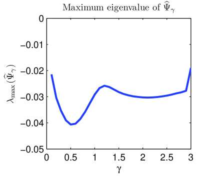
By Theorem 1, a valid $\gamma$-ICA procedure must correspond to $\Psi_{\gamma}<0$, or equivalently, the maximum eigenvalue of $\Psi_{\gamma}$, denoted by $\lambda_{\max}(\Psi_{\gamma})$, must be negative. How should one pick a $\Gamma$-interval so that $\gamma\in\Gamma$ is legitimate in the sense that $\lambda_{\max}(\Psi_{\gamma})<0$? Our suggestion for a rule of thumb is as follows. Let $\widehat{\Psi}_{\gamma}$ be the empirical estimator of $\Psi_{\gamma}$ based on the estimated source $\{\widehat{s}_{i}\}_{i=1}^{n}$, where $\widehat{s}_{i}:=\widehat{W}^{\top}z_{i}$. The plot of $\{(\gamma,\lambda_{\max}(\widehat{\Psi}_{\gamma}))\}$ then provides a guidance in determining $\Gamma$, over which $\lambda_{\max}(\widehat{\Psi}_{\gamma})$ should be far away below zero. With the $\Gamma$-interval, a further selection procedure, introduced in Section 5, can be applied to select an optimal $\gamma$ value from $\Gamma$. It is confirmed in our numerical study in Section 6 that, the interval $\Gamma$, where $\lambda_{\max}(\widehat{\Psi}_{\gamma})<0$, is quite wide, and the suggested rule does provide adequate choice of $\Gamma$. It also implies that the choice of $\tau$ in Corollary 2 is not critical, as $\tau$ is allowed to vary in a wide range and not limited to very small number. It is the condition (B) that plays the most important role to ensure the recovery consistency of $\gamma$-ICA.

3.4 $\beta$-ICA versus $\bm{\gamma}$-ICA

By using $\beta$-divergence, Mihoko and Eguchi (2002) proposed $\beta$-ICA to recover independent components. The objective function of $\beta$-ICA being maximized is of the form

$$|{\rm det}(W)|^{\beta}\left\{\int f^{\beta}(W^{\top}z)g_{Z}(z)dz-c_{\beta}\right\},$$ (33)

where $c_{\beta}$ is a known constant. If we restrict $W\in{\cal SO}_{p}$, then $|{\rm det}(W)|=1$ and maximizing (33) is equivalent to maximizing $\int f^{\beta}(W^{\top}z)g_{Z}(z)dx$, which has the same form with the population objective function of $\gamma$-ICA in (28). We should emphasize that Mihoko and Eguchi (2002) considered the ICA problem under the original $X$-scale, while the constraint $W\in{\cal SO}_{p}$ is a consequence of prewhitening. Without considering the constraint $W\in{\cal SO}_{p}$, the objective function of $\gamma$-ICA is deduced to be

$$|{\rm det}(W)|^{\frac{\gamma}{\gamma+1}}\left\{\int f^{\gamma}(W^{\top}z)g_{Z}(z)dz\right\}$$ (34)

which is different from (33). However, (33) is similar to (34) when $c_{\beta}$ is small. This fact also confirms the observation of Mihoko and Eguchi (2002) that setting $c_{\beta}=0$ does not affect the performance of $\beta$-ICA. In summary, $\gamma$-ICA and $\beta$-ICA based on the whitened data $Z$ are equivalent. For data $X$ in original scale, however, $\gamma$-ICA maximizing (34) is different from $\beta$-ICA maximizing (33), but they will have similar performance for small $\beta$.

4 Gradient method for $\bm{\gamma}$-ICA on $\bm{{\cal SO}_{p}}$

In this section, we introduce an algorithm for estimating $W$ constrained to the special orthogonal group ${\cal SO}_{p}$, which is a Lie group and is endowed with a manifold structure. The Lie group ${\cal SO}_{p}$, which is a path-connected subgroup of $\mathcal{O}_{p}$, consists of all orthogonal matrices in $\mathbb{R}^{p\times p}$ with determinant one. Recall $\mathcal{L}$ being the objective function of $\gamma$-ICA maximization problem defined in (28). A desirable algorithm is to generate an increasing sequence $\{\mathcal{L}(W_{k})\}_{k=1}^{\infty}$ with $W_{k}\in{\cal SO}_{p}$, such that $\{W_{k}\}_{k=1}^{\infty}$ converges to a local maximizer $W^{*}$ of $\mathcal{L}$. Various approaches can be used to generate such a sequence $\{W_{k}\}_{k=1}^{\infty}$ in ${\cal SO}_{p}$, for instance, geodesic flows and quasi-geodesic flows (Nishimori and Akaho, 2005). Here we focus on geodesic flows on ${\cal SO}_{p}$. In particular, starting with the current $W_{k}$, the update $W_{k+1}$ is selected from one geodesic path of $W_{k}$ along the steepest ascent direction such that $\mathcal{L}(W_{k+1})>\mathcal{L}(W_{k})$. In fact, this approach has been applied to the general Stiefel manifold (Nishimori and Akaho, 2005). Below we briefly review the idea and then introduce our implementation algorithm for $\gamma$-ICA. We note that the proposed algorithm is also applicable to MLE-ICA by changing the corresponding objective function.

Let $T_{W}{\cal SO}_{p}$ denote the tangent space of ${\cal SO}_{p}$ at $W$. Consider a smooth path $W(t)$ on ${\cal SO}_{p}$ with $W(0)=W$. Differentiating $W(t)^{\top}W(t)=I_{p}$ yields the tangent space at $W$

$$T_{W}{\cal SO}_{p}=\left\{WV:V\in\mathbb{R}^{p\times p},V^{\top}=-V\right\}.$$ (35)

Clearly, $T_{I_{p}}{\cal SO}_{p}$ is the set of all skew-symmetric matrices. Each geodesic path starting from $I_{p}$ has an intimate relation with the matrix exponential function. In fact, $\exp(V)\in{\cal SO}_{p}$ if and only if $V$ is skew-symmetric (see page 148 in Boothby, 1986; Proposition 9.2.5. in Marsden and Ratiu, 1998). Moreover, for any $M\in{\cal SO}_{p}$, there exists (not unique) a skew-symmetric $V$ such that $M=\exp(V)$. If the Killing metric (Nishimori and Akaho, 2005)

$$g_{W}(Y_{1},Y_{2}):={\rm tr}(Y_{1}^{\top}Y_{2}),\;\;{\rm where}~{}Y_{1},Y_{2}\in T_{W}{\cal SO}_{p},$$

is used, the geodesic path starting from $I_{p}$ in the direction $V$ is given by

$$\left\{\Phi(V,t):~{}t\in\mathbb{R}\right\}\quad{\rm with}\quad\Phi(V,t):=\exp(tV).$$ (36)

Since the Lie group is homogeneous, we can compute the gradient and geodesic at $W_{k}\in{\cal SO}_{p}$ by pulling them back to the identity $I_{p}$ and then transform back to $W_{k}$. In the implementation algorithm, to ensure all the iterations lying on the manifold ${\cal SO}_{p}$, we update $W_{k+1}$ through

$$W_{k+1}:=W_{k}\exp(t_{k}V_{k}),$$ (37)

where the skew-symmetric matrix $V_{k}$ and the step size $t_{k}$ are chosen properly to meet the ascending condition $\mathcal{L}(W_{k+1})>\mathcal{L}(W_{k})$. Since, from (36), $\exp(t_{k}V_{k})$ lies on the geodesic path of $I_{p}$, then $W_{k+1}=W_{k}\exp(t_{k}V_{k})$ must lie on the geodesic path of $W_{k}$. Moreover, since ${\rm det}(W_{k+1})={\rm det}(W_{k})\exp(0)=1$ by ${\rm tr}(V_{k})=0$, the sequence in (37) satisfies $W_{k}\in{\cal SO}_{p}$ for all $k$. The determination of the gradient direction $V_{k}$ and the step size $t_{k}$ is discussed below.

To compute the gradient and geodesic at $W_{k}$ by pulling them back to $I_{p}$, define

$$\mathcal{F}_{W_{k}}(W):=\mathcal{L}(W_{k}W).$$ (38)

We then determine $W_{k+1}=W_{k}\exp(t_{k}V_{k})$ from one geodesic at $I_{p}$ in the direction of the projected gradient of $\mathcal{F}_{W_{k}}$. Specifically, to ensure the ascending condition, we choose each skew-symmetric $V_{k}$ to be $\nabla_{{\!\!/\!/}}\mathcal{F}_{W_{k}}$, the projected gradient of $\mathcal{F}_{W_{k}}$ at $I_{p}$, defined to be

$$\nabla_{{\!\!/\!/}}\mathcal{F}_{W_{k}} := \mathop{\rm argmin}_{V\in T_{I_{p}}{\cal SO}_{p}}\|\nabla\mathcal{F}_{W_{k}}-V\|,\quad\mbox{where}~{}~{}\nabla\mathcal{F}_{W_{k}}:=\frac{\partial\mathcal{F}_{W_{k}}}{\partial W}\Big{|}_{W=I_{p}},$$ (39)

$$= \frac{1}{2}\left(\nabla\mathcal{F}_{W_{k}}-\nabla\mathcal{F}_{W_{k}}^{\top}\right)$$

$$= \frac{\gamma}{2n}\sum_{i=1}^{n}f^{\gamma}(W_{k}^{\top}z_{i})\left\{W_{k}^{\top}z_{i}\,\left[\phi(W_{k}^{\top}z_{i})\right]^{\top}-\phi(W_{k}^{\top}z_{i})\left[W_{k}^{\top}z_{i}\right]^{\top}\right\}.$$

This particular choice of $V_{k}$ ensures the existence of the step size $t_{k}$ for the ascending condition. Note that in the case of ${\cal SO}_{p}$ imposed with the Killing metric, the projected gradient coincides with the natural gradient introduced by Amari (1998). See also Fact 5 in Nishimori and Akaho (2005) for further details. As to the selection of the step size $t_{k}$ at each iteration $k$ with $W_{k}$ and $V_{k}=\nabla_{{\!\!/\!/}}\mathcal{F}_{W_{k}}$, we propose to select $t_{k}$ such that $W_{k}\exp(t_{k}V_{k})$ is the “first improved rotation”. In particular, we consider $t_{k}=\alpha\rho^{\ell_{k}}$ for some $\alpha>0$ and $0<\rho<1$, where $\ell_{k}$ is the nonnegative integer. To proceed, we search $\ell_{k}$ such that

$${\cal L}\big{(}W_{k}\exp(\alpha\rho^{\ell_{k}}V_{k})\big{)}>{\cal L}\big{(}W_{k}\big{)},\quad{\rm where}\quad V_{k}=\nabla_{{\!\!/\!/}}\mathcal{F}_{W_{k}},$$

and then update $W_{k+1}=W_{k}\exp(\alpha\rho^{\ell_{k}}V_{k})$. In our implementation, $\alpha=1$ and $\rho=0.5$ are used. For the convergence issue, one can instead consider the Armijo rule for $t_{k}$ (given in equation (40)). Our experiments show that the above “first improved rotation” rule works quite well. Lastly, in the implementation, to save the storage for $W_{k}$, we “rotate $\bm{Z}$ directly” instead of manipulating $W$, where $\bm{Z}$ is the $p\times n$ data matrix whose columns are $z_{i}$, $i=1,\dots,n$. That is, we use the update $\bm{Z}_{k}=W_{k}^{\top}\bm{Z}$. To retrieve the matrix $W$, we simply do a matrix right division of the final $\bm{Z}$ and the initial $\bm{Z}$. The algorithm for $\gamma$-ICA based on gradient ascend on ${\cal SO}_{p}$ is summarized below.

 

1. Initialization: $\alpha=1$, $\rho=0.5$, prewhitened data $\bm{Z}_{1}=\bm{Z}$ (${p\times n}$ matrix).

2. For each iteration $k=1,2,3,\ldots$,

   • Compute the skew-symmetric matrix $V_{k}$ in (39).

   • For $\ell_{k}=0,1,2,\ldots$, if $\mathcal{F}_{W_{k}}(\exp(\alpha\rho^{\ell_{k}}V_{k}))>{\cal F}_{W_{k}}(I_{p})$, then break the loop.

   • Update $\bm{Z}_{k+1}$ by $\exp(\alpha\rho^{\ell_{k}}V_{k})^{\top}\bm{Z}_{k}$. Check the convergence criterion. If the criterion is not met, go back to (i).

3. Output $\widehat{W}=\left(\bm{Z}_{1}\bm{Z}_{1}^{\top}\right)^{-1}\bm{Z}_{1}\bm{Z}_{k}^{\top}$.

  

Finally, we would like to mention the convergence issue. The statement is similar to Proposition 1.2.1 of Bertsekas (2003).

Theorem 5.

Let $\mathcal{L}$ be continuously differentiable on ${\cal SO}_{p}$, and $\mathcal{F}$ be defined in (38). Let $\{W_{k}\in{\cal SO}_{p}\}$ be a sequence generated by $W_{k+1}=W_{k}\exp(t_{k}V_{k})$, where $V_{k}$ is a projected gradient related (see (41) below) and $t_{k}$ is a properly chosen step size by the Armijo rule: reduce the step size $t_{k}=\alpha\rho^{\ell_{k}}$, $\ell_{k}=0,1,2,\ldots,$ until the inequality holds for the first nonnegative $\ell_{k}$,

$$\mathcal{L}(W_{k+1})-\mathcal{L}(W_{k})=\mathcal{F}_{W_{k}}(\exp(t_{k}V_{k}))-\mathcal{F}_{W_{k}}(I_{p})\geq\eta\,t_{k}\,{\rm tr}\left(\nabla_{\!\!/\!/}\mathcal{F}_{W_{k}}^{\top}V_{k}\right),$$ (40)

where $0<\eta<1$ is a fixed constant. Then, every limit point $W^{*}$ of $\{W_{k}\in{\cal SO}_{p}\}$ is a stationary point, i.e., ${\rm tr}(\nabla\mathcal{F}_{W^{*}}^{\top}V)=0$ for all $V\in T_{W^{*}}{\cal SO}_{p}$, or equivalently, $\nabla_{\!\!/\!/}\mathcal{F}_{W^{*}}=0$.

The statement that $V_{k}$ is a projected gradient related corresponds to the condition

$$\limsup_{k\to\infty}\,{\rm tr}\left(\nabla_{\!\!/\!/}\mathcal{F}_{W_{k}}^{\top}V_{k}\right)>0.$$ (41)

This condition is true when $V_{k}$ is the projected gradient $\nabla_{\!\!/\!/}\mathcal{F}_{W_{k}}$ itself or some natural gradient $M^{-1}\nabla_{\!\!/\!/}\mathcal{F}_{W_{k}}$ (Theorem 1, Amari, 1998), where $M$ is a Riemannian metric tensor, which is positive definite.

5 Selection of $\gamma$

The estimation process of $\gamma$-ICA consists of two steps: $\gamma$-prewhitening and the geometry-based estimation for $W$, in which the values of $\gamma$ are essential to have robust estimators. Hence, we carefully select the value of $\gamma$ based on the adaptive selection procedures proposed by Minami and Eguchi (2003) and Mollah et al. (2007). We first introduce a general idea and then apply the idea to the selection of $\gamma$ in both $\gamma$-prewhitening and $\gamma$-ICA. Define the measurement of generalization performance as

$$C_{\gamma_{0}}(\gamma)=E[\mathcal{D}_{\gamma_{0}}(g,f_{\widehat{\theta}_{\gamma}})],$$ (42)

where $g$ is the underlying true joint probability density function of the data, $f_{\theta}$ is the considered model for fitting, $\widehat{\theta}_{\gamma}:=\mathop{\rm argmin}_{\theta}\mathcal{D}_{\gamma}(\widehat{g},f_{\theta})$ is the minimum $\gamma$-divergence estimator of $\theta$, and $\widehat{g}$ is the empirical estimate of $g$. The $\gamma_{0}$ is called the anchor parameter and is fixed at $\gamma_{0}=1$ throughout this paper. This value is empirically shown to be insensitive to the resultant estimators (Minami and Eguchi, 2003). Let $\widehat{C}_{\gamma_{0}}(\gamma)$ be the sample analogue of $C_{\gamma_{0}}(\gamma)$. We propose to select the value of $\gamma$ over a predefined set $\Gamma$ through

$$\widehat{\gamma}=\mathop{\rm argmin}_{\gamma\in\Gamma}\widehat{C}_{\gamma_{0}}(\gamma).$$ (43)

For $\gamma$-prewhitening, $g=g_{X}$ and $f_{\theta}=\xi_{\mu,\Sigma}$ with $\theta=(\mu,\Sigma)$. For $\gamma$-ICA, $g=g_{Z}$ and $f_{\theta}=f_{Z}(\cdot;W)$ with $\theta=W$.

The above selection criterion requires the estimation of $C_{\gamma_{0}}(\gamma)$. To avoid the problem of overfitting, we apply a $K$-fold cross-validation. Let $\mathcal{T}$ be the whole data, and let $K$ partitions of $\mathcal{T}$ be $\mathcal{T}_{1},\ldots,\mathcal{T}_{K}$, that is, $\mathcal{T}_{i}\bigcap\mathcal{T}_{j}=\emptyset$ if $i\not=j$ and $\mathcal{T}=\cup_{i=1}^{K}\mathcal{T}_{i}$. The whole selection procedure is summarized below.

 

1. For $k=1,\ldots,K$,

   1. For every $\gamma\in\Gamma$, obtain $\widehat{\theta}_{\gamma}^{(-k)}:=\mathop{\rm argmin}_{\theta}C_{\gamma}(\widehat{g}^{(-k)},f_{\theta})$, where $\widehat{g}^{(-k)}$ is the empirical estimate of $g$ based on $\mathcal{T}\setminus\mathcal{T}_{k}$.

   2. Compute the cross validation estimate $C_{\gamma_{0}}(\widehat{g}^{(k)},f_{\widehat{\theta}_{\gamma}^{(-k)}})$, where $\widehat{g}^{(k)}$ is the empirical estimate of $g$ based on $\mathcal{T}_{k}$.

2. Estimate $C_{\gamma_{0}}(\gamma)$ by

   $$\widehat{C}_{\gamma_{0}}(\gamma)=\frac{1}{K}\sum_{k=1}^{K}C_{\gamma_{0}}(\widehat{g}^{(k)},f_{\widehat{\theta}_{\gamma}^{(-k)}})$$ (44)

   and obtain $\widehat{\gamma}=\mathop{\rm argmin}_{\gamma\in\Gamma}\widehat{C}_{\gamma_{0}}(\gamma)$.

 

Eventually, we have two optimal values of $\gamma$: $\widehat{\gamma}_{\mu,\Sigma}$ for $\gamma$-prewhitening and $\widehat{\gamma}_{W}$ for estimation of the recovering matrix $W$.

6 Numerical experiments

We conduct two numerical studies to demonstrate the robustness of the $\gamma$-ICA procedure. In the first study, the data is generated from independent sources with some known distributions. In the second study, we use transformations of Lena images to form mixed image.

6.1 Simulated data

We independently generate the two sources $S_{j}$, $j=1,2$, from a non-Gaussian distribution with sample size $n=150+n_{1}$. The observable $X$ is then given by $X=AS$, where

$$A=\left[\begin{array}[]{cc}1&2\\ 1&0.5\end{array}\right].$$

Among the $n$ observations, we add to each of the last $n_{1}$ observations a random noise $e$. The data thus contains $150$ uncontaminated i.i.d. observations from the ICA model, $X=AS$, and $n_{1}$ contaminated i.i.d. observations from $X=AS+e$, where $e\sim N(\mu,\sigma^{2}I_{2})$ with $\mu=(5,5)$ and $\sigma=5$. We consider two situations for the independent source $S=(S_{1},S_{2})$:

1. Uniform source: Each $S_{j}$, $j=1,2$, is generated from Uniform$(-3,3)$.

2. Student-$t$ source: Each $S_{j}$, $j=1,2$, is generated from $t$-distribution with 3 degrees of freedom.

For the case of uniform source, we use the sub-Gaussian model $f_{j}(s)\propto\exp(-cs^{4})$ with $c=0.1$, which ensures the variance under $f_{j}$ is close to unity. As to the case of $t$ source, the super-Gaussian model $f_{j}(s)\propto 1/{\rm cosh}(cs)$ is considered, and we follow the suggested range of Hyvärinen and Oja (2000) and set $c=1.5$. We also implement MLE-ICA (using the geometrical algorithm introduced in Section 4) and fast-ICA (using the code available at http://www.cis.hut.fi/projects/ica/fastica/) based on the $\gamma$-prewhitened data for fair comparisons. To evaluate the performance of each method, we modify from the performance index of Parmar and Unhelkar (2009) by a rescaling and by replacing the 2-norm with 1-norm and define the following performance index

$$\pi=\frac{1}{2p(p-1)}\sum_{i}\left\{\left(\frac{\sum_{k}|\pi_{ik}|}{\max_{j}|\pi_{ij}|}-1\right)+\left(\frac{\sum_{k}|\pi_{ki}|}{\max_{j}|\pi_{ji}|}-1\right)\right\}\leq 1,$$ (46)

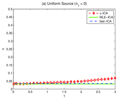
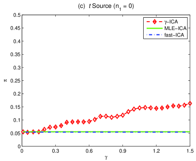
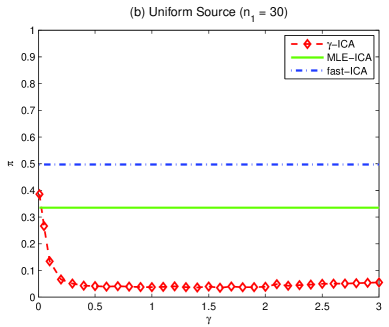
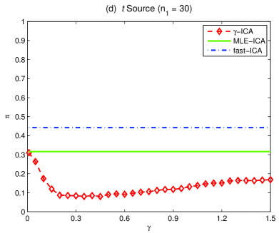
where $\pi_{ij}$ is the $(i,j)$-th element of $\Pi=\widetilde{A}\,\widehat{W}^{\top}$. We will expect $\Pi$ to be a permutation matrix, when the method performs well. In that situation, the value of $\pi$ should be very close to 0, and attains $0$ if $\Pi$ is indeed a permutation matrix. Simulation results with 100 replications are reported in Figure 1.

For the case of no outliers ($n_{1}=0$), all three methods perform well except the performance index $\pi$ of $\gamma$-ICA increases as $\gamma$ increases. This is reasonable since, according to Theorem 1, $\gamma$-ICA may fail to apply when $\gamma$ is too large. However, this influence is not severe as the the performance index $\pi$ is slightly increased only. As to the case of involving outliers ($n_{1}=30$), it can be seen that the proposed $\gamma$-prewhitening followed by $\gamma$-ICA does possess the advantage of robustness for a wide range of $\gamma$ values, while the other two methods are not able to recover the latent sources. The performance of $\gamma$-ICA becomes worse when $\gamma$ is small, since in the limiting case $\gamma\to 0$, $\gamma$-ICA reduces to the non-robust MLE-ICA. We note that both $\gamma$-prewhitening and $\gamma$-ICA are critical. This can be seen from the poor performance of MLE-ICA and fast-ICA, even they use the $\gamma$-prewhitened data as the input. Indeed, $\gamma$-prewhitening only ensures that we shift and rotate the data in a robust manner, while the outliers will still enter into the subsequent estimation process and, hence, a non-robust result is expected. In Figure 2 we report the scatter plots of the recovered sources $\widehat{A}^{-1}X$ from each method, of $X$, and of $A^{-1}X$ for one simulation run ($n_{1}=30$). These plots still convey the same message that $\gamma$-ICA is the winner among three methods, where the pattern of the reconstructed sources from $\gamma$-ICA is the most close to that of $A^{-1}X$.

6.2 Lena image

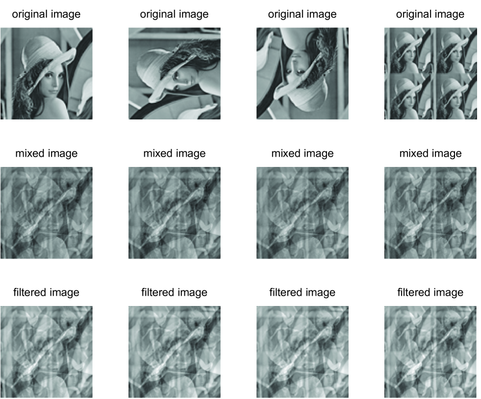
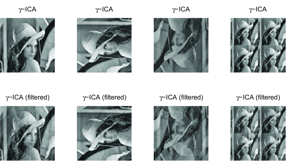
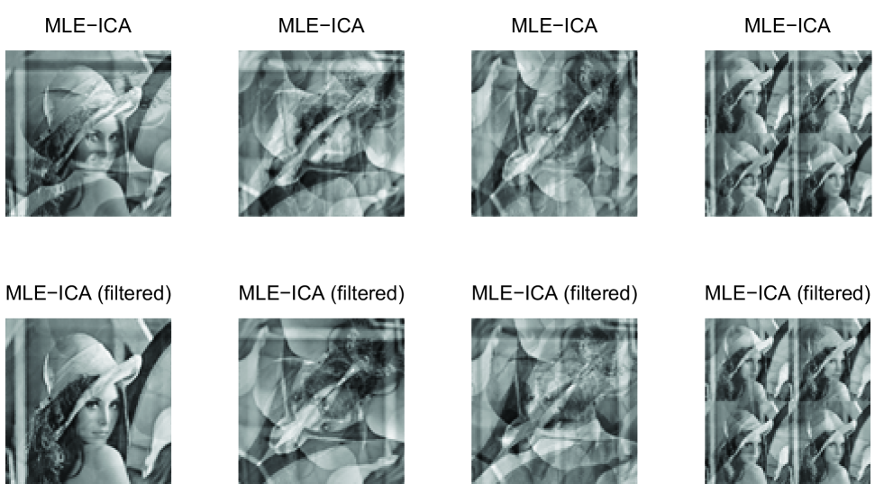
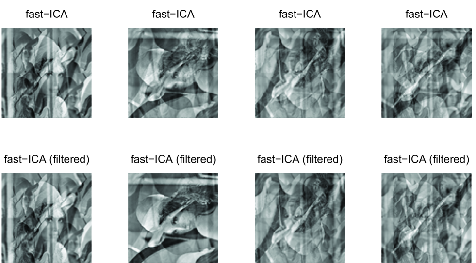
We use the Lena picture to evaluate the performance of $\gamma$-ICA. In our experiment, we use the Lena image with $512\times 512$ pixels. We construct four types of Lena as the latent independent sources $S$ as shown in Figure 5. We randomly generate the mixing matrix to be $A=1_{4}1_{4}^{T}+C$, where the elements of $C\in\mathbb{R}^{4\times 4}$ are independently generated from Uniform$(-0.3,0.3)$. The observed mixed pictures are also placed in Figure 5, wherein about $30\%$ of the pixels are added with random noise generated from $N(20,50^{2})$ for contamination. The aim of this data analysis is to recover the original Lena pictures based on the observed contaminated mixed pictures. In this analysis, the pixels are treated as the random sample, each with dimension 4. We randomly select $1000$ pixels to estimate the demixing matrix, and then apply it to reconstruct the whole source pictures. We conduct two scenarios to evaluate the robustness of each method:

1. Using the original image $X$ as the input (see the second row of Figure 5).

2. Using the filtered image $X^{*}$ from $X$ as the input (see the third row of Figure 5).

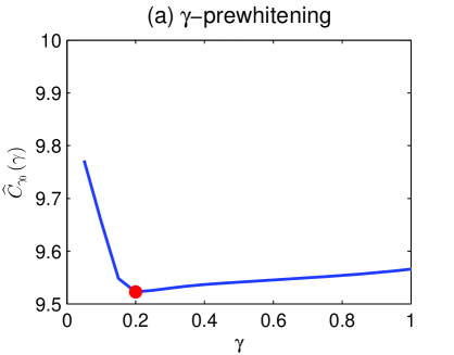
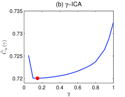
The filtering process in the second scenario can be treated as a pre-processing to alleviate the influence of additive Gaussian noise. In both scenarios, the estimated demixing matrix is applied to the original images $X$ to recover $S$. Note that with Gaussian noise contamination, conventional prewhitening by empirical moment estimators is not robust and, hence, both fast-ICA and MLE-ICA may fail to apply. Therefore, we prewhiten the data by $\gamma$-prewhitening first and then apply $\gamma$-ICA, MLE-ICA, and fast-ICA to the same whitened data for fair comparison. The plot $\{(\gamma,\lambda_{\max}(\widehat{\Psi}_{\gamma}))\}$ introduced in the end of Section 3.3 is placed in Figure 3, which suggests that $\Gamma=(0,1]$ is a good candidate for possible $\gamma$ values. We then apply the cross-validation method developed in Section 5 to determine the optimal $\gamma\in\Gamma$. The estimated values of $\widehat{C}_{\gamma_{0}}(\gamma)$ are plotted in Figure 4, from which we select $\widehat{\gamma}_{\mu,\Sigma}=0.2$ for $\gamma$-prewhitening and $\widehat{\gamma}_{W}=0.15$ for $\gamma$-ICA. The recovered pictures are placed in Figures 6-8, where for each figure the first row is for Scenario-1 and the second row is for Scenario-2.

It can be seen that $\gamma$-ICA is the best performer under both scenarios, while MLE-ICA and fast-ICA cannot recover the source images well when data is contaminated. It also demonstrates the applicability of the proposed $\gamma$-selection procedure. We detect that MLE-ICA and fast-ICA perform better when using filtered images $X^{*}$, but can still not reconstruct images as good as $\gamma$-ICA does. Interestingly, $\gamma$-ICA has a reverse performance, where the best reconstructed images are from the original images instead of the filtered ones. The filtering process, which aims to achieve robustness, replaces the original pixel value by the median of the pixel values over its neighborhood. Therefore, while filtering process will alleviate the influence of outlier, it is also possible to lose useful information at the same time. For instance, a pixel without being contaminated will still be replaced by certain median value during the filtering process. $\gamma$-ICA, however, works on the original data $X$ that possesses all the information available, and then weights each pixel according to its observed value to achieve robustness. Hence, a better performance for $\gamma$-ICA based on the original images is reasonably expected.

7 Conclusions

In this paper, we introduce a unified estimation framework by means of minimum $U$-divergence. For the reason of robustness consideration, we further focus on the specific choice of $\gamma$-divergence, which gives the proposed $\gamma$-ICA inference procedure. Statistical properties are rigorously investigated. A geometrical algorithm based on gradient flows on orthogonal group is introduced to implement our $\gamma$-ICA. The performance of $\gamma$-ICA is evaluated through synthetic and real data examples.

There are still many important issues that are not covered by this work. For example, we only consider full ICA problem, i.e., simultaneous extraction of all $p$ independent components, which is unpractical in the case of large $p$. It is of interest to extend our current $\gamma$-ICA to partial $\gamma$-ICA. Another issue of interest is also related to the large-$p$-small-$n$ scenario. In this work, data have to be prewhitened before entering the $\gamma$-ICA procedure. Prewhitening can be very unstable especially when $p$ is large. How to avoid such a difficulty is an interesting and challenging issue. Tensor data analysis is now becoming popular and attracts the attention of many researchers. Many statistical methods include ICA have been extended to deal with such a data structure by means of multilinear algebra techniques. An extension of $\gamma$-ICA to a multilinear setting to cover tensor data analysis is also of great interest for future study.

References

Amari, S., Chen, T. and Cichocki, A. (1997). Stability analysis of learning algorithms for blind source separation. Neural Networks, 10, 1345-1351.

Amari, S. (1998). Natural gradient works efficiently in learning. Neural Computation, 10, 251-276.

Basu, A., Harris, I. R., Hjort, N. L. and Jones, M. C. (1998). Robust and efficient estimation by minimizing a density power divergence. Biometrika 85, 549-559.

Bertsekas, D. P. (2003). Nonlinear Programming. Athena Scientific, Belmont, Massachusetts.

Boothby, W. M. (1986). An Introduction to Differentiable Manifolds and Riemannian Geometry. Academic Press.

Edelman, A., Aris, T. A. and Smith, S. (1998). The geometry of algorithm with orthogonality constraints SIAM J. Matrix Anal. Appl. 20, 303-353.

Eguchi, S. (2009). Information divergence geometry and the application to statistical machine learning. In Information Theory and Statistical Learning, F. Emmert-Streib and M. Dehmer (eds.), 309-332. Springer, Berlin.

Fiori, S. (2005). Quasi-geodesic neural learning algorithm over the orthogonal group: a tutorial. J. Machine Learning Research, 6, 743-781.

Fujisawa, H. and Eguchi, S. (2008). Robust parameter estimation with a small bias against heavy contamination. Journal of Multivariate Analysis, 99, 2053-2081.

Horn, R. A. and Johnson, C. R. (1991). Topics in Matrix Analysis. Cambridge University Press, Cambridge; New York.

Hyvärinen, A. (1998). New approximations of differential entropy for independent component analysis and projection pursuit. Advances in Neural Information Processing Systems, 10, 273-279.

Hyvärinen, A. (1999). Fast and robust fixed-point algorithms for independent component analysis. IEEE Transactions on Neural Networks, 10, 626-634.

Hyvärinen, A. and Oja, E. (2000). Independent component analysis: algorithm and applications. Neural Networks, 13, 411-430.

Hyvärinen, A., Karhnen, J. and Oja, E. (2001). Independent Component Analysis. Wiley Inter-Science.

Magnus, J. R. and Neudecker, H. (1979). The commutation matrix: some properties and applications. Annals of Statistics, 7, 381–394.

Marsden, J. E. and Ratiu, S. T. (1998). Introduction to Mechanics and Symmetry: A Basic Exposition of Classical Mechanical Systems. Springer.

Mihoko, M. and Eguchi, S. (2002). Robust blind source separation by $\beta$-divergence. Neural Computation, 14, 1859-1886.

Minami, M. and Eguchi, S. (2003). Adaptive selection for minimum $\beta$-divergence method. Proceedings of ICA-2003 Conference, Nara, Japan.

Mollah, M. N. H., Eguchi, S. and Minami, M. (2007). Robust prewhitening for ICA by minimizing $\beta$-divergence and its application to fastICA. J. Neural Processing Letters, 25, 91-110.

Murata, N., Takenouchi, T., Kanamori, T. and Eguchi, S. (2004). Information geometry of U-boost and Bregman divergence. Neural Computation, 16, 1437-1481.

Nishimori, Y. and Akaho, S. (2005). Learning algorithms utilizing quasi-geodesic flows on the Stiefel manifold. Neurocomputing, 67, 106-135.

Parmar, S. D. and Unhelkar, B. (2009). Performance analysis of ICA algorithms against multiple-sources interference in biomedical systems. International Journal of Recent Trends in Engineering, 2, 19-21.

Figure 1: The averages of the performance index $\pi$ for different methods.

Figure 2: The scatter plots for the recovered independent components from different methods, for the observed signals $X$, and for the true sources $S$. In each plot, the red dots are observations without contamination, and the blue pluses are contaminated ones. (a)-(e): Uniform source (Scenario-1), (f)-(j): $t$ source (Scenario-2).

Figure 3: The maximum eigenvalue of $\widehat{\Psi}_{\gamma}$ in (30) at different $\gamma$ values for the Lena data analysis.

Figure 4: The cross-validation estimates $\widehat{C}_{\gamma_{0}}(\gamma)$ with $\gamma_{0}=1$ for (a) $\gamma$-prewhitening and (b) $\gamma$-ICA for the Lena data analysis. The red dot indicates the place where the minimum value is attained.

Figure 5: Four images of Lena (the first row), the mixed images with $30\%$ pixels being contaminated (the second row), and the filtered images from the mixed images (the third row).

Figure 6: Recovered Lena images from $\gamma$-ICA based on the mixed images (the first row) and the filtered images (the second row).

Figure 7: Recovered Lena images from MLE-ICA based on the mixed images (the first row) and the filtered images (the second row).

Figure 8: Recovered Lena images from fast-ICA based on the mixed images (the first row) and the filtered images (the second row).