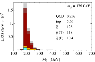
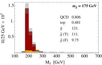
Boosted Multijet Resonances and New Color-Flow Variables
Abstract
We use modern jet-substructure techniques to propose LHC searches for multijet-resonance signals without leptons or missing energy. We focus on three-jet resonances produced by -parity-violating decays of boosted gluinos, showing that shape analyses searching for a mass peak can probe such gluinos up to masses of GeV (650 GeV) with () at the LHC at 8 TeV. This complements existing search strategies, which also include counting methods that are inherently more prone to systematic uncertainties. Since -parity-violating gluinos lighter than all squarks hadronize before decaying, we introduce new color-flow variables, “radial pull” and “axis contraction”, which are sensitive to the color structure of the -hadron’s decay. The former measures the inward pull of subjets in a fat jet, while the latter quantifies the inward drift of the -subjettiness axes when changing the distance measure. We show that they can dramatically improve the discrimination of a boosted gluino signal versus QCD, , and combinatoric background for . Cuts on axis contraction also noticeably improve the resonance shape for heavy gluinos with . With minor adaptations, these variables could find application in substructure searches for particles in different color representations or with other decay topologies. We also compare how several different Monte Carlo generators model the high-multiplicity QCD background. This provides evidence that the discriminating power of our color-flow observables are robust, and provides useful guidance for future substructure studies.
I Introduction
The Large Hadron Collider (LHC) is setting ever-more stringent constraints on many Beyond-Standard Model (BSM) theories. The most constrained BSM theories are those that produce large amounts of missing transverse energy (MET) and/or leptons ATLASnote:2012a ; 2012mfa ; ATLASnote:2012b ; CMSnote:2011b ; 2012ar ; CMSnote:2011c ; Chatrchyan:2012sa ; Aad:2011cw ; 2012he . However, there are many theories that do not feature these signatures. One of the more experimentally challenging signals are jets Sterman:1977wj with no MET or leptons, for which the background from ordinary Quantum Chromodynamics (QCD) processes is prodigious.
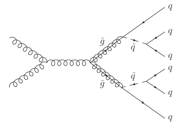
The particular signal that we study in this paper can be phrased in terms of a simplified model. In addition to the Standard Model particle content, we consider a colored particle that is pair-produced and decays to three light-flavored quarks Chivukula:1990di ; Chivukula:1991zk ; Farhi:1979zx ; Marciano:1980zf ; Frampton:1987ut ; Frampton:1987dn ; rouventhesis 111We leave decays to heavy-flavored quarks, which are in principle easier to detect, to future work.. A useful benchmark model for this scenario is the Minimal Supersymmetric (SUSY) Standard Model with baryon-number violating -parity violation (RPV) RPVoriginal ; RPVreview and a gluino as the lightest supersymmetric particle (LSP): the colored particles are gluinos, which each decay to a quark and an off-shell squark that decays to two quarks via an RPV coupling (see Fig. 1). This leads to a six-jet signal, with two three-jet resonances from the two decaying gluinos.
For other examples of multi-jet searches, see Alwall:2008ve ; Kilic:2008pm ; Kilic:2010et ; Alves:2011wf ; Tavares:2011zg ; Gross:2012bz ; Hook:2012fd .
If leptons and neutrinos appear in RPV cascade decays, bounds on superpartner masses can still be TeV rpvmsugra . However, the bounds are weaker if the signal is entirely hadronic, which we consider here. In particular, for a gluino LSP decaying to three jets, a model-independent bound on exotic color octets from LEP excludes gluino masses below 51 GeV LEPrpvgluinobound , while searches at CDF and CMS have only excluded gluinos with masses in the range GeV TEVATRONrpvgluinobound , GeV CMSrpvgluinobound36 , and GeV CMSrpvgluinobound5 . A recent ATLAS search has closed the gap between GeV and excludes gluinos up to 660 GeV ATLASrpvgluinobound5 . The weakened bounds relative to -parity-conserving SUSY make RPV an attractive possibility for natural SUSY models Allanach:2012vj ; Brust:2011tb ; Brust:2012uf ; Evans:2012bf .
The six-jet signal is challenging to see due to the large QCD background. A further difficulty is the large combinatorial ambiguity in correctly identifying the three jets from each gluino. The method in rouventhesis ; TEVATRONrpvgluinobound ; CMSrpvgluinobound36 ; CMSrpvgluinobound5 uses a correlation between the sum of the transverse momentum () and the invariant mass () of three jets to select a phase space region with a high number of signal relative to combinatorial and QCD background events. Even so often ends up being very small, motivating the investigation of complementary analysis methods.
The ATLAS study ATLASrpvgluinobound5 exploits the fact that the jets from gluino decays tend to have similar , while QCD six-jet events exhibit a hierarchy. Counting the number of events on the high-end tail of the sixth-hardest-jet- distribution excludes RPV gluinos up to 660 GeV ATLASrpvgluinobound5 , but does require an extremely reliable understanding of the background normalization. It is thus desirable to cross-check this result using an orthogonal search channel with a nearly independent set of systematic uncertainties (as also suggested in ATLASrpvgluinobound5 ).
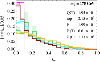
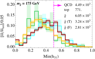
This motivates the focus of our paper: we examine the decay and radiation pattern produced by two boosted gluinos, whose decay products tend to be collimated and fall into the same region of the detector, producing two hard fat jets. The study of boosted gluinos allows for a reconstruction of in the fat-jet invariant mass distribution, giving a cleaner and more robust signal than other methods, and allowing a shape analysis to extract the gluino mass peak. We study boosted gluinos using jet-substructure techniques nsubjettiness ; Stewart:2010tn ; nsubjettinessminaxes ; pull ; Bassetto:1984ik ; dipolarity ; girth ; WtagRcores ; quarkgluontag ; planarflowtoptag ; BDRStagger ; jetpruning ; filteringfortag ; trimming ; filterforhiggs ; YsplitterATLAS ; Soper:2011cr ; Butterworth:2007ke ; Almeida:2010pa ; Jankowiak:2011qa ; Ellis:2012sn ; Butterworth:2002tt ; Jankowiak:2012na ; Salam:2009jx ; TWtoptagger ; Hopkinstoptagger , which have matured enormously in recent years and are being verified experimentally ATLASnote:2012a ; ATLASnote:2012b ; CMSnote:2011b ; CMSnote:2011c ; Abazov:2011vh ; ATLASsubstructurecomparison ; Aad:2011kq ; Aad:2012jf ; CMSnote:2011a ; Aaltonen:2011pg ; ATLASnote:2011a ; Chatrchyan:2012zt ; Seymour:1993mx (for some recent reviews see boost2010 ; toptagreview ; boost2011 ). We achieve the best signal sensitivity using -subjettiness nsubjettiness ; nsubjettinessminaxes to isolate three-pronged fat jets, requiring two high- fat jets with similar masses, and vetoing events with a large sub-jet -hierarchy. In addition, we introduce two new color-flow variables, radial pull and axis contraction. Radial pull is based on the pull variable defined in pull , while axis contraction exploits the shift in the minimizing axes of -subjettiness when changing the distance measure. Both variables help distinguish the signal’s QCD radiation pattern when compared with the QCD background. The background radiation pattern has been simulated with several Monte Carlo programs.
The ATLAS study ATLASrpvgluinobound5 examined boosted gluinos and excluded GeV (light compared to ), but we show that a boosted search is viable at the 8 TeV LHC (LHC8) up to GeV, where pb and the boosted fraction is only (few %). This shows that looking for relatively heavy gluinos in the boosted regime, first proposed for the Tevatron tevatronboostedgluinos , carries over to the LHC in spite of the smaller boosted fraction and production cross section of a collider relative to a collider. We also define a search for top-mass gluinos () with spectacular background discrimination that would improve on the ATLAS limit. This is relevant for other simplified models.
The new variables, radial pull and axis contraction, are designed to measure the distribution of the soft QCD radiation pattern inside each boosted-gluino fat jet. They should generalize to other examples of boosted jet studies futurework , for example hadronic RPV decays of neutralino LSPs (as in Butterworth:2009qa ). Their use in our study relies on the fact that gluinos decaying via an off-shell squark generically live longer than the hadronization time-scale, so that they form a color-singlet -hadron before decaying. This leaves a measurable soft QCD radiation pattern within each boosted fat jet, which differs from a beam-connected color octet like that for an un-hadronized gluino, combinatorics background, a boosted hadronic top quark, or QCD background. This effect of color-connected jets has been previously studied for a color singlet (such as or ) decaying into two jets forming a color dipole Bassetto:1984ik ; Bjorken:1991xr ; Bjorken:1992er ; Fletcher:1993ij ; Barger:1994zq ; pull ; dipolarity ; girth , and Tevatron experimental results demonstrated its viability Abazov:2011vh ; however, color flow has to our knowledge never been investigated for decaying -hadrons or non-dipole configurations.
In §II, we discuss the color flow in the gluino -hadron decay and introduce variables sensitive to the radiation pattern. §III describes our Monte Carlo (MC) generation; §IV details the substructure variables that distinguish boosted gluino decays from background, and show the results for searches for heavy ( GeV) and top-mass gluinos. §V contains our conclusions. A brief review of RPV gluinos is in Appenix A. A detailed Monte Carlo comparison for the QCD background of substructure and color-flow observables is described in Appendix B to ensure robustness of our results.
II Novel probes of color flow
 |
| (a) |
 |
| (b) |
 |
| (c) |
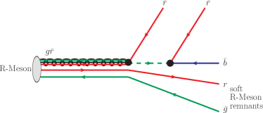
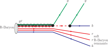
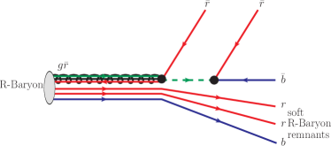
Gluinos that decay to three quarks through an off-shell squark and the baryon-violating RPV coupling (which appears in the superpotential as ) generically have a lifetime that is prompt but longer than the hadronization scale — see review in Appendix A. (We do not consider gluino decays originating from a displaced vertex or occurring outside the detector.) This means they first form color-singlet -hadrons before decaying to three jets. The pattern produced by the radiation from these signal jets is different from QCD background jets or from jets that originate from a particle that is a color fundamental (like a top quark) or octet (like an un-hadronized gluino decaying to three jets). In this section, we first give an intuitive explanation for the radiation pattern before introducing two new variables, radial pull and axis contraction, that attempt to quantify this. The new variables should, with slight adaptations, also be useful to distinguish background jets from jets originating from other particles like the Higgs or -boson, which we study elsewhere futurework .
II.1 Color Connections in -hadron Decays
The soft radiation pattern of a jet produced during hadronization will depend on how the color of the parent quark or gluon is connected to the color of the other quarks or gluons in the event. Put simply, the radiation pattern of a jet will be, on average, slightly ‘pulled’ towards other jets (or the beam) to which it is color-connected. Furthermore, gluons have a larger color charge than quarks and will produce on average a somewhat wider radiation pattern. A number of variables make use of this to, for example, tag dipole-pairs of jets and distinguish quarks from gluons WtagRcores ; dipolarity ; pull ; girth ; quarkgluontag .
The color flow of gluino pair production is identical to that of gluon pair production, with gluinos being color-connected to the proton remnants in the beam. Therefore, if the gluinos were stable, we would expect the -hadrons to be surrounded by a soft radiation pattern not unlike that of gluon jets. However, for decaying -hadrons the situation is more interesting. Fig. 2 shows the color flow of a decaying -meson and -baryon . Of the three hard jets from the decaying -meson, one forms a ‘mesonic’ singlet with one of the -meson remnant spectator quarks, while two form a ‘baryonic’ singlet with the other one of remnant quarks (a similar pattern of color connection with the remnants holds for decaying gluinoballs ). For -baryons, there are two distinct possibilities: two baryonic singlets, one formed out of one hard jet and two spectators and the other formed out of two hard jets and one spectator; or three mesonic singlets incorporating one hard quark each.
|
|
|
|
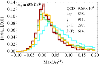
Right: Same as plot on left, but now showing the normalized distribution of the new color-flow variable axis-contraction ( with ) for GeV. An equivalent set of cuts has been applied, same as for Fig. 7 (a). In both cases the distribution of the good signal events differs markedly from the other (background) distributions.
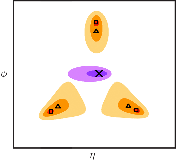
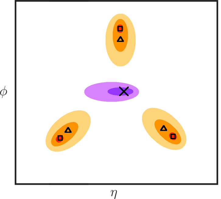
The resulting soft radiation pattern expected in the decay of a boosted -hadron is shown in strongly exaggerated schematic form in Fig. 3. The soft radiation field (purple region) of the first round of hadronization (during -hadron formation) is contained in the center of the fat jet, and might contain evidence of the initial gluino’s color connection to the beam, indicated here by its left-ward slant. However, this radiation field is extremely soft, as well as subject to the possible shortcomings of -hadronization models, and it will not be our focus. Superimposed on this initial radiation field is the result of the -hadron decay, and a second round of hadronization to resolve the color connections amongst its decay products. It is in the radiation fields of the three hard subjets of the fat jet that it may be possible to find evidence of the overall singlet nature of the -hadron: there should be an overall pull towards the center, and possibly between two fat jets that form a baryonic singlet with part of the remnant. While there is substantial overlap in the signal and background distributions of color-flow variables, we do find that aggressive cuts on color-flow variables that isolate events with the patterns shown in Fig. 3 are very helpful in improving signal-to-background ratios for RPV gluino searches. Any such variable can also be viewed as a generalization of existing dipole taggers, and could also find application elsewhere.
II.2 Radial Pull
The distribution of the radiation field of a jet can be measured with a variable called pull pull , defined as
| (1) |
where is a vector in the plane pointing from the jet axis to the jet constituent, and () is the transverse momentum of the jet ( jet constituent). The direction of the pull vector indicates an overall slant in the jet’s radiation distribution, while the magnitude contains limited information pull .
For a fat jet with subjets, we can calculate the pull vector for each subjet and combine them in a quantity that we call radial pull, defined as
| (2) |
where is the pull vector (normalized to unity) for the -th subjet and is the unit vector from the fat-jet center to the subjet axis, i.e. the difference between the subjet’s and fat-jet three-momentum vector, normalized to unity. By definition, .
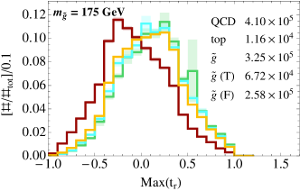
Radial pull characterizes the degrees to which a fat jet’s subjets are color-connected to the fat-jet center. Radial pull is expected to be closer to for the decay of a color-singlet -hadron located at the fat-jet center (see Fig. 3), whereas fat jets from QCD are expected to have components with color connections to the beam and other jets in the event, yielding a radial pull closer to . This is confirmed by MC simulations of the signal and background (in case of the background, with several different generators, see Section III and Appendix B). Fig. 4 (left) shows the normalized distribution of for a gluino with GeV (red and orange) and QCD (green) and (cyan) backgrounds (basic generator and trigger level cuts have been included). We divide the signal into two components: red (orange) in Fig. 4 corresponds to those events in which the hardest two fat jets line up (do not line up) within with the three-momentum of the two gluino -hadrons at the MC truth level. The red distribution is thus enriched with events where two fat jets originate from a decaying gluino, and thus constitute “good” (T) signal events. We see that the good signal events peak at values closer to and have a distinct distribution from the “bad” (F) signal events and from QCD and backgrounds.
We also tried an alternative definition of radial pull,
| (3) |
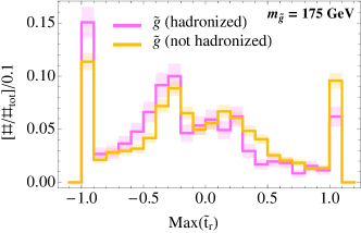
This variable is most sensitive to the dominant subjet pull, and so is peaked strongly at . We find that it works less well in distinguishing signal from background compared to the definition in Eq. (2). However, Eq. (3) is better at distinguishing radiation patterns from hadronized gluinos (-hadrons) vs. unhadronized gluinos. This is evident in Fig. 5, where a ratio between the +1 and -1 bin distinguishes clearly between decaying hadronized and un-hadronized gluinos. It is possible that for other types of signal Eq. (3) may be more useful, but in this paper, we use Eq. (2).
II.3 Axis Contraction
A second variable to measure the QCD radiation pattern of a boosted heavy particle exploits previously unexplored properties of -subjettiness, nsubjettiness , which we first review. is based on the variable -jettiness Stewart:2010tn , and is the average of the ’s of jet-constituent particles, weighted by the distance to a set of axes,
| (4) | |||||
| (5) |
where is the fat-jet radius and the sum is over all jet constituents . characterizes how well the radiation in the jet is aligned along these chosen axes, which are labelled by . is the distance in the plane between axis and constituent , and the axes are chosen in each instance to minimize the value of nsubjettinessminaxes unless indicated otherwise. (This is implemented in the FastJet -subjettiness plug-in nsubjettinessminaxes and provides substantially better discriminating power in boosted particle taggers than when the -subjettiness axes are chosen using a traditional jet clustering algorithm such as anti-) nsubjettiness .) determines the weighting in the sum of radiation far from the axes; typically .
By comparing values of for different , it is possible to characterize the number of subjets in the event. For example, if , the radiation in the jet is clustered around two separate axes within the jet, implying that the jet contains two prominent subjets. By contrast, if , then the radiation is distributed fairly evenly around the central jet axis and is not well characterized by two subjets. The ratio is useful for tagging jets from the decay of a boosted -boson, whereas the ratio can isolate jets with three distinct subjets, which is useful to tag boosted top quarks boost2010 ; boost2011 ; nsubjettiness ; nsubjettinessminaxes as well as boosted RPV gluino decays, as we show below.
Varying the parameter changes the sensitivity of to radiation far from the -subjettiness axes, and can therefore probe the shape of the radiation inside the fat jet. This provides a sensitivity not just to the number of ‘hard subjet-like structures’ in a fat jet (which might be accessed by reclustering) but also to the shape of their radiation patterns. Traditionally, this has been exploited in top-taggers nsubjettiness ; nsubjettinessminaxes by setting to make -subjettiness hone in on very tight radiation centers.
A novel way of exploiting this shape sensitivity is to study the -variance of the axes which minimize . (The idea of varying the parameters of event shape variables to extract additional information was first proposed in georgeeventshape .) Consider a fat jet with well-defined subjets. We denote the axes which minimize by
| (6) |
If the soft radiation field of a subjet associated with axis is skewed towards one side, then the axis is shifted away from the center of the subjet, and this shift is more pronounced for higher values of . Therefore, for example, the vector
| (7) |
which we call axis pull, should point in the direction of the skew for . This typically points in the same direction as the pull (1).
For the radiation pattern from gluinos, shown in Fig. 3, the skew of the radiation field should lie between the subjet axis and the fat jet center. To capture this effect, we define a scalar quantity called axis contraction as
| (8) |
where marks the fat jet centroid, i.e. the fat jet momentum in the plane, and . For our application we choose .
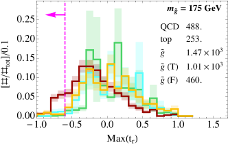
If the axes shift towards (away) from the centroid of the fat jet as is changed from 1 to 2, then is smaller (larger) than 0. We therefore expect that for boosted RPV gluinos, is on average smaller for signal fat jets that contain all of a gluino’s decay products than for fat jets from kinematically identical QCD or backgrounds, or signal fat jets that do not contain the decay products of a single gluino. This is again confirmed by MC simulations of the signal and background, which are described in detail in §III. For light gluinos, axis contraction performs comparably to radial pull, though the latter does have slightly better discrimination power. However, axis contraction is more suitable when cutting conservatively and wanting to preserve the largest amount of signal, as opposed to achieving maximum signal purity. This makes it more suitable for the heavy gluino case. Fig. 4 (right) shows the normalized distributions of for a gluino with GeV (red and orange) and QCD (green) and (cyan) backgrounds (basic generator and trigger level cuts have been included). The discrimination power of the variable for this heavy gluinos becomes more apparent as additional cuts are applied, see Fig. 7(g).
Note that the small numerical range of the axis contraction variable over our event samples is not indicative of any unrealistic detector resolution required to observe its variation, but is just a matter of how the variable is normalized. Furthermore, the shapes of the jet- distributions are very different at maximal vs minimal values of axis contraction (or radial pull). These differences are easily distinguished by the calorimeter and particle tracker.
The idea of using a shift in the -subjettiness axes under a change of to probe color flow is very general. One could imagine using as a dipole tagger, for example. This will be investigated further in futurework .
III Monte Carlo Event Generation
We simulated gluino pair production, -hadron formation, and RPV decay with a developmental version of Pythia 8.165 pythia6manual ; pythia8RPV ; pythia6RPV ; pythia8 222We thank Torbjörn Sjöstrand and Peter Skands for their quick implementation in Pythia of a baryon-violating RPV decay after -hadron formation, and for supplying us with a developmental version of Pythia that included this feature. Their change is now implemented in the publicly available Pythia 8.170.. This was done for two ranges: “top-mass” gluinos with and heavy gluinos with . The number of unweighted signal events simulated for the heavy (light) gluino analysis was () per mass point. All distributions were reweighted to correspond to a given luminosity at LHC8, usually 20 . Samples without -hadron formation before the decay were also generated for comparison. All signal cross sections were calculated at NLO in Prospino prospino .
We used Sherpa 1.4.0 sherpa ; sherpaother to generate fully matched QCD (with 2-6 hard jets from the Leading-Order matrix element) and background samples (fully hadronic decays with additional hard jets), with additional jets produced by the shower. Event generation was weighted to adequately sample high-multiplicity and high- events. We generated separate backgrounds for the heavy and the top-mass gluino searches:
-
•
Heavy gluino ( GeV) search: The relevant trigger is GeV along with at least one jet of GeV private.communication.1 , while the analysis itself requires two hard fat jets. Accordingly, we required background events at generator level to have two fat jets (anti-, ) each with GeV, along with one thin jet (anti-, ) with GeV. All generator-level cuts act at parton-level, and thresholds are correspondingly conservative compared to later cuts on the fully showered event. Because efficiencies of subsequent cuts are low, we generated a sample of million QCD events and million events. We find that the dominant background by far is QCD. Top backgrounds have a much smaller cross section and tend to produce fat jets that lie around GeV, well below the gluino mass scale under study.
-
•
Top-mass gluino search: This search uses a trigger requiring six thin jets (anti-, ) with GeV for full efficiency. Therefore background events were required at generator level to have two fat jets (anti-, ) with GeV, as well as at least four thin jets with GeV. Nevertheless, the poor trigger and cut efficiencies required the generation of around 100 million QCD events. The top, for which we generated million events, is subdominant to QCD for most of our subsequent chain of cuts, but can dominate after the final color-flow cuts.
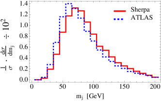
As a check of the backgrounds generated with Sherpa, we also considered backgrounds generated with independent matrix element generators and showering programs: POWHEG 1.0 + Pythia 6.4.27 and POWHEG 1.0 + Pythia 8.1.65 for QCD, and Madgraph 5.1.5 + Pythia 6.4.27 and Madgraph 5.1.5 + Pythia 8.1.65 for . The details of the MC comparison are in Appendix B. Overall, the different event generators are consistent with one another for jet-substructure and color-flow observables, although the tails of the distributions could differ in size by up to a factor of 10. Nevertheless, the broad conclusions of the efficacy of jet substructure and the discriminating power of color-flow observables are supported by all analyses. For the rest of this paper we compare the signal to backgrounds generated with Sherpa, since it is the only generator which provides fully matched event samples with up to 6 jets at matrix-element level as well as supporting weighted event generation to fully sample the tails of distributions. Ultimately, experimental study of color-flow observables will be needed to determine which MC program has the best agreement with data, but the comparison from Appendix B give a rough estimate of the dependence of generator effects on our observables. Because hadronization and RPV decay of gluinos is unique to Pythia 8, we were unfortunately unable to similarly estimate the generator-dependence of the signal observables.
All events are analyzed in our own FastJet 3.0.2 fastjet -based code, interfaced with the -subjettiness plugin nsubjettinessminaxes to calculate and find minimizing axes. Histograms were combined and reweighted in Mathematica to the number of expected events at LHC8 for a given integrated luminosity. For a histogram bin containing events with weight , the MC statistical error on the sum is , which we include in our distributions. We generated enough events to ensure that this statistical error is no larger than Poisson error corresponding to the actual expected number of LHC8 events, and that the distributions are as smooth as possible. Systematic errors are not included in our predictions, since the number of events surviving all the cuts is generally so small that Poisson uncertainties dominate. Detector effects are not explicitly modeled, but are unlikely to be a limiting factor since we only use the central part of the event (), our fat jets are extremely hard () and low statistics necessitate a large bin size for fat-jet-mass histograms anyway, precluding the use of any unrealistic mass resolution. Furthermore, as mentioned in the previous section, our color-flow variables do not rely on any unrealistic detector resolution to achieve their distinguishing power.
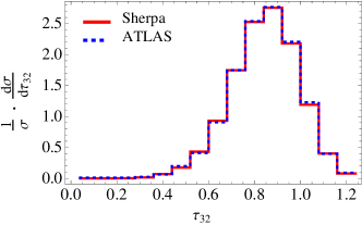
All signal and background samples include the underlying event and are generated using default parton distribution functions. To verify their validity, we applied several cross-checks to our background samples. We were able to reproduce the QCD 6-jet distributions from CMSrpvgluinobound36 as well as jet-mass and -subjettiness distributions from ATLASsubstructurecomparison (see Fig. 6). While the shape matched well across the entire range of all distributions (particularly for -subjettiness), the normalization was half as large as the data. Therefore, we scaled up the cross section of our entire QCD background sample (supplied at LO by Sherpa) by a -factor of 2. It was unnecessary to similarly re-scale the top background: it is negligible for the heavy gluino search, and while it is the dominant background after color cuts are applied in the top-mass gluino search, it is nevertheless eliminated by an additional -veto.
Only of top-mass gluinos and of heavy gluinos with a mass of are boosted enough for all the decay products to potentially end up in two fat jets. Since our search attempts to reconstruct a resonance in the fat jet mass spectrum, the large majority of signal events has to be treated as combinatorics background. Therefore, we divide the signal sample into two groups: “good” (T) signal, which is enriched with boosted gluinos by requiring that the two hardest fat jets are within of the truth-level gluinos, and “bad” (F) signal, i.e. the rest. This allows us to explicitly demonstrate that our cuts eliminate the QCD and as well as the combinatorics background.
IV Analysis
This section details our analysis strategy and results.
IV.1 Strategy
We discuss here the set of variables used to distinguish signal from background. Our aim is to remove as much QCD background as possible and have the gluino resonance be clearly distinguishable from the background. In particular, we do not rely on a counting analysis, as this is more susceptible to uncertainties in the background normalization.
In addition to the generator- and trigger-level cuts discussed in § III, we select events with the following properties:
-
1.
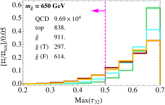
Two hard fat jets of size , clustered with the anti- algorithm Cacciari:2008gp . Each fat jet contains the three jets from a gluino decay if the gluino is boosted enough. We always consider only the two hardest fat jets in each event, and in many cases cut on the larger/smaller value of a variable evaluated for each jet (indicated with max/min).
-
2.
Each fat jet should be three-pronged. We use the N-subjettiness variable defined in Eq. (4) to select events with small values of
(9) -
3.
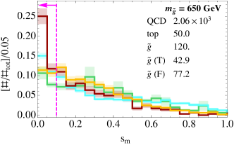
The two signal fat jets should have comparable invariant masses, since both reconstruct the gluino resonance. We thus select events with small values of the jet-mass symmetry parameter
(10) -
4.
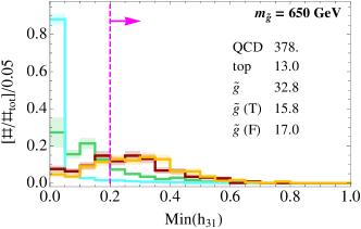
Each fat jet should contain three hard subjets with similar , since the QCD background jets tend to have asymmetric ’s. We thus select events where the subjet hierarchy parameter
(11) is close to one. Here is the -th subjet found by reclustering each fat jet constituents with anti-, . This variable is similar to the flow variable in Falkowski:2010hi . Versions of both and have been used in tevatronboostedgluinos .
-
5.
The radiation pattern within each fat jet should be that of a color-singlet -hadron. We thus select events with constraints on the new variables radial pull or axis contraction defined in Eqs. (2) and (8), respectively. For radial pull, we use subjets obtained by reclustering the fat-jet constituents with anti-, R = 0.4, the same as for .
We also evaluated other substructure variables like girth girth ; quarkgluontag and planar flow planarflowtoptag ; planarflow , but they did not add any discriminating power in our case.
IV.2 Pile-up Considerations & Effect of
Jet-Grooming
In the high luminosity environment of the LHC, the effects of pile-up (PU) can distort the spectrum of jet observables such as its mass and -subjettiness. The effects of pile-up can be largely eliminated using one of several jet-grooming techniques BDRStagger ; jetpruning ; filteringfortag ; trimming ; filterforhiggs ; Ellis:2009me . While we do not explicitly include the effects of jet-grooming in our main analysis, we verify here that an analysis based on variables outlined in §IV.1 give results that are applicable when jet grooming is included.
To see the effects of jet grooming, we trim trimming our samples by re-clustering fat jets into subjets of using the algorithm and discarding all subjets with . We take () for the heavy (top-mass) gluino analysis, with the precise value chosen to eliminate most of the effects of PU based on a simple model with mean PU energy of 12 GeV per unit area and intra-event fluctuations of 3 GeV per unit area (characteristic of PU with 20 primary vertices per event) pileupboost . We choose a smaller for heavier gluinos than for , since PU remains fixed even as the fat-jet increases for heavier gluinos. These parameters are comparable to those used by ATLASrpvgluinobound5 .
Trimming does alter the distributions of some of our kinematic variables; in particular, it tends to shift -subjettiness to lower values. However, we find that it is always possible to choose values of the cuts on , , and such that the overall signal and background efficiencies are essentially the same for trimmed and untrimmed samples, and so the outcomes of the ungroomed analyses remain the same when grooming is included. In fact, it is possible in some instances to achieve a background acceptance that is lower for the trimmed sample while maintaining the same signal efficiency; this makes our ungroomed analysis somewhat conservative, although we leave an optimization of jet grooming parameters to future work.
Our color-flow variables, however, must be calculated on the jets prior to grooming, because grooming can remove the soft radiation within and between subjets that distinguishes different color flows. To mitigate the effects of PU, it is preferable to include soft radiation over the smallest possible area. We find that, in most events, the values of the color-flow variables are dominated by radiation close to the subjet center, and we suggest that including only soft radiation within of each subjet axis would reduce contamination from PU (this is similar to the method of PU mitigation used in dipolarity ). Furthermore, we find that the scale of radiation driving the color-flow variables is GeV (and sometimes higher for heavy gluinos), which is above the characteristic scale of intra-event fluctuations in PU ( GeV for 20 primary vertices pileupboost ). We do not, however, include PU in our MC samples, and we leave it to the experimental collaborations to study precisely how color-flow variables are affected by PU and to confirm their utility.
| Common Cuts | Optimized Cuts | |||||||||||||||||||||||||||||
|---|---|---|---|---|---|---|---|---|---|---|---|---|---|---|---|---|---|---|---|---|---|---|---|---|---|---|---|---|---|---|
| Analysis |
generator level cuts |
Trigger: , |
two fat jets with |
|
|
|
|
fat jet |
axis contraction cut |
|||||||||||||||||||||
| QCD |
|
|
|
|
|
|
|
|
|
|||||||||||||||||||||
| top |
|
|
|
|
|
|
|
|
|
|||||||||||||||||||||
|
|
|
|
|
|
|
|
|
|
|||||||||||||||||||||
| QCD |
|
|
|
|
|
|
|
|
|
|||||||||||||||||||||
| top |
|
|
|
|
|
|
|
|
|
|||||||||||||||||||||
|
|
|
|
|
|
|
|
|
|
|||||||||||||||||||||
| QCD |
|
|
|
|
|
|
|
|
|
|||||||||||||||||||||
| top |
|
|
|
|
|
|
|
|
|
|||||||||||||||||||||
|
|
|
|
|
|
|
|
|
|
|||||||||||||||||||||
| QCD |
|
|
|
|
|
|
|
|
|
|||||||||||||||||||||
| top |
|
|
|
|
|
|
|
|
|
|||||||||||||||||||||
|
|
|
|
|
|
|
|
|
|
|||||||||||||||||||||
| QCD |
|
|
|
|
|
|
|
|
|
|||||||||||||||||||||
| top |
|
|
|
|
|
|
|
|
|
|||||||||||||||||||||
|
|
|
|
|
|
|
|
|
|
|||||||||||||||||||||
| QCD |
|
|
|
|
|
|
|
|
|
|||||||||||||||||||||
| top |
|
|
|
|
|
|
|
|
|
|||||||||||||||||||||
|
|
|
|
|
|
|
|
|
|
|||||||||||||||||||||
| QCD |
|
|
|
|
|
|
|
|
|
|||||||||||||||||||||
| top |
|
|
|
|
|
|
|
|
|
|||||||||||||||||||||
|
|
|
|
|
|
|
|
|
|
|||||||||||||||||||||
| QCD |
|
|
|
|
|
|
|
|
|
|||||||||||||||||||||
| top |
|
|
|
|
|
|
|
|
|
|||||||||||||||||||||
|
|
|
|
|
|
|
|
|
|
|||||||||||||||||||||
|
|
IV.3 Results for
|
|
| Analysis |
generator level cuts |
Trigger: 6 thin jets with |
two fat jets with |
|
|
|
|
radial pull cut |
-veto |
|||||||||||||||||||||||||||||||
|---|---|---|---|---|---|---|---|---|---|---|---|---|---|---|---|---|---|---|---|---|---|---|---|---|---|---|---|---|---|---|---|---|---|---|---|---|---|---|---|---|
| QCD |
|
|
|
|
|
|
|
|
|
|||||||||||||||||||||||||||||||
| top |
|
|
|
|
|
|
|
|
|
|||||||||||||||||||||||||||||||
|
|
|
|
|
|
|
|
|
|
|||||||||||||||||||||||||||||||
Table 1 details our cuts, together with the signal and background efficiencies for and the expected number of events at LHC8 at 20 . We note, firstly, that due to the generator-level cuts outlined in Section III, the event numbers for background samples can only be compared to actual data numbers after the third cut, which requires two fat jets with . Secondly, even though we classify the entire gluino sample as ‘signal’, only the (few %) boosted fraction that ends up in a fat jet that reconstructs the gluino mass is of interest. Therefore, while the signal efficiency is extremely low, a more relevant figure-of-merit is the final acceptance of that boosted fraction. The cuts are extremely effective at reducing background from events after the first fat-jet cut to events after all other cuts, and we can reconstruct gluino resonances as heavy as . Finally, the last two cuts have been optimized for each , mostly to target the boosted fraction () and make the cut on axis contraction Eq. (8) more conservative for larger where there is less (boosted) signal available. Interestingly, for the conservative cuts necessary to retain high signal efficiency in the heavy gluino case, axis contraction turns out to be slightly better-suited than radial pull, which is why we use the former in spite of the latter’s superior signal separation on the tail of the distribution.
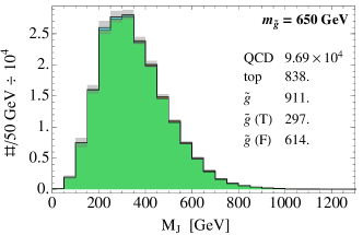
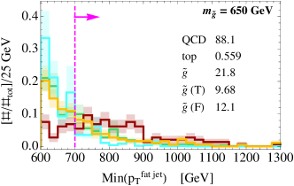
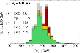
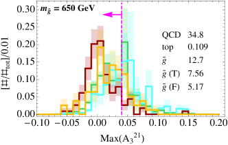
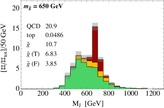
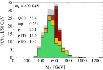
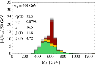
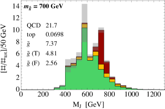
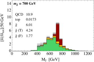
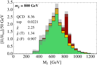
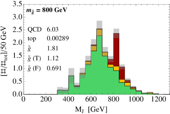
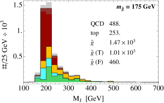
Fig. 7 illustrates the cut chain following the first fat-jet and cuts, for . As can be seen from the jet-mass distribution (a), the QCD background (green) completely dominates over both top background (cyan) and signal (split into ‘good’ signal in red, where the hardest two fat jets are within of the gluinos, and the rest in orange). Each unstacked histogram shows the unity-normalized distributions of a variable before cutting on it, for each signal and background component. The cut is indicated with a dashed magenta line, with events in the direction of the arrow kept for the next cut. (f) and (h) show the fat-jet-mass distribution before and after a conservative cut on axis contraction, shown in (g), is applied. (For a distribution of axis contraction at the same stage of cuts as (a), (b), see Fig. 4 (b)). The color cut loses very little signal but reduces background by almost one-half, and significantly improves the shape of the distribution, making the gluino peak stand out very clearly. This is also illustrated in Fig. 8 for a few other gluino masses. According to the MC comparison in Appendix B, the cuts on jet-substructure and color-flow observables in the heavy gluino analysis do not vary substantially among different generators, and the analysis is expected to be consistent within a small factor.
To estimate our analysis’ mass reach, we follow the maximum likelihood procedure for a shape analysis outlined in Cowan:2010js , but using the method CLsmethod . This involves using our predictions for the final jet-mass distributions, e.g. Fig. 8, to produce large collections of pseudodata for the ‘background-only’ and the ‘background + signal’ hypothesis, where the signal is scaled by some overall signal strength . (We ignore the statistical uncertainties of the MC prediction, as for such low event rates the Poisson fluctuations dominate.) By comparing the distributions of the test statistic computed for those pseudodata sets one can arrive at an expected signal strength exclusion, as well as the exclusion’s and fluctuations. The background normalization was allowed to float in each of these fits individually, making this a true shape analysis.
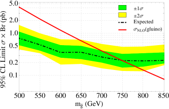
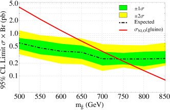
The resulting expected cross-section exclusions are compared to the gluino production cross section at LHC8 with in Fig. 9, both with and without the axis-contraction cut. The expected reach is and could be as high as 800 GeV, surprisingly high for a fully boosted search. With 5 of LHC8 data the reach is , higher than the LHC7 CMS search CMSrpvgluinobound5 and comparable to the ATLAS resolved search ATLASrpvgluinobound5 , which was a pure counting experiment. Since the boosted analysis has and is predominantly limited by statistics, more data should lead to better mass exclusion using the boosted analysis techniques discussed here.
Due to the small number of events surviving all the cuts, our estimate of the mass reach is not actually increased by the color-flow cuts, though the excluded cross section is increased for small , where more events survive all cuts. Furthermore, the color-flow cuts do decrease the background at little cost to the signal and may be useful to control systematic uncertainties on the background.
Exclusion could be improved by studying the fat-jet-mass distribution in control samples where no signal events are expected; a similar procedure was applied to the three-jet-mass distribution by CMS CMSrpvgluinobound36 ; CMSrpvgluinobound5 , effectively fixing the background normalization. This would increase our mass reach by , the small improvement being indicative that our simple shape analysis already does well in fixing the background normalization.
|
|
IV.4 Results for
While the recent ATLAS search for RPV gluinos excluded the mass range GeV ATLASrpvgluinobound5 , we still consider gluinos in this mass window as they provide a large sample of highly boosted signal events with which we can demonstrate the full discriminating power of our color-flow variables. Furthermore, we show that a dramatically higher signal purity than in ATLASrpvgluinobound5 can be achieved, which translates to a correspondingly higher cross section exclusion.
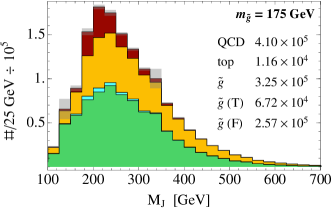
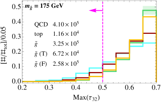
We find that the trigger requiring six jets with GeV yields the highest signal efficiency and tends to give boosted gluinos. Due to the abundance of signal we can cut hard on the substructure and color-flow variables. The cuts are outlined in Table 2 and illustrated in Fig. 10. While axis contraction was better suited for the soft cuts on color flow required by low signal numbers in the heavy gluino analysis, radial pull is more effective when we have enough signal to cut more aggressively. The result is an extremely powerful color-flow cut that keeps 12% of the combinatorially correct signal (of events surviving the previous cut step) but only 2% of combinatorially incorrect signal or background, and only 0.2% of Sherpa QCD background. The resulting mass distribution Fig. 10(g) is very signal-dominated and displays a clean resonance at 175 GeV 333We repeated this analysis for a 145 GeV gluino and found that the peak is indeed shifted appropriately to the left. This was to ensure that we are actually seeing a resonance, and not a falling jet-mass distribution shaped by the trigger and cuts.. Applying a -veto (assuming 70% tagging efficiency for quarks and a 1% light-jet mistag rate ATLASbtagger ) yields Fig. 10(h), with a resonance peak of gluino events and only about 1 background event in total. For other MC programs, as described in Appendix B, , which is smaller than Sherpa but still shows the discriminatory power of color-flow observables.
It is instructive to compare the radial-pull distribution after the kinematic substructure cuts Fig. 10(f) to Fig. 4 (left), which shows the same distribution before many of the kinematic and substructure cuts are applied. The similarity in the distributions (accounting for increased statistical uncertainty of the MC predictions after more cuts) suggests that radial pull is relatively uncorrelated with other substructure variables, and provides genuinely new discriminating power that cannot be accessed by simply making another cut more aggressive.
The counting experiment performed by ATLAS at LHC7 with 5 has excluded top-mass gluinos with . Treating our nearly background-free sample in a similar way would exclude at LHC8 with the same luminosity, decreasing to at 20 . Apart from excluding other possible RPV spectra, this can be relevant for different color representations decaying to three jets, which have different production cross sections. The shape analysis serves as a useful check on any discovered signal, since a resonance is clearly constructed. Furthermore, if a three-jet resonance in this mass range were to be found, one could use the alternative version of radial pull, Eq. (3), to distinguish a hadronized color-octet from some other state, as illustrated in Fig. 5.
V Conclusions
Jet-substructure variables are excellent tools in searches for boosted resonances. We have shown that such techniques can also be useful when applied to the boosted fraction of very heavy particles, such as RPV gluinos. Although this has recently been demonstrated in an LHC search for top-mass gluinos ATLASrpvgluinobound5 , we propose such search strategies also for heavier masses at LHC8. We use existing variables, such as -subjettiness, jet-mass symmetry, and subjet hierarchy, as well as our new color-flow variables, radial pull and axis contraction, to isolate a high-purity signal sample. Our suggested analysis strategy with aggressive cuts on these variables can be competitive with existing search strategies rouventhesis ; TEVATRONrpvgluinobound ; CMSrpvgluinobound36 ; CMSrpvgluinobound5 ; ATLASrpvgluinobound5 , while providing nearly independent systematic uncertainties. With 20 (5 ) at LHC8, it should be possible to probe boosted gluino-like resonances around the top mass with , corresponding to gluino branching fractions to three jets. Heavy gluinos can be excluded for GeV.
Additionally, we have shown that radial pull and axis contraction 444While working on this paper we learned that M. Freytsis, T. Volansky, and J. Walsh are independently exploring variables similar to axis shift, but in the context of boosted top tagging. Their results will appear shortly. appear to be powerful variables for distinguishing processes with different color flows, particularly for highly boosted events. We anticipate that they have applications in studies of other boosted colored objects, and may prove useful in distinguishing different models in the case that a boosted resonance is discovered.
Acknowledgements
We are grateful to T. Cohen, M. Freytsis, E. Izaguirre, and M. Lisanti for helpful discussions and comments on a draft version of this paper. We also thank M. Begel, E. Halkiadakis, J. Hobbs, D. Tsybychev, P. Meade, D. Miller, G. Salam, J. Shelton, G. Sterman, J. Thaler, and J. Wacker for helpful conversations. We especially thank P. Skands and T. Sjöstrand for their help with Pythia, and S. Höche and S. Schumann for their help with Sherpa. We also thank an anonymous referee for several useful suggestions. The work of D.C. was supported in part by the National Science Foundation under Grant PHY-0969739. RE is supported by the Department of Energy Early Career research program under Award Number DE-SC0008061. The work of B.S. was supported in part by the Harvard Center for the Fundamental Laws of Nature, the National Science Foundation under Grant PHY-0855591, and the Canadian Institute of Particle Physics. Research at the Perimeter Institute is supported in part by the Government of Canada through Industry Canada, and by the Province of Ontario through the Ministry of Research and Information (MRI). The work of D.C. and R.E. was conducted in part at the Aspen Center for Physics, supported by the National Science Foundation under Grant No. PHY-1066293. Some of the numerical calculations in this paper were performed on the Odyssey cluster supported by the FAS Research Group at Harvard University, as well as the facilities of the Shared Hierarchical Academic Research Computing Network (SHARCNET) and Compute/Calcul Canada.
Appendix A Review of RPV Gluinos
In addition to the superpotential terms of the Minimal Supersymmetric Standard Model, Standard Model gauge invariance allows terms that violate baryon () and lepton () number. and violation are strongly constrained by limits on proton decay and neutrino masses RPVreview . Often, -parity is imposed to remove these dangerous terms. However, if lepton number is conserved, the -violating RPV term
| (1) |
is allowed and only loosely constrained. Many theories accommodate RPV Ruderman:2012jd ; FileviezPerez:2009gr ; Goity:1994dq ; Chen:2010ss ; MFVsusy .
Models with can be challenging to observe, since the hadronic decay of supersymmetric particles suffer large QCD backgrounds. For RPV operators with one or more heavy-flavor quarks, multiple -tags, leptons, and missing energy can help distinguish the signal from backgrounds Brust:2012uf ; Allanach:2012vj ; Evans:2012bf . If the quarks are all light-flavored, however, no easy distinguishing property exists.
| Generator |
Preselection: 6 thin jets with and two fat jets with |
|
|
|
radial pull cut |
-veto |
|||||||||||||
| Gluino | Pythia 8 |
|
|
|
|
|
|
||||||||||||
| QCD | Sherpa |
|
|
|
|
|
|
||||||||||||
| POWHEG + Pythia 6 |
|
|
|
|
|
|
|||||||||||||
| POWHEG + Pythia 8 |
|
|
|
|
|
|
|||||||||||||
| Top | Sherpa |
|
|
|
|
|
|
||||||||||||
| Madgraph 5 + Pythia 6 |
|
|
|
|
|
|
|||||||||||||
| Madgraph 5 + Pythia 8 |
|
|
|
|
|
|
|||||||||||||
The couplings are subject to various constraints for different . The dominant constraint on comes from nucleon-antinucleon oscillation through an intermediate strange squark and gluino. The precise bound depends on the off-diagonal entries of the unknown left-right strange squark mixing matrix. If there is no mixing suppression, the bound is for TeV and TeV RPVreview . The bound is greatly relaxed if the mixing is suppressed.
The coupling induces strangeness-violating nucleon-antinucleon oscillation, leading to double nucleon decay processes such as and . Bounds extracted from this process are highly sensitive to hadronic and nuclear matrix elements, and range from to Goity:1994dq , with RPVreview quoting a value of for GeV.
The couplings and are even less constrained. Bounds can be imposed by requiring that the RPV couplings remain perturbative up to the GUT scale, giving .
We focus on models with light gluinos, which are pair-produced and each decay through an off-shell squark to three jets. Models exist in which the gauginos are naturally lighter than the scalars, including “split SUSY” ArkaniHamed:2004fb ; Giudice:2004tc ), leading to the possibility of a gluino LSP. The collider phenomenology depends on the gluino lifetime. Gluinos decaying through an off-shell squark and RPV couplings always hadronize before decaying, and depending on the magnitude of , may also give rise to displaced vertices. To see this, we estimate the gluino width in the limit :
| (2) |
Using a conservative value , then GeV with TeV and TeV, while GeV with the most relaxed bound . Since these are both well below , the gluino forms an -hadron prior to decay whenever , even when the RPV couplings are . We consider only prompt decays after hadronization; for long-lived and stopped gluinos, see e.g. Khachatryan:2010uf ; Graham:2012th .
Appendix B Monte Carlo Comparison
| (a) |
|
(b) |
|
| (a) |
|
(b) |
|
|||
| (c) |
|
(d) |
|
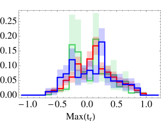
For the results presented in the main body of the paper, we have exclusively used Sherpa 1.4.0 to generate background event samples. Since our analysis includes a study of color-flow observables that may be sensitive to modeling of the parton shower and hadronization of colored objects, it is important to check how distributions of observables vary across Monte Carlo programs. Such a comparison also provides useful guidance for future substructure studies. We focus on QCD backgrounds, since these are dominant after all cuts, but also check distributions. We generated multijet backgrounds at parton-level with the Dijet package of POWHEG 1.0 Nason:2004rx ; Frixione:2007vw ; Alioli:2010xa , and the events were showered with the AUET2B tune ATLAS:2011gmi ; ATLAS:2011zja of Pythia 6.4.27 pythia6manual . POWHEG is an NLO generator, and the Dijet package generates 3-parton final states. We chose the combination of POWHEG + Pythia 6 because ATLAS found this provided a better detector-level description of the internal structure of high- jets than Pythia 6 alone ATLASrpvgluinobound5 . As a further check, we also showered the parton-level events with the default tune of Pythia 8.1.65 pythia8 . Matched top backgrounds were generated in Madgraph 5.1.5 Alwall:2011uj and showered in Pythia 6 and Pythia 8. Since the hadronization of gluinos and their subsequent RPV decay is only implemented in Pythia 8, we are unable to check the color-flow distributions of the signal against another MC program.
We compare distributions of the radial pull, axis contraction, , , and variables defined in the text at various stages of the cut chain. We use the cuts from our top-mass gluino analysis (Table 2), as some of these cuts were sensitive to the tails of certain observables such as radial pull. We summarize our results in Table 3, in which we show the cut efficiencies for QCD and top backgrounds generated by each MC program. In the table, we normalize the number of events after preliminary cuts to the Sherpa value, both because that event sample was normalized to data and to allow a direct comparison of each cut’s efficiency between MC generators. Furthermore, the fact that Sherpa generates matched samples with up to six partons suggests that it may give the best estimate of the number of events following the trigger and fat jet cuts.
Table 3 shows that, overall, the MC programs are consistent in their modeling of jet substructure, although the tails of the subjet hierarchy and radial pull distributions can differ somewhat between programs; the total efficiency after all cuts can vary by about a factor of 10 for QCD. In spite of the more pessimistic estimates from POWHEG + Pythia 6 and POWHEG + Pythia 8, however, there remains a gain in of from the radial pull cut, and for the mean number of events after all cuts for QCD. Furthermore, an optimization of the cut with the new MC program allows for some recovery of the gain in . For top backgrounds, the agreement is better, with a gain of for the radial pull cut, and with the number of events passing all cuts agreeing within a factor of 2-3. All MC generators studied thus show that radial pull, in conjunction with other jet substructure cuts, is extremely effective at isolating a pure signal sample for top-mass gluinos, although the degree of improvement differs between programs. Experimental study is needed to determine the precise gain anticipated from such cuts.
| (a) |
|
(b) |
|
We now provide details of the MC comparison for the QCD Background. The Dijet package of POWHEG is an NLO parton-level event generator. It generates dijet events at leading (Born) order, and then includes NLO corrections to generate three-parton events. Higher multiplicity jets are generated by the subsequent parton shower, making the efficiency of passing the six-jet trigger extremely low. The only cut that can be placed on QCD events is the of the dijet system prior to NLO emission (called the Born ) 555It is possible to generate weighted events in , but we find that the majority of events passing all cuts are those which marginally pass the six-jet trigger, and therefore generating many low-weight, high- events does not improve the statistics after all cuts are imposed.. This is in contrast with Sherpa, where six-parton final states could be generated directly with cuts on each parton. To choose the value of the POWHEG Born cut, we use the fact that parton emissions beyond LO are typically softer than the original hard scale; therefore, if applying a fat dijet cut of GeV to the showered sample (as in our top-mass gluino analysis), the corresponding cut on the Born should be similar but somewhat softer than this. 666 This can be understood physically. A configuration with two hard three-pronged fat jets would typically arise from a parton-level configuration with two partially-aligned partons recoiling off a third parton, with the shower providing additional hard subjets. In particular, most of one fat jet’s comes from a single hard parton, which has a momentum roughly bounded by the Born cut. We use the Born cut GeV, and we confirmed its validity by checking that the cross section passing trigger and fat jet cuts is the same for other generator-level cuts up to 140 GeV. With this cut, only 0.05% of MC events pass the preliminary six-jet trigger and fat jet cuts; even though we generated 500 million QCD events, we still suffer from small statistics for aggressive values of our substructure cuts, and only 1-2 such events pass the final radial pull cut from Section IV.4. The results for POWHEG+Pythia therefore have a much higher uncertainty than for Sherpa.
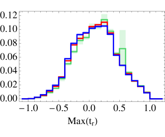
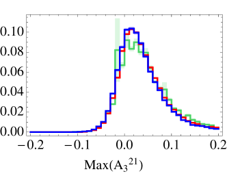
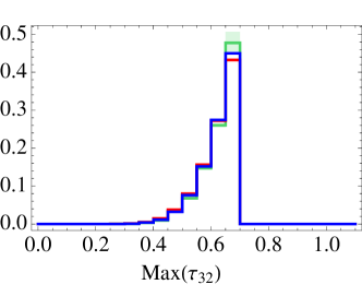
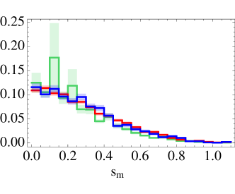
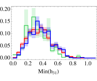
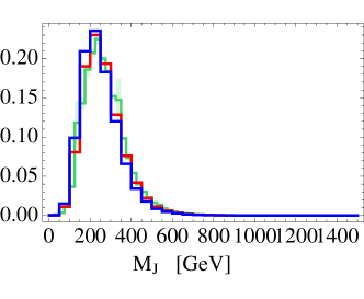
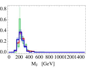
In Fig. 11, we compare the shapes of radial pull and axis contraction distributions for QCD samples generated with each MC program. The distributions are shown after the preliminary cuts of the top-mass gluino analysis (six-jet trigger and two fat jets GeV), and the shapes are similar for all generators. We also plot the distributions in Fig. 12 of each substructure variable before the cut on this variable as listed in Table 2. These distributions are largely consistent across different MC programs; the least-well-modeled variables are the subjet hierarchy and the radial pull , where we find that the cut efficiency of varies by at most a factor of two between MC descriptions, while the cuts on have efficiencies in the Pythia samples that are approximately six times higher than the Sherpa prediction. Some of this variation, especially for the cut, may be due to Sherpa generating up to 6 jets at the matrix-element level while POWHEG must rely on the shower. This suggests that Sherpa’s predictions might be more trustworthy. At any rate, the statistical uncertainties are very large because only one or two MC events pass cuts from the Pythia samples. For completeness, we also plot the fat-jet mass distributions before and after jet substructure cuts in Fig. 13,
Figs. 11-12 therefore demonstrate that our substructure analysis is generally robust across different MC event generators for QCD backgrounds. The most sensitive observables are the tails of the radial pull and axis contraction variables, which can change background cut efficiencies by up to a factor of , but is so large that the results are not invalidated. Together with the already outlined comparison of top backgrounds, which are anyway subdominant to QCD after a -veto, this provides evidence that the Sherpa analysis is reliable.
References
- (1) [ATLAS Collaboration], ATLAS-CONF-2012-109.
- (2) S. Chatrchyan et al. [CMS Collaboration], arXiv:1207.1898 [hep-ex].
- (3) [ATLAS Collaboration], ATLAS-CONF-2012-103.
- (4) [CMS Collaboration], CMS PAS SUS-11-006.
- (5) G. Aad et al. [ATLAS Collaboration], arXiv:1208.2590 [hep-ex].
- (6) [CMS Collaboration], CMS PAS SUS-11-022.
- (7) S. Chatrchyan et al. [CMS Collaboration], arXiv:1205.3933 [hep-ex].
- (8) G. Aad et al. [ATLAS Collaboration], Phys. Rev. Lett. 108, 181802 (2012) [arXiv:1112.3832 [hep-ex]].
- (9) G. Aad et al. [ATLAS Collaboration], arXiv:1208.4688 [hep-ex].
- (10) G. F. Sterman and S. Weinberg, “Jets from Quantum Chromodynamics,” Phys. Rev. Lett. 39 (1977) 1436.
- (11) R. S. Chivukula, M. Golden and E. H. Simmons, “Six Jet Signals of Highly Colored Fermions,” Phys. Lett. B 257 (1991) 403.
- (12) R. S. Chivukula, M. Golden and E. H. Simmons, “Multi - Jet Physics at Hadron Colliders,” Nucl. Phys. B 363 (1991) 83.
- (13) E. Farhi and L. Susskind, “A Technicolored G.U.T.,” Phys. Rev. D 20 (1979) 3404.
- (14) W. J. Marciano, Phys. Rev. D 21 (1980) 2425.
- (15) P. H. Frampton and S. L. Glashow, Phys. Rev. Lett. 58 (1987) 2168.
- (16) P. H. Frampton and S. L. Glashow, Phys. Lett. B 190 (1987) 157.
- (17) Based on work by S-H. Chuang, R. Essig, E. Halkiadakis, A. Lath, S.Thomas; see Ch. 6 in R. Essig, AAT-3349692, PhD Thesis, Rutgers University, 2008, http://hdl.rutgers.edu/1782.2/rucore10001600001.ETD.17462.
- (18) L. J. Hall and M. Suzuki, Nucl. Phys. B 231, 419 (1984).
- (19) R. Barbier et al., Phys. Rept. 420, 1 (2005) [hep-ph/0406039].
- (20) J. Alwall, M. -P. Le, M. Lisanti and J. G. Wacker, Phys. Lett. B 666, 34 (2008) [arXiv:0803.0019 [hep-ph]].
- (21) C. Kilic, T. Okui and R. Sundrum, JHEP 0807 (2008) 038 [arXiv:0802.2568 [hep-ph]].
- (22) C. Kilic and T. Okui, JHEP 1004 (2010) 128 [arXiv:1001.4526 [hep-ph]].
- (23) D. Alves et al. [LHC New Physics Working Group Collaboration], J. Phys. G 39 (2012) 105005 [arXiv:1105.2838 [hep-ph]].
- (24) G. Marques Tavares and M. Schmaltz, Phys. Rev. D 84 (2011) 054008 [arXiv:1107.0978 [hep-ph]].
- (25) C. Gross, G. M. Tavares, C. Spethmann and M. Schmaltz, arXiv:1209.6375 [hep-ph].
- (26) A. Hook, E. Izaguirre, M. Lisanti and J. G. Wacker, Phys. Rev. D 85, 055029 (2012) [arXiv:1202.0558 [hep-ph]].
- (27) M. Asano, K. Rolbiecki and K. Sakurai, arXiv:1209.5778 [hep-ph].
- (28) D. E. Kaplan and M. D. Schwartz, Phys. Rev. Lett. 101, 022002 (2008) [arXiv:0804.2477 [hep-ph]].
- (29) T. Aaltonen et al. [CDF Collaboration], Phys. Rev. Lett. 107, 042001 (2011) [arXiv:1105.2815 [hep-ex]].
- (30) S. Chatrchyan et al. [CMS Collaboration], Phys. Rev. Lett. 107, 101801 (2011) [arXiv:1107.3084 [hep-ex]].
- (31) S. Chatrchyan et al. [CMS Collaboration], arXiv:1208.2931 [hep-ex].
- (32) G. Aad et al. [ATLAS Collaboration], arXiv:1210.4813 [hep-ex].
- (33) B. C. Allanach and B. Gripaios, JHEP 1205, 062 (2012) [arXiv:1202.6616 [hep-ph]].
- (34) C. Brust, A. Katz, S. Lawrence and R. Sundrum, JHEP 1203, 103 (2012) [arXiv:1110.6670 [hep-ph]].
- (35) C. Brust, A. Katz and R. Sundrum, JHEP 1208, 059 (2012) [arXiv:1206.2353 [hep-ph]].
- (36) J. A. Evans and Y. Kats, arXiv:1209.0764 [hep-ph].
- (37) J. Thaler and K. Van Tilburg, JHEP 1103, 015 (2011) [arXiv:1011.2268 [hep-ph]].
- (38) I. W. Stewart, F. J. Tackmann and W. J. Waalewijn, Phys. Rev. Lett. 105 (2010) 092002 [arXiv:1004.2489 [hep-ph]].
- (39) J. Thaler and K. Van Tilburg, JHEP 1202, 093 (2012) [arXiv:1108.2701 [hep-ph]].
- (40) J. Gallicchio and M. D. Schwartz, Phys. Rev. Lett. 105, 022001 (2010) [arXiv:1001.5027 [hep-ph]].
- (41) A. Bassetto, M. Ciafaloni and G. Marchesini, Phys. Rept. 100, 201 (1983).
- (42) A. Hook, M. Jankowiak and J. G. Wacker, JHEP 1204, 007 (2012) [arXiv:1102.1012 [hep-ph]].
- (43) J. Gallicchio, J. Huth, M. Kagan, M. D. Schwartz, K. Black and B. Tweedie, JHEP 1104, 069 (2011) [arXiv:1010.3698 [hep-ph]].
- (44) Y. Cui, Z. Han and M. D. Schwartz, Phys. Rev. D 83, 074023 (2011) [arXiv:1012.2077 [hep-ph]].
- (45) J. Gallicchio and M. D. Schwartz, Phys. Rev. Lett. 107, 172001 (2011) [arXiv:1106.3076 [hep-ph]].
- (46) L. G. Almeida, S. J. Lee, G. Perez, I. Sung and J. Virzi, Phys. Rev. D 79, 074012 (2009) [arXiv:0810.0934 [hep-ph]].
- (47) J. M. Butterworth, A. R. Davison, M. Rubin and G. P. Salam, Phys. Rev. Lett. 100, 242001 (2008) [arXiv:0802.2470 [hep-ph]].
- (48) S. D. Ellis, C. K. Vermilion and J. R. Walsh, Phys. Rev. D 80, 051501 (2009) [arXiv:0903.5081 [hep-ph]].
- (49) T. Plehn, G. P. Salam and M. Spannowsky, Phys. Rev. Lett. 104, 111801 (2010) [arXiv:0910.5472 [hep-ph]].
- (50) D. Krohn, J. Thaler and L. -T. Wang, JHEP 1002, 084 (2010) [arXiv:0912.1342 [hep-ph]].
- (51) G. D. Kribs, A. Martin, T. S. Roy and M. Spannowsky, Phys. Rev. D 81, 111501 (2010) [arXiv:0912.4731 [hep-ph]].
- (52) G. Brooijmans, ATL-PHYS-CONF-2008-008.
- (53) D. E. Soper and M. Spannowsky, Phys. Rev. D 84, 074002 (2011) [arXiv:1102.3480 [hep-ph]].
- (54) J. M. Butterworth, J. R. Ellis and A. R. Raklev, JHEP 0705, 033 (2007) [hep-ph/0702150 [hep-ph]].
- (55) L. G. Almeida, S. J. Lee, G. Perez, G. Sterman and I. Sung, Phys. Rev. D 82, 054034 (2010) [arXiv:1006.2035 [hep-ph]].
- (56) M. Jankowiak and A. J. Larkoski, JHEP 1106, 057 (2011) [arXiv:1104.1646 [hep-ph]].
- (57) S. D. Ellis, A. Hornig, T. S. Roy, D. Krohn and M. D. Schwartz, Phys. Rev. Lett. 108, 182003 (2012) [arXiv:1201.1914 [hep-ph]].
- (58) J. M. Butterworth, B. E. Cox and J. R. Forshaw, Phys. Rev. D 65, 096014 (2002) [hep-ph/0201098].
- (59) M. Jankowiak and A. J. Larkoski, JHEP 1204, 039 (2012) [arXiv:1201.2688 [hep-ph]].
- (60) G. P. Salam, Eur. Phys. J. C 67, 637 (2010) [arXiv:0906.1833 [hep-ph]].
- (61) J. Thaler and L. -T. Wang, JHEP 0807, 092 (2008) [arXiv:0806.0023 [hep-ph]].
- (62) D. E. Kaplan, K. Rehermann, M. D. Schwartz and B. Tweedie, Phys. Rev. Lett. 101, 142001 (2008) [arXiv:0806.0848 [hep-ph]].
- (63) V. M. Abazov et al. [D0 Collaboration], Phys. Rev. D 83, 092002 (2011) [arXiv:1101.0648 [hep-ex]].
- (64) G. Aad et al. [ATLAS Collaboration], JHEP 1205, 128 (2012) [arXiv:1203.4606 [hep-ex]].
- (65) G. Aad et al. [Atlas Collaboration], Phys. Rev. D 83, 052003 (2011) [arXiv:1101.0070 [hep-ex]].
- (66) G. Aad et al. [ATLAS Collaboration], arXiv:1206.5369 [hep-ex].
- (67) [CMS Collaboration], CMS-PAS-JME-10-013.
- (68) T. Aaltonen et al. [CDF Collaboration], Phys. Rev. D 85, 091101 (2012) [arXiv:1106.5952 [hep-ex]].
- (69) [ATLAS Collaboration], ATLAS-CONF-2011-073.
- (70) S. Chatrchyan et al. [CMS Collaboration], JHEP 1206, 160 (2012) [arXiv:1204.3170 [hep-ex]].
- (71) M. H. Seymour, Z. Phys. C 62, 127 (1994).
- (72) A. Abdesselam et al., Eur. Phys. J. C 71, 1661 (2011) [arXiv:1012.5412 [hep-ph]].
- (73) T. Plehn and M. Spannowsky, J. Phys. G G 39, 083001 (2012) [arXiv:1112.4441 [hep-ph]].
- (74) A. Altheimer et al., J. Phys. G G 39, 063001 (2012) [arXiv:1201.0008 [hep-ph]].
- (75) G. Brooijmans et al. [New Physics Working Group Collaboration], arXiv:1005.1229 [hep-ph]; A. R. Raklev, G. P. Salam and J. G. Wacker, SLAC-REPRINT-2012-045.
- (76) D. Curtin, R. Essig, B. Shuve, In preparation.
- (77) J. M. Butterworth, J. R. Ellis, A. R. Raklev and G. P. Salam, Phys. Rev. Lett. 103, 241803 (2009) [arXiv:0906.0728 [hep-ph]].
- (78) J. D. Bjorken, Int. J. Mod. Phys. A 7, 4189 (1992).
- (79) J. D. Bjorken, Phys. Rev. D 47, 101 (1993).
- (80) R. S. Fletcher and T. Stelzer, Phys. Rev. D 48, 5162 (1993) [hep-ph/9306253].
- (81) V. D. Barger, R. J. N. Phillips and D. Zeppenfeld, Phys. Lett. B 346, 106 (1995) [hep-ph/9412276].
- (82) M. Fairbairn, A. C. Kraan, D. A. Milstead, T. Sjostrand, P. Z. Skands and T. Sloan, Phys. Rept. 438, 1 (2007) [hep-ph/0611040].
- (83) C. F. Berger, T. Kucs and G. F. Sterman, Phys. Rev. D 68, 014012 (2003) [hep-ph/0303051].
- (84) T. Sjostrand, S. Mrenna and P. Z. Skands, JHEP 0605, 026 (2006) [hep-ph/0603175].
- (85) N. Desai and P. Z. Skands, arXiv:1109.5852 [hep-ph].
- (86) T. Sjostrand and P. Z. Skands, Nucl. Phys. B 659, 243 (2003) [hep-ph/0212264].
- (87) T. Sjostrand, S. Mrenna and P. Z. Skands, Comput. Phys. Commun. 178, 852 (2008) [arXiv:0710.3820 [hep-ph]].
- (88) W. Beenakker, R. Hopker and M. Spira, hep-ph/9611232; W. Beenakker, M. Klasen, M. Kramer, T. Plehn, M. Spira and P. M. Zerwas, Phys. Rev. Lett. 83, 3780 (1999) [Erratum-ibid. 100, 029901 (2008)] [hep-ph/9906298].
- (89) T. Gleisberg, S. .Hoeche, F. Krauss, M. Schonherr, S. Schumann, F. Siegert and J. Winter, JHEP 0902, 007 (2009) [arXiv:0811.4622 [hep-ph]].
- (90) F. Krauss, R. Kuhn and G. Soff, JHEP 0202, 044 (2002) [hep-ph/0109036]; S. Schumann and F. Krauss, JHEP 0803, 038 (2008) [arXiv:0709.1027 [hep-ph]]; T. Gleisberg and S. Hoeche, JHEP 0812, 039 (2008) [arXiv:0808.3674 [hep-ph]]; S. Hoeche, F. Krauss, S. Schumann and F. Siegert, JHEP 0905, 053 (2009) [arXiv:0903.1219 [hep-ph]].
- (91) M. Begel and D. Tsybychev, private communication.
- (92) M. Cacciari and G. P. Salam, Phys. Lett. B 641, 57 (2006) [hep-ph/0512210]; M. Cacciari, G. P. Salam and G. Soyez, Eur. Phys. J. C 72, 1896 (2012) [arXiv:1111.6097 [hep-ph]].
- (93) M. Cacciari, G. P. Salam and G. Soyez, JHEP 0804, 063 (2008) [arXiv:0802.1189 [hep-ph]].
- (94) A. Falkowski, D. Krohn, L. -T. Wang, J. Shelton and A. Thalapillil, Phys. Rev. D 84, 074022 (2011) [arXiv:1006.1650 [hep-ph]].
- (95) L. G. Almeida, S. J. Lee, G. Perez, G. F. Sterman, I. Sung and J. Virzi, Phys. Rev. D 79, 074017 (2009) [arXiv:0807.0234 [hep-ph]].
- (96) S. D. Ellis, C. K. Vermilion and J. R. Walsh, Phys. Rev. D 81, 094023 (2010) [arXiv:0912.0033 [hep-ph]].
- (97) G. Soyez, “Pile-up subtraction for jet , masses, and shapes”, BOOST 2012 talk.
- (98) A. L. Read, J. Phys. G 28 (2002) 2693, doi:10.1088/0954-3899/28/10/313.
- (99) G. Cowan, K. Cranmer, E. Gross and O. Vitells, Eur. Phys. J. C 71, 1554 (2011) [arXiv:1007.1727 [physics.data-an]].
- (100) The ATLAS Collaboration, ATLAS-CONF-2011-102, July 2011.
- (101) J. T. Ruderman, T. R. Slatyer and N. Weiner, arXiv:1207.5787 [hep-ph].
- (102) P. Fileviez Perez and S. Spinner, Phys. Rev. D 80, 015004 (2009) [arXiv:0904.2213 [hep-ph]].
- (103) J. L. Goity and M. Sher, Phys. Lett. B 346, 69 (1995) [Erratum-ibid. B 385, 500 (1996)] [hep-ph/9412208].
- (104) S. -L. Chen, D. K. Ghosh, R. N. Mohapatra and Y. Zhang, JHEP 1102, 036 (2011) [arXiv:1011.2214 [hep-ph]].
- (105) C. Csaki, Y. Grossman and B. Heidenreich, Phys. Rev. D 85, 095009 (2012) [arXiv:1111.1239 [hep-ph]].
- (106) N. Arkani-Hamed and S. Dimopoulos, JHEP 0506, 073 (2005) [hep-th/0405159].
- (107) G. F. Giudice and A. Romanino, Nucl. Phys. B 699, 65 (2004) [Erratum-ibid. B 706, 65 (2005)] [hep-ph/0406088].
- (108) V. Khachatryan et al. [CMS Collaboration], Phys. Rev. Lett. 106, 011801 (2011) [arXiv:1011.5861 [hep-ex]].
- (109) P. W. Graham, D. E. Kaplan, S. Rajendran and P. Saraswat, JHEP 1207, 149 (2012) [arXiv:1204.6038 [hep-ph]].
- (110) P. Nason, JHEP 0411, 040 (2004) [hep-ph/0409146].
- (111) S. Frixione, P. Nason and C. Oleari, JHEP 0711, 070 (2007) [arXiv:0709.2092 [hep-ph]].
- (112) S. Alioli, K. Hamilton, P. Nason, C. Oleari and E. Re, JHEP 1104, 081 (2011) [arXiv:1012.3380 [hep-ph]].
- (113) [ATLAS Collaboration], ATL-PHYS-PUB-2011-008.
- (114) [ATLAS Collaboration], ATL-PHYS-PUB-2011-009.
- (115) J. Alwall, M. Herquet, F. Maltoni, O. Mattelaer and T. Stelzer, JHEP 1106, 128 (2011) [arXiv:1106.0522 [hep-ph]].
