Modeling with Copulas and Vines in
Estimation of Distribution Algorithms

Abstract

The aim of this work is studying the use of copulas and vines in the optimization with Estimation of Distribution Algorithms (EDAs). Two EDAs are built around the multivariate product and normal copulas, and other two are based on pair-copula decomposition of vine models. Empirically we study the effect of both marginal distributions and dependence structure separately, and show that both aspects play a crucial role in the success of the optimization. The results show that the use of copulas and vines opens new opportunities to a more appropriate modeling of search distributions in EDAs.

1 Introduction

Estimation of distribution algorithms (EDAs) [31, 33] are stochastic optimization methods characterized by the explicit use of probabilistic models. EDAs explore the search space by sampling a probability distribution (search distribution) previously built from promising solutions.

Most existing continuous EDAs are based on either the multivariate normal distribution or models derived from it [9, 28]. However, in situations where empirical evidence reveals significant departures from the normality assumption, these EDAs construct incorrect models of the search space. A solution come with the copula function [34], which provides a way to separate the statistical properties of each variable from the dependence structure: first, the marginal distributions are fitted using a rich variety of univariate models available, and then, the dependence between the variables is modeled using a copula. However, the multivariate copula approach has limitations. The number of multivariate copulas is rather limited, and usually these copulas have only one parameter to describe the overall dependence. Thus, this approach is not appropriate when all the pairs of variables do not have the same type or strength of dependence. For instance, the $t$-copula uses one correlation coefficient per each pair of variables, but has only a single degree of freedom parameter to characterize the tail dependence for all pairs.

An alternative approach to this problem is the pair-copula construction method (PCC) [6, 7, 26], which allows to built multivariate distributions using only bivariate copulas. PCC models of multivariate distributions are represented in a graphical way as a sequence of nested trees, which are called vines. These graphical models provide a powerful and flexible tool to deal with complex dependences as far as the pair-copulas in the decomposition can be of different copula families.

In recent years, several copula-based EDAs have been proposed in the literature. The authors have studied the behavior of these algorithms in test functions [12, 17, 39, 45, 48, 44, 21, 22] and a real-world problem [46]. Indeed, the use of copulas has been identified as one of the emerging trends in the optimization of real-valued problems using EDAs [25]. In this work, various models based on copula theory are combined in an EDA: two models are built using the multivariate product and normal copulas and other two are based on two PCC models called C-vine and D-vine. We empirically evaluate the performance of these algorithms on a set of test functions and show that vine-based EDAs are better endowed to deal with problems with different dependences between pair of variables.

The paper is organized as follows. Section 2 introduces the notion of copula and describes two EDAs based on the multivariate product and normal copulas, respectively. Section 3 presents the notion and terminology of vines and introduces two EDAs based on C-vine and D-vine models, respectively. Section 4 reports and discuses the empirical investigation. Finally, Section 5 gives the conclusions.

2 Two Continuous EDAs Based on Multivariate Copulas

We start with some definitions from copula theory [27, 34]. Consider $n$ random variables $\mathbf{X}=\left(X_{1},\ldots,X_{n}\right)$ with joint cumulative distribution function $F$ and joint density function $f$. Let $\mathbf{x}=\left(x_{1},\ldots,x_{n}\right)$ be an observation of $\mathbf{X}$. A copula $C$ is a multivariate distribution with uniformly distributed marginals $U\left(0,1\right)$ on $\left[0,1\right]$. Sklar’s theorem [43] states that every multivariate distribution $F$ with marginals $F_{1},F_{2},\ldots,F_{n}$ can be written as

$$F\left(x_{1},\ldots,x_{n}\right)=C\left(F\left(x_{1}\right),\ldots,F\left(x_{n}\right)\right)$$

and

$$C\left(u_{1},\ldots,u_{n}\right)=F\left(F_{1}^{(-1)}\left(u_{1}\right),\ldots,F_{n}^{(-1)}\left(u_{n}\right)\right)$$

where $F_{i}^{(-1)}$ are the inverse distribution functions of the marginals. If $F$ is continuous then $C\left(u_{1},\ldots,u_{n}\right)$ is unique. The notion of copulas separates the effect of dependence and margins in a joint distribution [29]. The copula $C$ provides all information about the dependence structure of $F$, independently of the specification of the marginal distributions.

An immediate consequence of Sklar’s theorem is that random variables are independent if and only if their underlying copula is the independence or product copula $C_{\textrm{I}}$, which is given by

$$C_{\textrm{I}}\left(u_{1},\ldots,u_{n}\right)=u_{1}.\ldots.u_{n}.$$ (1)

The UMDA proposed in [31] assumes a model of independence of normal margins. Therefore, an EDA based on the product copula is a generalization of the UMDA, which also supports other types of marginal distributions.

Besides UMDA, in [31] the authors also proposed an EDA based on the multivariate normal distribution. They called it Estimation of the Multivariate Normal Algorithm (EMNA). It turns out that, indeed EMNA can be also reformulated in copula terms: a normal copula plus normal margins.

The Gaussian Copula Estimation of Distribution Algorithm (GCEDA) proposed in [45, 3] uses the multivariate normal (or Gaussian) copula, which is given by

$$C_{\textrm{N}}\left(u_{1},\ldots,u_{n};R\right)=\Phi_{R}\left(\Phi^{-1}\left(u_{1}\right),\ldots,\Phi^{-1}\left(u_{n}\right)\right),$$ (2)

where $\Phi_{R}$ is the standard multivariate normal distribution with correlation matrix $R$, and $\Phi^{-1}$ denotes the inverse of the standard univariate normal distribution. This copula allows the construction of multivariate distributions with non-normal margins. If this is the case, the joint density is no longer the multivariate normal, though the normal dependence structure is preserved. Therefore, with normal margins, GCEDA is equal to EMNA, otherwise they are different.

If the marginal distributions are non-normal, the correlation matrix is estimated using the inversion of the non-parametric estimator Kendall’s tau $\hat{R}_{ij}=\sin\left(\nicefrac{{\pi}}{{2}}\hat{\tau}_{ij}\right)$ for each pair of variables $i,j=1,\ldots,n$ [34]. If the resulting matrix $\hat{R}$ is not positive-definite, the correction proposed in [38] can be applied.

In this work, all margins used by the algorithms are always of the same type, either normal (Gaussian) or empirical smoothed with a normal kernel. In particular, the estimation of the normal margin $\hat{F_{i}}\backsim\mathcal{N}\left(x_{i};\hat{\mu}_{i},\hat{\sigma}_{i}^{2}\right)$ requires the computation of the mean $\hat{\mu_{i}}$ and variance $\hat{\sigma_{i}}^{2}$ from the selected population. The empirical margin is estimated using the normal kernel estimator given by

$$\hat{F}_{i}\left(t\right)=\frac{1}{N}\sum_{j=1}^{N}\Phi\left(\frac{t-y_{j}}{h}\right),$$

where the set $\left\{y_{1},\ldots,y_{N}\right\}$ is the sample of the $i^{th}$ variable of $\mathbf{X}$ in the selected population with $N$ individuals. The bandwidth parameter $h$ is computed according to the rule-of-thumb of [42]. In this paper, the subscripts g and e in the name of the algorithms denote the use of Gaussian and empirical margins, respectively (e.g., UMDA${}_{\textrm{g}}$ and GCEDA${}_{\textrm{e}}$).

The generation of a new individual in GCEDA${}_{\textrm{g}}$ and GCEDA${}_{\textrm{e}}$ starts with the simulation of a vector $\left(u_{1},\ldots,u_{n}\right)$ from the multivariate normal copula [16]. In GCEDA${}_{\textrm{g}}$, the inverse distribution function $x_{i}=\hat{F}_{i}^{-1}\left(u_{i};\hat{\mu}_{i},\hat{\sigma}_{i}^{2}\right)$ is used to obtain each $x_{i}$ of the new individual. In GCEDA${}_{\textrm{e}}$, $x_{i}$ is found by solving the inverse of the marginal cumulative distribution using the Newton-Raphson method [4].

3 EDAs Based on Vines

This section provides a brief description of the C-vine and D-vine models and the motivation for using them to construct the search distributions in EDAs. We also introduce CVEDA and DVEDA, our third and fourth algorithms.

3.1 From Multivariate Copulas to Vines

The multivariate copula approach has several limitations. Most of the available parametric copulas are bivariate and the multivariate extensions usually describe the overall dependence by means of only one parameter. This approach is not appropriate when there are pairs of variables with different type or strength of dependence. The pair-copula construction method (PCC) is an alternative approach to this problem. PCC method was originally proposed in [26] and this result was later developed in [6, 7, 26]. The decomposition of a multivariate distribution in pair-copulas is a general and flexible method for constructing multivariate distributions. In PCC models, bivariate copulas are used as building blocks. The graphical representation of these constructions involves a sequence of nested trees, called regular vines. Pair-copula constructions of regular vines allows to model a rich variety of types of dependences as far as the bivariate copulas can belong to different families.

3.2 Pair-Copula Constructions of C-vines and D-vines

Vines are dependence models of a multivariate distribution function based on a decomposition of $f\left(x_{1},\ldots,x_{n}\right)$ into bivariate copulas and marginal densities. A vine on $n$ variables is a nested set of trees $T_{1},\ldots,T_{n-1}$, where the edges of tree $j$ are the nodes of the tree $j+1$ with $j=1,\ldots,n-2$. Regular vines constitute a special case of vines in which two edges in tree $j$ are joined by an edge in tree $j+1$ only if these edges share a common node.

Two instances of regular vines are the canonical (C) and drawable (D) vines. In Figure 1, a graphical representation of a C-vine and D-vine for four dimensions is given. Each graphical model gives a specific way of decomposing the density. In particular, for a C-vine, $f\left(x_{1},\ldots,x_{n}\right)$ is given by

$$\prod_{k=1}^{n}f\left(x_{k}\right)\prod_{j=1}^{n-1}\prod_{i=1}^{n-j}c_{j,,j+i|i,\ldots,,j-1}\left(F\left(x_{j}|x_{1},\ldots,x_{j\text{-}1}\right),F\left(x_{j+i}|x_{1},\ldots,x_{j-1}\right)\right),$$ (3)

and for a D-vine, the density is equal to

$$\prod_{k=1}^{n}f\left(x_{k}\right)\prod_{j=1}^{n-1}\prod_{i=1}^{n-j}c_{i,i+j|i+1,\ldots,i+j-1}\left(F\left(x_{i}|x_{i+1},\ldots,x_{i+j-1}\right),F\left(x_{i+j}|x_{i+1},\ldots,x_{i+j\text{-}1}\right)\right),$$ (4)

where $j$ identifies the trees and $i$ denotes the edges in each tree.

(a)

(b)

Figure 1: Four-dimensional C-vine (a) and D-vine (b). In a C-vine, each tree $T_{j}$ has a unique node with $n-j$ edges. The node with $n-1$ edges in tree is called the root. In a D-vine, no node is connected to more than two edges.

Note that in (3) and (4) the joint density consists of marginal densities $f\left(x_{k}\right)$ and pair-copula densities evaluated at conditional distribution functions of the form $F\left(x\mid\mathbf{v}\right)$.

In [26] it is showed that conditional distribution of pair-copulas constructions are given by

$$F\left(x\mid\mathbf{v}\right)=\frac{\partial C_{xv_{j}\mid\mathbf{v}_{-j}}\left(F\left(x\mid\mathbf{v}_{-j}\right),F\left(v_{j}\mid\mathbf{v}_{-j}\right)\right)}{\partial F\left(v_{j}\mid\mathbf{v}_{-j}\right)},$$ (5)

where $C_{xv_{j}\mid\mathbf{v}_{-j}}$ is a bivariate copula distribution function, $\mathbf{v}$ is a $n$-dimensional vector, $v_{j}$ is the $j$ components of $\mathbf{v}$ and $\mathbf{v}_{-j}$ denotes the remaining component. The recursive evaluation of $F\left(x\mid\mathbf{v}\right)$ yields the expression

$$F\left(x\mid v\right)=\frac{\partial C_{xv}\left(F_{x}\left(x\right),F_{v}\left(v\right)\right)}{\partial F_{v}\left(v\right)}.$$

For the special case (unconditional) when $v$ is univariate, and $x$ and $v$ are standard uniform, $F\left(x\mid v\right)$ reduces further to

$$F\left(x\mid v\right)=\frac{\partial C_{xv}\left(x,v,\Theta\right)}{\partial v}.$$

where $\mathbf{\Theta}$ is the set of parameters for the bivariate copula of the joint distribution function of $x$ and $v$. To facilitate de computation of $F\left(x\mid v\right)$, the function

$$h\left(x,v;\theta\right)=F\left(x\mid v\right)=\frac{\partial C_{xv}\left(x,v;\Theta\right)}{\partial v},$$ (6)

is defined. The inverse of $h$ with respect to the first variable $h^{-1}$ is also defined. The expressions of these functions of the bivariate copulas used in this work are given in Appendix A.

3.3 Vine Estimation of Distribution Algorithms

Vine Estimation of Distribution Algorithms (VEDAs) [21, 44] are a class of EDAs that uses vines to model the search distributions. CVEDA and DVEDA are VEDAs based on C-vines and D-vines, respectively. Now we describe the particularities of the estimation and simulation steps of these algorithms.

3.3.1 Estimation

The estimation procedures of C-vines and D-vines proposed and developed in [1] consist of the following main steps: selection of a specific factorization, choice of the pair-copula types in the factorization, and estimation of the copula parameters. Next we describe these steps according to our implementation.

1. Selection of a specific factorization:

   The selection of a specific pair-copula decomposition implies to choose an appropriate order of the variables, which can be obtained by several ways: given as parameter, selected at random, chosen by greedy heuristics. We use greedy heuristics for detecting the most important bivariate dependences.

   Assumed a specific factorization, the first step of the estimation procedure consist in assigning weights to the edges. As weight we use the absolute value of the empirical Kendall’s tau between pair of variables [34]. The next step consist in determining the appropriate order of the variables of the decomposition, which depend on the type of pair-copula decomposition:

   • In a C-vine, the tree that maximizes the sum of the weights of one node (the root) to the others is chosen by the greedy heuristic as the appropriate factorization.

   • In a D-vine, the first tree is that which maximizes the weighted sequence of the original variables. In [10], this problem is transformed into a traveling salesman problem (TSP) instance by adding a dummy node with weight zero on all edges to the other nodes. For efficiency, we use the cheapest insertion heuristic, an approximate solution of TSP presented in [37]. In a D-vine, the structure of remaining trees is completely determined by the structure of the first.

   A pair-copula decomposition has $n-1$ trees and requires to fit $\nicefrac{{n\left(n-1\right)}}{{2}}$ copulas. Assuming conditional independence might simplify the estimation step, since if $X$ and $Y$ are conditionally independent given $\mathbf{V}$, then $c_{xy\mid\mathbf{v}}\left(F_{x\mid\mathbf{v}}\left(x\mid\mathbf{v}\right),\,F_{y\mid\mathbf{v}}\left(y\mid\mathbf{v}\right)\right)=1$. This property is used by a model selection procedure proposed in [10], which consists in truncating the pair-copula decomposition at specific tree level, fitting the product copula in the subsequent trees. For detecting the truncation tree level, this procedure uses either the Akaike Information Criterion (AIC) [2] or the Bayesian Information Criterion (BIC) [41], such that the tree $T_{j+1}$ is expanded if the value of the information criteria calculated up to the tree $T_{j+1}$ is smaller than the value obtained up to the previous tree. Otherwise, the vine is truncated at tree level $T_{j}$.

2. Choice of the pair-copula types in the factorization and estimation of the copula parameters.

   1. Determine which pair-copula types to use in tree 1 using the original data by applying a goodness of fit test.

   2. Compute observations (i.e. conditional distribution functions) using the copula parameters from tree 1 and the $h\left(.\right)$ function.

   3. Determine the pair-copula types to use in tree 2 in the same way as in tree 1 using the observations from (b).

   4. Repeat (b) and (c) for the following trees.

   Selection of pair-copulas is accomplished in different ways [20]. In this work, the Cramér-von Mises statistics

   $$S_{N}=\sum_{i=1}^{N}\left(C_{\textrm{$\mbox{E}$}}(u_{i,}v_{i})-C_{\mathbf{\Theta}}(u_{i},v_{i})\right)^{2}$$ (7)

   is minimized. $N$ is the sample size, $\mathbf{\Theta}$ is the set of parameters of a bivariate copula $C_{\mathbf{\Theta}}$, and $C_{\textrm{$\mbox{E}$}}$ is the empirical copula. We first test the product copula [19]. If there is enough evidence against the null hypothesis of independence (at a fixed significance level of $0.1$) it is rejected. If this is the case, the copula $C_{\mathbf{\Theta}}$ that minimizes $S_{N}$ is chosen.

   We combine different types of bivariate copulas: normal, Student’s $t$, Clayton, rotated Clayton, Gumbel and rotated Gumbel. The normal copula is neither lower nor upper tail dependent while the Student’s $t$ copula is both lower and upper tail dependent. The Clayton and rotated Clayton copulas are lower tail dependent while the Gumbel and rotated Gumbel copulas are upper tail dependent.

   The parameters of all these copulas, but the Student’s $t$, are estimated using the inversion of Kendall’s tau [18]. The correlation coefficient for the Student’s and normal copulas are computed similarly. The degrees of freedom of the Student’s $t$ copula are estimated by maximum likelihood with the correlation parameter held fixed [13]. We consider an upper bound of $30$ for the degrees of freedom because for this value the bivariate Student’s $t$ copula becomes almost indistinguishable from the bivariate normal copula [15].

3.3.2 Simulation

Simulation from vines [5, 6, 30] is based on the conditional distribution method described in [14]. The general algorithm for sampling $n$ dependent uniform $\left[0,1\right]$ variables is common for C-vines and D-vines. First, sample $n$ independent uniform random numbers $w_{i}\in\left(0,1\right)$ and then compute

$\begin{array}[]{lll}x_{1}&=&w_{1}\\ x_{2}&=&F_{2\mid 1}^{-1}\left(w_{2}|x_{1}\right)\\ x_{3}&=&F_{3\mid 1,2}^{-1}\left(w_{3}|x_{1},x_{2}\right)\\ \;\vdots\\ x_{n}&=&F_{n\mid 1,2,\ldots,n-1}^{-1}\left(w_{n}|x_{1},\ldots,x_{n-1}\right).\end{array}$

To determine $F\left(x_{j}\mid x_{1},x_{2},\ldots,x_{j-1}\right)$ for each $j$, the expressions (5) and (6) are used for both structures, although the choice of the $v_{j}$ in (5) is different (see (3) and (4)). For details about the sampling algorithms, see [1].

4 Empirical Investigation

This section outlines the experimental setup and presents the numerical results. The experiments aim to show that both aspects, the marginal distributions and the dependence structure, are crucial for EDA optimization.

For the empirical study we use the statistical environment R [36] and the tools provided by the packages copulaedas [23] and vines [24].

4.1 Experimental Design

The well known Sphere, Griewank, Ackley and Summation Cancellation test functions [8] are considered as benchmark problems in $n=10$ dimensions. The definition of these functions for $\boldsymbol{x}=(x_{1},\ldots,x_{n})$ is given below:

$$f_{\textrm{Sphere}}(\boldsymbol{x})=\sum_{i=1}^{n}x_{i}^{2}$$

$$f_{\textrm{Griewank}}(\boldsymbol{x})=1+\sum_{i=1}^{n}\frac{x_{i}^{2}}{4000}-\prod_{i=1}^{n}\cos\left(\frac{x_{i}}{\sqrt{i}}\right)$$

$$f_{\textrm{Ackley}}(\boldsymbol{x})=-20\exp\left(-0.2\sqrt{\frac{1}{n}\sum_{i=1}^{n}x^{2}}\right)-\exp\left(\frac{1}{n}\sum_{i=1}^{n}\cos\left(2\pi x_{i}\right)\right)+20+\exp\left(1\right)$$

$$f_{\textrm{Summation$\,$Cancellation}}(\boldsymbol{x})=\frac{1}{10^{-5}+\sum_{i=1}^{n}|y_{i}|},\,y_{1}=x_{1},\,y_{i}=y_{i-1}+x_{i}$$

Sphere, Griewank and Ackley are minimization problems that have global optimum at $\boldsymbol{x}=(0,\ldots,0)$ with evaluation zero. Summation Cancellation is a maximization problem that has global optimum at $\boldsymbol{x}=(0,\ldots,0)$ with evaluation $10^{5}$.

To ensure a fair comparison between the algorithms, we find the minimum population size required by each algorithm to reach the global optimum of the function in $30$ of $30$ independent runs. This critical population size is determined using a bisection method [35]. The algorithm stops when either the global optimum is found with a precision of $10^{-6}$ or after $500,000$ function evaluations. A truncation selection of $0.3$ is used [32], and no elitism.

In the initial population, each variable is sampled uniformly in a given real interval. We say an interval is symmetric if the value that $X_{i}$ takes in the global optimum of the function is located in the middle of the given interval. Otherwise, we call it asymmetric. The symmetric intervals used in the experiments are: $[-600,600]$ in Sphere and Griewank, $[-30,30]$ in Ackley, and $[-0.16,\,0.16]$ in Summation Cancellation. The asymmetric intervals are: $[-300,900]$ in Sphere and Griewank, $[-15,45]$ in Ackley, and $[-0.08,\,0.24]$ in Summation Cancellation.

4.2 Effect of the Marginal Distributions

In this section we investigate the effect of the marginal distributions under two assumptions: independence and joint normal dependence. The results obtained with UMDA and GCEDA in symmetric and asymmetric intervals are given in Tables 1–4. We summarize the results in the following four points.

Table 1: Results of UMDA and GCEDA in Sphere.

Algorithm	Success	Population	Evaluations	Best Evaluation
$X_{i}\in[-600,600],\,i=1,\ldots,10$
UMDA${}_{\textrm{g}}$	$30/30$	$86$	$3,996.1\mathbf{\pm}89.5$	$6.9\textrm{E}-07\pm 1.9\textrm{E}-07$
UMDA${}_{\textrm{e}}$	$30/30$	$82$	$5,466.6\pm 164.4$	$7.0\textrm{E}-07\pm 1.7\textrm{E}-07$
GCEDA${}_{\textrm{g}}$	$30/30$	$325$	$13,769.1\mathbf{\pm}248.5$	$6.6\textrm{E}-07\pm 1.6\textrm{E}-07$
GCEDA${}_{\textrm{e}}$	$30/30$	$259$	$14,581.7\pm 403.2$	$7.1\textrm{E}-07\pm 2.0\textrm{E}-07$
$X_{i}\in[-300,900],\,i=1,\ldots,10$
UMDA${}_{\textrm{g}}$	$30/30$	$118$	$5,502.7\mathbf{\pm}125.8$	$6.4\textrm{E}-07\pm 1.9\textrm{E}-07$
UMDA${}_{\textrm{e}}$	$30/30$	$83$	$5,513.9\pm 180.6$	$7.4\textrm{E}-07\pm 1.9\textrm{E}-07$
GCEDA${}_{\textrm{g}}$	$24/30$	$2000$	$171,666.6\pm 166,976.4$	$3.0\textrm{E}+01\pm 8.4\textrm{E}+01$
GCEDA${}_{\textrm{e}}$	$30/30$	$522$	$29,023.2\mathbf{\pm}541.4$	$7.2\textrm{E}-07\pm 2.3\textrm{E}-07$

Table 2: Results of UMDA and GCEDA in Griewank.

Algorithm	Success	Population	Evaluations	Best Evaluation
$X_{i}\in[-600,600],\,i=1,\ldots,10$
UMDA${}_{\textrm{g}}$	$30/30$	$113$	$5,179.1\mathbf{\pm}210.0$	$7.2\textrm{E}-07\pm 1.7\textrm{E}-07$
UMDA${}_{\textrm{e}}$	$30/30$	$475$	$27,961.6\pm 1,387.5$	$7.0\textrm{E}-07\pm 1.8\textrm{E}-07$
GCEDA${}_{\textrm{g}}$	$30/30$	$304$	$12,798.4\mathbf{\pm}351.1$	$6.6\textrm{E}-07\pm 1.7\textrm{E}-07$
GCEDA${}_{\textrm{e}}$	$30/30$	$324$	$17,895.6\pm 536.0$	$6.7\textrm{E}-07\pm 1.7\textrm{E}-07$
$X{}_{i}\in[-300,900],\,i=1,\ldots,10$
UMDA${}_{\textrm{g}}$	$30/30$	$110$	$5,261.6\mathbf{\pm}284.6$	$6.7\textrm{E}-07\pm 2.1\textrm{E}-07$
UMDA${}_{\textrm{e}}$	$30/30$	$449$	$26,580.8\pm 1,003.3$	$7.3\textrm{E}-07\pm 1.7\textrm{E}-07$
GCEDA${}_{\textrm{g}}$	$22/30$	$2000$	$201,333.3\pm 183,220.5$	$1.3\textrm{E}-01\pm 2.5\textrm{E}-01$
GCEDA${}_{\textrm{e}}$	$30/30$	$588$	$32,438.0\mathbf{\pm}860.9$	$8.0\textrm{E}-07\pm 1.5\textrm{E}-07$

Table 3: Results of UMDA and GCEDA in Ackley.

Algorithm	Success	Population	Evaluations	Best Evaluation
$X_{i}\in[-30,30],\,i=1,\ldots,10$
UMDA${}_{\textrm{g}}$	$30/30$	$88$	$5,426.6\mathbf{\pm}127.2$	$8.2\textrm{E}-07\pm 1.0\textrm{E}-07$
UMDA${}_{\textrm{e}}$	$30/30$	$94$	$8,024.4\pm 210.1$	$8.6\textrm{E}-07\pm 8.4\textrm{E}-08$
GCEDA${}_{\textrm{g}}$	$30/30$	$325$	$18,178.3\mathbf{\pm}207.8$	$8.0\textrm{E}-07\pm 1.5\textrm{E}-07$
GCEDA${}_{\textrm{e}}$	$30/30$	$303$	$21,866.5\pm 338.3$	$8.1\textrm{E}-07\pm 1.4\textrm{E}-07$
$X_{i}\in[-15,45],\,i=1,\ldots,10$
UMDA${}_{\textrm{g}}$	$30/30$	$95$	$5,959.6\mathbf{\pm}111.3$	$7.7\textrm{E}-07\pm 1.1\textrm{E}-07$
UMDA${}_{\textrm{e}}$	$30/30$	$91$	$7,995.8\pm 183.1$	$8.3\textrm{E}-07\pm 1.1\textrm{E}-07$
GCEDA${}_{\textrm{g}}$	$30/30$	$782$	$45,460.2\pm 532.8$	$8.0\textrm{E}-07\pm 1.2\textrm{E}-07$
GCEDA${}_{\textrm{e}}$	$30/30$	$357$	$26,013.4\mathbf{\pm}493.7$	$8.5\textrm{E}-07\pm 8.2\textrm{E}-08$

Table 4: Results of UMDA and GCEDA in Summation Cancellation.

Algorithm	Success	Population	Evaluations	Best Evaluation
$X_{i}\in[-0,16,\,0,16],\,i=1,\ldots,10$
UMDA${}_{\textrm{g}}$	$0/30$	$2000$	$500,000.0\pm 0,0$	$6.9\textrm{E}+02\pm 5.0\textrm{E}+02$
UMDA${}_{\textrm{e}}$	$0/30$	$2000$	$500,000.0\pm 0,0$	$1.0\textrm{E}+03\pm 1.2\textrm{E}+03$
GCEDA${}_{\textrm{g}}$	$30/30$	$325$	$38,848.3\mathbf{\pm}327,6$	$1.0\textrm{E}+05\pm 1.2\textrm{E}-07$
GCEDA${}_{\textrm{e}}$	$30/30$	$1525$	$213,144.1\pm 1,907.3$	$1.0\textrm{E}+05\pm 1.0\textrm{E}-07$
$X_{i}\in[-0,08,\,0,24],\,i=1,\ldots,10$
UMDA${}_{\textrm{g}}$	$0/30$	$2000$	$500,000.0\pm 0.0$	$5.6\textrm{E}+02\pm 3.8\textrm{E}+02$
UMDA${}_{\textrm{e}}$	$0/30$	$2000$	$500,000.0\pm 0.0$	$1.9\textrm{E}+03\pm 1.9\textrm{E}+03$
GCEDA${}_{\textrm{g}}$	$4/30$	$2000$	$467,000.0\pm 85,577.5$	$1.3\textrm{E}+04\pm 3.4\textrm{E}+04$
GCEDA${}_{\textrm{e}}$	$30/30$	$1525$	$215,330.0\mathbf{\pm}1,621.8$	$1.0\textrm{E}+05\pm 1.1\textrm{E}-07$

1. As the asymmetry of the interval grows the performance of all the algorithms deteriorate. This effect is larger with normal margins.

   We illustrate this point through the analysis of the UMDA behavior. With symmetric intervals, UMDA${}_{\textrm{g}}$ outperforms UMDA_e, which is particularly notable in the Griewank function. As example, Figure 2 illustrates that the variance of the normal margin shrinks faster than the variance of the normal kernel margin. The larger variance of the empirical margin can be explained by the existence of global and local optima, all of which are captured by the normal kernel margins. Figure 3-(left) shows several peaks located near the values that the variable takes in the global and local optima, while in Figure 3-(right) the peak of the normal density lies in the middle of the interval regardless of the shape of the data. For this same reason, with symmetric interval, the algorithms behave better with normal margins than with empirical.

   

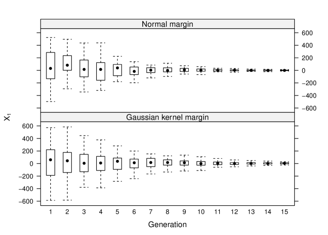
   Figure 2: Box-plots illustrating the evolution of the first variable of Griewank in the selected population of UMDA${}_{\textrm{g}}$ (top) and UMDA_e (bottom) for 15 generations.

   

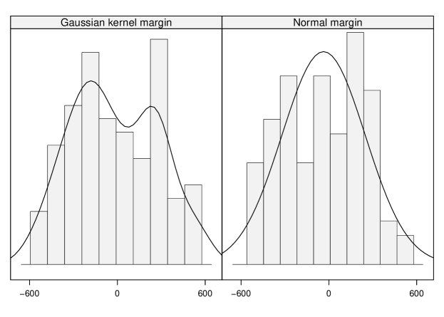
   Figure 3: Histograms of the first variable of the Griewank function in the selected population of the second generation with UMDA${}_{\textrm{e}}$ (left) and UMDA${}_{\textrm{g}}$ (right). The empirical and normal densities are superposed, respectively.

2. With asymmetric intervals, GCEDA with normal kernel margins is much better than with normal margins.

   With symmetric intervals, UMDA and GCEDA with normal margins behave better than with normal kernel margins. However, if the initial population is sampled asymmetrically, this situation changes, which is more remarkable in GCEDA (even GCEDA${}_{\textrm{g}}$ might not converge). This situation is illustrated in the optimization of the Griewank function with GCEDA${}_{\textrm{g}}$ and GCEDA${}_{\textrm{e}}$. Figure 4 shows both the normal and normal kernel densities of the first variable, which are estimated at generations $10$, $15$, $20$, $25$ and $30$. We recall that the zero value corresponds to the value of the variable in the global optimum. In Figure 4-(top), note that with normal margins the zero is located at the tail of the normal density, thus, it is sampled with low probability. As the evolution proceeds, the density moves away from zero. In Figure 4-(bottom), the normal kernel margins capture more local features of the distribution and it is more likely that good points are sampled.

   

   

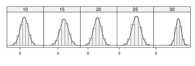
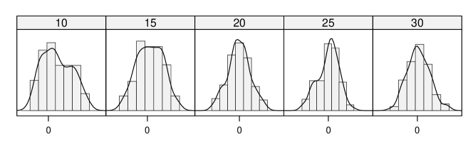
   Figure 4: Marginal distributions of the first variable of Griewank with GCEDA${}_{\textrm{g}}$ (top) and GCEDA${}_{\textrm{e}}$ (bottom) in the generations $10$, $15$, $20$, $25$ and $30$.

3. In problems where UMDA exhibits good performance, the introduction of correlations by GCEDA seems to be harmful.

   Sphere, Griewank and Ackley can be easily optimized by UMDA as far as the marginal information is enough for finding the global optimum. GCEDA requires to compute many parameters and larger populations are needed to estimate them reliably. Figure 5 illustrates this issue in the Sphere function. We run UMDA${}_{\textrm{g}}$ with its critical population. For GCEDA${}_{\textrm{g}}$ we use different population sizes, including the critical population of these two algorithms (86 and 325, respectively). The box-plot shows that GCEDA${}_{\textrm{g}}$ achieves the means and variances of UMDA${}_{\textrm{g}}$ but uses larger populations.

   

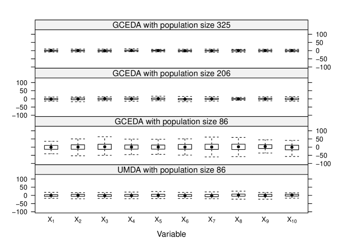
   Figure 5: Mean and variance of each variable in the selected population at $10^{th}$ generation with GCEDA${}_{\textrm{g}}$ and UMDA${}_{\textrm{g}}$ in Sphere. GCEDA${}_{\textrm{g}}$ requires larger populations than UMDA${}_{\textrm{g}}$.

4. UMDA is not capable of optimizing Summation Cancellation.

   Summation Cancellation has multivariate linear interactions between the variables [9]. As far as this information is essential for finding the global optimum, UMDA fails to optimize this function with both normal and kernel margins, while GCEDA is successful, though this algorithm is also sensitive to the effect of asymmetry.

Summarizing, we can say that both aspects: the statistical properties of the marginal distributions and the dependence structure play a crucial role for the success of EDA optimization. In the following sections we deal with the latter aspect.

4.3 Effect of the Dependence Structure

This section reports the most important results of our work. We investigate the effect of combining different copulas, applying the truncation strategy, and selecting the structure of C-vines and D-vines in the performance of VEDA.

4.3.1 Combining Different Bivariate Copulas

In this section we assess the effect of using different types of dependences when all the marginal distributions are normal. The experimental results obtained with CVEDA and DVEDA in Sphere, Griewank, Ackley and Summation Cancellation are presented in Tables 5–8, respectively. The studied algorithms are CVEDA${}_{\textrm{9, greedy, g}}$ and DVEDA${}_{\textrm{9, greedy, g}}$. The sub-indexes mean that they perform a complete construction of the vines ($9$ trees), use greedy heuristics to represent the stronger dependences in the first tree, and all margins are normal.

In the investigated problems the following hold:

Table 5: Results of VEDA in Sphere with $X_{i}\in[-600,600],\,i=1,\ldots,10$.

Algorithm	Success	Population	Evaluations	Best Evaluation
CVEDA${}_{\textrm{9, greedy, g}}$	$30/30$	$188$	$8,033.8\pm 170.5$	$6.8\textrm{E}-07\pm 2.1\textrm{E}-07$
DVEDA${}_{\textrm{9, greedy, g}}$	$30/30$	$207$	$8,818.2\pm 192.9$	$7.0\textrm{E}-07\pm 1.8\textrm{E}-07$

Table 6: Results of VEDA in Griewank with $X_{i}\in[-600,600],\,i=1,\ldots,10$.

Algorithm	Success	Population	Evaluations	Best Evaluation
CVEDA${}_{\textrm{9, greedy, g}}$	$30/30$	$213$	$9,151.9\pm 452.6$	$6.5\textrm{E}-07\pm 1.8\textrm{E}-07$
DVEDA${}_{\textrm{9, greedy, g}}$	$30/30$	$225$	$9,630.0\pm 309.2$	$6.9\textrm{E}-07\pm 1.5\textrm{E}-07$

Table 7: Results of VEDA in Ackley with $X{}_{i}\in[-30,30],\,i=1,\ldots,10$.

Algorithm	Success	Population	Evaluations	Best Evaluation
CVEDA${}_{\textrm{9, greedy, g}}$	$30/30$	$213$	$11,984.8\pm 184.9$	$7.9\textrm{E}-07\pm 1.5\textrm{E}-07$
DVEDA${}_{\textrm{9, greedy, g}}$	$30/30$	$213$	$11,920.9\pm 197.6$	$7.9\textrm{E}-07\pm 1.3\textrm{E}-07$

Table 8: Results of VEDA in Summation Cancellation with $X_{i}\in[-0,16,\,0,16],\,i=1,\ldots,10$.

Algorithm	Success	Population	Evaluations	Best Evaluation
CVEDA${}_{\textrm{9, greedy, g}}$	$30/30$	$625$	$84,958.3\pm 786.0$	$1.0\textrm{E}+05\pm 1.1\textrm{E}-07$
CVEDA${}_{\textrm{N, 9, greedy, g}}$	$30/30$	$319$	$43,373.3\pm 539.5$	$1.0\textrm{E}+05\pm 1.3\textrm{E}-07$
DVEDA${}_{\textrm{9, greedy, g}}$	$30/30$	$1400$	$161,840.0\pm 1,352.5$	$1.0\textrm{E}+05\pm 9.3\textrm{E}-08$
DVEDA${}_{\textrm{N, 9, greedy, g}}$	$30/30$	$488$	$58,494.9\pm 457.3$	$1.0\textrm{E}+05\pm 1.3\textrm{E}-07$

1. CVEDA and DVEDA exhibit a good performance in problems with both strong and weak dependences between the variables.

   While UMDA uses the independence model and GCEDA assumes a linear dependence structure, CVEDA and DVEDA do not assume the same type of dependence across all pairs of variables. The estimation procedures used by the vine-based algorithms select among a group of candidate bivariate copulas, the one that fits the data appropriately. CVEDA and DVEDA perform, in general, between UMDA and GCEDA in terms of the number of function evaluations.

2. CVEDA exhibits better results than DVEDA in easy problems for UMDA (Sphere, Griewank and Ackley).

   The model used by DVEDA allows a more freely selection of the bivariate dependences that will be explicitly modeled, while the model used by CVEDA has a more restrictive structure. These characteristics enable DVEDA to fit in the first tree a greater number of bivariate copulas that represent dependences. This may explain why DVEDA requires larger sample sizes than CVEDA, and thus more function evaluations.

3. CVEDA has much better results than DVEDA in Summation Cancellation.

   Summation Cancellation reaches its global optimum when the sum in the denominator of the fraction is zero. The $i$-th term of this sum is the sum of the first $i$ variables of the function. Thus, the first variables have a greater influence in the value of the sum. The selected populations reflect these characteristics including stronger associations between the first variables and the next ones. A C-vine structure provides a more appropriate modeling of this situation than a D-vine structure, since it is possible to find a variable that governs the interactions in the sample. However, as it was pointed out before, here the interesting issue is the success of GCEDA. The explanation is simple. On one hand, Summation Cancellation has multivariate linear interactions between the variables [9]. On the other hand, the multivariate normal distribution is indeed, a linear model of interactions.

4. Combining normal and non-normal copulas worsens the results of the vine-based algorithms in Summation Cancellation.

   Since the multivariate linear interactions of Summation Cancellation are readily modeled with a multivariate normal dependence structure, GCEDA has better performance than vine-based EDAs, which can fit copulas of different families (Tables 4 and 8). We repeated the experiments using only product and normal copulas. The results show similar performance of CVEDA${}_{\textrm{N, 9, greedy, g}}$, DVEDA${}_{\textrm{N, 9, greedy, g}}$ and GCEDA, being CVEDA slightly better than DVEDA.

Regarding the results presented in this section, we can summarize that EDAs using pair-copula constructions exhibit a more robust behavior than EDAs using multivariate product or normal copula in the given set of benchmark functions.

4.3.2 Truncation of C-vines and D-vines

In order to reduce the number of levels of the pair-copula decompositions, and hence simplify the constructions, we apply two different approaches: the truncation level is given as a parameter or it is determined by a model selection procedure based on AIC or BIC (see Section 3.3.1). We study the effect of both strategies in the Sphere and Summation Cancellation functions, as examples of problems with week and strong correlated variables. The following algorithms are compared:

• CVEDA${}_{\textrm{3, greedy, g}}$ and DVEDA${}_{\textrm{3, greedy, g}}$ truncate the vines at the third tree.

• CVEDA${}_{\textrm{6, greedy, g}}$ and DVEDA${}_{\textrm{6, greedy, g}}$ truncate the vines at the sixth tree.

• CVEDA${}_{\textrm{AIC, greedy, g}}$ and DVEDA${}_{\textrm{AIC, greedy, g}}$ determine the required number of trees using AIC.

• CVEDA${}_{\textrm{BIC, greedy, g}}$ and DVEDA${}_{\textrm{BIC, greedy, g}}$ determine the required number of trees using BIC.

The results of the experiments in Sphere and Summation Cancellation are presented in Tables 9 and 10, respectively. The main results are summarized in the following points:

Table 9: Results of VEDA with truncation in Sphere with $X_{i}\in[-600,600],\,i=1,\ldots,10$.

Algorithm	Success	Population	Evaluations	Best Evaluation
CVEDA${}_{\textrm{3, greedy, g}}$	$30/30$	$175$	$7,536.6\pm 151.9$	$6.5\textrm{E}-07\pm 2.2\textrm{E}-07$
CVEDA${}_{\textrm{6, greedy, g}}$	$30/30$	$191$	$8,174.8\pm 176.6$	$6.7\textrm{E}-07\pm 1.9\textrm{E}-07$
CVEDA${}_{\textrm{AIC, greedy, g}}$	$30/30$	$163$	$7,106.8\pm 139.3$	$6.6\textrm{E}-07\pm 2.0\textrm{E}-07$
CVEDA${}_{\textrm{BIC, greedy, g}}$	$30/30$	$113$	$5,017.2\pm 134.6$	$6.8\textrm{E}-07\pm 1.6\textrm{E}-07$
DVEDA${}_{\textrm{3, greedy, g}}$	$30/30$	$191$	$8,149.3\pm 161.2$	$6.5\textrm{E}-07\pm 1.8\textrm{E}-07$
DVEDA${}_{\textrm{6, greedy, g}}$	$30/30$	$207$	$8,818.2\pm 128.6$	$6.9\textrm{E}-07\pm 1.8\textrm{E}-07$
DVEDA${}_{\textrm{AIC, greedy, g}}$	$30/30$	$163$	$6,992.7\pm 144.2$	$6.5\textrm{E}-07\pm 1.9\textrm{E}-07$
DVEDA${}_{\textrm{BIC, greedy, g}}$	$30/30$	$138$	$6,026.0\pm 127.2$	$7.0\textrm{E}-07\pm 2.2\textrm{E}-07$

Table 10: Results of VEDA with truncation in Summation Cancellation with $X_{i}\in[-0,16,\,0,16]$, $i=1,\ldots,10$.

Algorithm	Success	Population	Evaluations	Best Evaluation
CVEDA${}_{\textrm{3, greedy, g}}$	$0/30$	$2000$	$500,000.0\pm 0.0$	$2.6\textrm{E}+03\pm 3.4\textrm{E}+03$
CVEDA${}_{\textrm{6, greedy, g}}$	$0/30$	$2000$	$500,000.0\pm 0.0$	$3.7\textrm{E}+04\pm 3.2\textrm{E}+04$
CVEDA${}_{\textrm{AIC, greedy, g}}$	$30/30$	$650$	$90,003.3\pm 1,262.8$	$1.0\textrm{E}+05\pm 1.2\textrm{E}-07$
CVEDA${}_{\textrm{BIC, greedy, g}}$	$30/30$	$800$	$108,506.6\pm 1,647.3$	$1.0\textrm{E}+05\pm 9.8\textrm{E}-08$
DVEDA${}_{\textrm{3, greedy, g}}$	$0/30$	$2000$	$500,000.0\pm 0.0$	$8.4\textrm{E}+04\pm 2.5\textrm{E}+04$
DVEDA${}_{\textrm{6, greedy, g}}$	$10/30$	$2000$	$412,133.3\pm 12,8711.1$	$9.9\textrm{E}+04\pm 1.7\textrm{E}+02$
DVEDA${}_{\textrm{AIC, greedy, g}}$	$30/30$	$1300$	$152,750.0\pm 1,404.1$	$1.0\textrm{E}+05\pm 1.0\textrm{E}-07$
DVEDA${}_{\textrm{BIC, greedy, g}}$	$26/30$	$2000$	$285,000.0\pm 100,221.0$	$9.9\textrm{E}+04\pm 6.9\textrm{E}-03$

1. The algorithms that use the truncation strategy based on AIC or BIC exhibit a more robust behavior.

   The necessary number of trees depends on the characteristics of the function being optimized. In the Sphere function, a small number of trees is quite enough, while in Summation Cancellation it is preferable to expand the pair-copula decomposition completely. In both functions the better results are obtained when the truncation level is determined by a model selection procedure based on AIC or BIC, since cutting the model arbitrarily could cause that important dependences are not represented. The latter was the strategy applied in [40], where a D-vine with normal copulas was only expanded up to the second tree. A combination of both strategies could be an appropriate solution.

2. For VEDA the truncation method based on AIC is preferable than the truncation based on BIC.

   In the Sphere function, the vine-based EDAs that use truncation based on BIC perform better than those based on AIC. The opposite occurs in Summation Cancellation, where DVEDA${}_{\textrm{BIC, greedy, g}}$ fail in the $30$ runs. Both situations are caused by the term that penalizes the number of parameters in these metrics. BIC prefers models with less number of copulas than AIC [10], which is good for Sphere, but compromises the convergence of the algorithms in Summation Cancellation. The algorithms using AIC have a good performance in both functions. Specifically, in Sphere the number of trees was never greater than three with CVEDA and four with DVEDA; in Summation Cancellation both algorithms perform complete construction of the vines (nine trees).

In the following section, we study the importance of the selection of the bivariate dependences explicitly modeled in the first tree of C-vines and D-vines.

4.3.3 Selection of the Structure of C-vines and D-vines

The aim of this section is to assess the importance of selecting an appropriate ordering of the variables in the pair-copula decomposition for the optimization with vine-based EDAs.

Here we repeat the experiments with Sphere and Summation Cancellation, but this time the variables in the first tree in the decomposition are ordered randomly instead of representing the strongest bivariate dependences. The instances of the algorithms selected in these experiments are those that showed the best performance in the truncation experiments of the previous section. The results are presented in Tables 11 and 12.

Table 11: Results of VEDA with a random selection of the structure of the first tree of the vines at each generation in Sphere with $X{}_{i}\in[-600,600],\,i=1,\ldots,10$.

Algorithm	Success	Population	Evaluations	Best Evaluation
CVEDA${}_{\textrm{BIC, random, g}}$	$30/30$	$100$	$4,523.3\pm 100.6$	$6.9\textrm{E}-07\pm 1.8\textrm{E}-07$
DVEDA${}_{\textrm{BIC, random, g}}$	$30/30$	$100$	$4,526.6\pm 114.2$	$6.6\textrm{E}-07\pm 1.6\textrm{E}-07$

Table 12: Results of VEDA with a random selection of the structure of the first tree of the vines at each generation in Summation Cancellation with $X_{i}\in[-0,16,\,0,16],\,i=1,\ldots,10$.

Algorithm	Success	Population	Evaluations	Best Evaluation
CVEDA${}_{\textrm{AIC, random, g}}$	$30/30$	$775$	$110,360.0\pm 2,020.9$	$1.0\textrm{E}+05\pm 1.1\textrm{E}-07$
DVEDA${}_{\textrm{AIC, random, g}}$	$30/30$	$1500$	$255,900.0\pm 5,205.7$	$1.0\textrm{E}+05\pm 1.2\textrm{E}-07$

In the Sphere function, the algorithms that use a random structure exhibit a better performance, since the number of product copulas that are fitted is greater. In this case, the estimated model resembles independence model used by UMDA, which indeed exhibits the best performance with the Sphere function. The opposite occurs with Summation Cancellation, where the use of a random structure in the first tree causes that important correlations for an efficient search are not represented, which deteriorates the performance of the algorithms in terms of the number of function evaluations. The main conclusion of this part is that it is necessary to make a careful selection of the structure of the pair-copula decomposition. The representation of the strongest dependences is important in order to construct more robust vine-based EDAs.

5 Conclusions

This paper introduces a class of EDAs called VEDAs. Two algorithms of this class are presented: CVEDA and DVEDA, which model the search distributions using C-vines and D-vines, respectively.

The copula EDAs based on vines are more flexible than those based on the multivariate product and normal copulas, because the PCC models can describe a richer variety of dependence patterns. Our empirical investigation confirms the robustness of CVEDA and DVEDA in both strong and weak correlated problems.

We have found that building the complete structure of the vine is not always necessary. However, cutting the model at a tree selected arbitrarily could cause that important dependences are not represented. A more appropriate global strategy could be to combine setting a maximum number of trees with a model selection technique, such as the truncation method based on AIC or BIC. We also found that it is important to make a conscious selection of the pairwise dependences represented explicitly in the model.

Our findings show that both the statistical properties of the margins and the dependence structure play a crucial role in the success of optimization. The use of copulas and vines in EDAs represents a new way to deal with more flexible search distributions and different sources of complexity that arise in optimization.

As future research we consider to extend the class of VEDAs with regular vines. Our algorithms have been used in the optimization of test functions, such as the ones proposed in CEC 2005 benchmark [47]. In general, these functions display independence or linear correlations. In the future, we will seek problems with relevant dependences to the vine models studied in this work.

Appendix A Expressions of the $h$ and $h^{-1}$ Functions of Various Bivariate Copulas

The pair-copulas used in this work are product, normal, Student’s $t$, Clayton, rotated Clayton, Gumbel and rotated Gumbel. This appendix contains the definition of these copulas and the $h$ and $h^{-1}$ functions required to use this copulas in pair-copula constructions.

The Bivariate Product Copula

An immediate consequence of Sklar’s theorem is that two random variables are independent if and only if their underlying copula is $C_{\textrm{I}}\left(u,v\right)=uv$. For this copula $h_{\textrm{I}}(x,v)=x$ and $h_{\textrm{I}}^{-1}(u,v)=u$.

The Bivariate Normal Copula

The distribution function of the bivariate normal copula is given by

$$C_{\textrm{N}}(u,v;\rho)=\Phi_{\rho}(\Phi^{-1}(u),\Phi^{-1}(v)),$$

where $\Phi_{\rho}$ is the bivariate normal distribution function with correlation parameter $\rho$ and $\Phi^{-1}$ is the inverse of the standard univariate normal distribution function. For this copula the $h$ and $h^{-1}$ functions are

$$h_{\textrm{N}}\left(x,v;\rho\right)=\Phi\left(\frac{\Phi^{-1}\left(x\right)-\rho\,\Phi^{-1}\left(v\right)}{\sqrt{1-\rho^{2}}}\right),$$

$$h_{\textrm{N}}^{-1}\left(u,v;\rho\right)=\Phi\left(\Phi^{-1}\left(u\right)\sqrt{1-\rho^{2}}+\rho\,\Phi^{-1}\left(v\right)\right).$$

The derivation of these formulas are given in [1].

The Bivariate Student’s $t$ Copula

The distribution function of the bivariate Student’s $t$ copula is given by

$$C_{\textrm{t}}(u,v;\rho,\nu)=t_{\rho,\nu}(t_{\nu}^{-1}(u),t_{\nu}^{-1}(v)),$$

where $t_{\rho,\nu}$ is the distribution function of the bivariate Student’s $t$ distribution with correlation parameter $\rho$ and $\nu$ degrees of freedom and $t_{\nu}^{-1}$ is the inverse of the univariate Student’s $t$ distribution function with $\nu$ degrees of freedom. For this copula the $h$ and $h^{-1}$ functions are

$$h_{\textrm{t}}\left(x,v;\rho,\nu\right)=t_{\nu+1}\left(\frac{t_{\nu}^{-1}\left(x\right)-\rho\,t_{\nu}^{-1}\left(v\right)}{\sqrt{\frac{\left(\nu+\left(t_{\nu}^{-1}\left(v\right)\right)^{2}\right)\left(1-\rho^{2}\right)}{\nu+1}}}\right),$$

$$h_{\textrm{t}}^{-1}\left(u,v;\rho,\nu\right)=t_{v}\left(t_{v+1}^{-1}\left(u\right)\sqrt{\frac{\left(\nu+\left(t_{\nu}^{-1}\left(v\right)\right)^{2}\right)\left(1-\rho^{2}\right)}{\nu+1}}+\rho\,t_{\nu}^{-1}\left(v\right)\right).$$

The derivation of these formulas are given in [1].

The Bivariate Clayton Copula

The distribution function of the bivariate Clayton copula is given by

$$C_{\textrm{C}}\left(u,v;\theta\right)=\left(u^{-\theta}+v^{-\theta}-1\right)^{-1/\theta},$$ (8)

where $\theta>0$ is a parameter controlling the dependence. Perfect dependence is obtained when $\theta\rightarrow\infty$, while $\theta\rightarrow 0$ implies independence. For this copula the $h$ and $h^{-1}$ functions are

$$h_{\textrm{C}}\left(x,v;\theta\right)=v^{-\theta-1}\left(x^{-\theta}+v^{-\theta}-1\right)^{-1-1/\theta},$$

$$h_{\textrm{C}}^{-1}\left(u,v;\theta\right)=\left(\left(uv^{\theta+1}\right)^{-\theta/(\theta+1)}+1-v^{-\theta}\right)^{-1/\theta}.$$

The derivation of these formulas are given in [1].

The Bivariate Rotated Clayton Copula

The bivariate Clayton copula, as defined in (8), can only capture positive dependence. Following the transformation used in [10], we consider a $90$ degrees rotated version of this copula. The distribution function of the bivariate rotated Clayton copula is obtained as

$$C_{\textrm{RC}}(u,v;\theta)=u-C_{\textrm{C}}(u,1-v;-\theta),$$

where $\theta<0$ is a parameter controlling the dependence and $C_{\textrm{C}}$ denotes the distribution function of the bivariate Clayton copula. For this copula the $h$ and $h^{-1}$ functions are

$$h_{\textrm{RC}}(x,v;\theta)=h_{\textrm{C}}(x,1-v;-\theta)$$

and

$$h_{\textrm{RC}}^{-1}(u,v;\theta)=h_{\textrm{C}}^{-1}(u,1-v;-\theta),$$

where $h_{\textrm{C}}$ and $h_{\textrm{C}}^{-1}$ denote the expressions of the $h$ and $h^{-1}$ functions for the bivariate Clayton copula.

The Bivariate Gumbel Copula

The distribution function of a bivariate Gumbel copula is given by

$$C_{\textrm{G}}(u,v;\theta)=\exp\left(-\left(\left(-\log\,u\right)^{\theta}+\left(-\log\,v\right)^{\theta}\right)^{1/\theta}\right),$$

where $\theta\geq 1$ is a parameter controlling the dependence. Perfect dependence is obtained when $\theta\rightarrow\infty$, while $\theta=1$ implies independence. The $h$ function is

$$h_{G}\left(x,v;\theta\right)=C_{G}\left(x,v;\theta\right)\frac{1}{v}\left(-\log\,v\right)^{\theta-1}\left[\left(-\log\,x\right)^{\theta}+\left(-\log\,v\right)^{\theta}\right]^{1/\theta-1},$$

but $h_{\textrm{G}}^{-1}$ cannot be written in closed form; therefore, we obtain it numerically using Brent’s method [11]. The derivation of these formulas are given in [1].

The Bivariate Rotated Gumbel Copula

The bivariate Gumbel copula can only represent positive dependence. As for the bivariate Clayton copula and following the transformation used in [10], we also consider a $90$ degrees rotated version of the bivariate Gumbel copula. The distribution function of the bivariate rotated Gumbel copula is defined as

$$C_{\textrm{RG}}(u,v;\theta)=u-C_{G}(u,1-v;-\theta),$$

where $\theta<-1$ is a parameter controlling the dependence and $C_{\textrm{G}}$ denotes the distribution function of the bivariate Gumbel copula. For this copula the $h$ and $h^{-1}$ functions are

$$h_{\textrm{RG}}(x,v;\theta)=h_{\textrm{G}}(x,1-v;-\theta)$$

and

$$h_{\textrm{RG}}^{-1}(u,v;\theta)=h_{\textrm{G}}^{-1}(u,1-v;-\theta),$$

where $h_{\textrm{G}}$ and $h_{\textrm{G}}^{-1}$ denote the expressions of the $h$ and $h^{-1}$ functions for the bivariate Gumbel copula.

References

- [1] K. Aas, C. Czado, A. Frigessi, and H. Bakken. Pair-copula constructions of multiple dependence. Insurance: Mathematics and Economics, 44(2):182–198, 2009.
- [2] H. Akaike. A new look at statistical model identification. IEEE Transactions on Automatic Control, 19:716–723, 1974.
- [3] R. J. Arderí. Algoritmo con estimación de distribuciones con cópula gaussiana. Bachelor thesis, University of Havana, Cuba, June 2007.
- [4] A. Azzalini. A note on the estimation of a distribution function and quantiles by a kernel method. Biometrika, 68(1):326–328, 1981.
- [5] T. Bedford and R. M. Cooke. Monte Carlo simulation of vine dependent random variables forapplications in uncertainty analysis. In Proceedings of ESREL 2001, Turin, Italy, 2001.
- [6] T. Bedford and R. M. Cooke. Probability density decomposition for conditionally dependent random variables modeled by vines. Annals of Mathematics and Artificial Intelligence, 32(1):245–268, 2001.
- [7] T. Bedford and R. M. Cooke. Vines — a new graphical model for dependent random variables. The Annals of Statistics, 30(4):1031–1068, 2002.
- [8] E. Bengoetxea, T. Miquélez, J. A. Lozano, and P. Larrañaga. Experimental results in function optimization with EDAs in continuous domain. In P. Larrañaga and J. A. Lozano, editors, Estimation of Distribution Algorithms. A New Tool for Evolutionary Computation, pages 181–194. Kluwer Academic Publisher, 2002.
- [9] P. A. N. Bosman and D. Thierens. Numerical optimization with real-valued estimation of distribution algorithms. In M. Pelikan, K. Sastry, and E. Cantú-Paz, editors, Scalable Optimization via Probabilistic Modeling. From Algorithms to Applications, pages 91–120. Springer-Verlag, 2006.
- [10] E. C. Brechmann. Truncated and simplified regular vines and their applications. Diploma thesis, University of Technology, Munich, Germany, October 2010.
- [11] R. P. Brent. Algorithms for Minimization Without Derivatives. Prentice-Hall, 1973. ISBN 0-13-022335-2.
- [12] A. Cuesta-Infante, R. Santana, J. I. Hidalgo, C. Bielza, and P. Larrañaga. Bivariate empirical and -variate archimedean copulas in estimation of distribution algorithms. In Proceedings of the IEEE Congress on Evolutionary Computation (CEC 2010), pages 1355–1362, July 2010.
- [13] S. Demarta and A. J. McNeil. The t copula and related copulas. International Statistical Review, 73(1):111–129, 2005.
- [14] L. Devroye. Non-Uniform Random Variate Generation. Springer-Verlag, 1986. ISBN 0-387-96305-7.
- [15] D. Fantazzini. Three-stage semi-parametric estimation of t-copulas: Asymptotics, finite-sample properties and computational aspects. Computational Statistics and Data Analysis, 54:2562–2579, 2010.
- [16] G. Fusai and A. Roncoroni. Implementing Models in Quantitative Finance: Methods and Cases, chapter Structuring Dependence Using Copula Functions, pages 231–267. Springer-Verlag, 2008.
- [17] Y. Gao. Multivariate estimation of distribution algorithm with Laplace transform archimedean copula. In W. Hu and X. Li, editors, Proceedings of the International Conference on Information Engineering and Computer Science (ICIECS 2009), December 2009.
- [18] C. Genest and A. C. Favre. Everything you always wanted to know about copula modeling but were afraid to ask. Journal of Hydrologic Engineering, 12(4):347–368, 2007.
- [19] C. Genest and B. Rémillard. Tests of independence or randomness based on the empirical copula process. Test, 13(2):335–369, 2004.
- [20] C. Genest, B. Rémillard, and D. Beaudoin. Goodness-of-fit tests for copulas: A review and a power study. Insurance: Mathematics and Economics, 44:199–213, 2009.
- [21] Y. González-Fernández. Algoritmos con estimación de distribuciones basados en cópulas y vines. Bachelor thesis, University of Havana, Cuba, June 2011.
- [22] Y. González-Fernández, D. Carrera, M. Soto, and A. Ochoa. Vine estimation of distribution algorithm. In VIII Congreso Español sobre Metaheurísticas, Algoritmos Evolutivos y Bioinspirados (MAEB 2012), February 2012. http://congresomaeb2012.uclm.es/papers/paper_99.pdf.
- [23] Y. González-Fernández and M. Soto. copulaedas: Estimation of Distribution Algorithms Based on Copulas, 2011. R package version 1.1.0. Available at http://CRAN.R-project.org/package=copulaedas.
- [24] Y. González-Fernández and M. Soto. vines: Multivariate Dependence Modeling with Vines, 2011. R package version 1.0.3. Available at http://CRAN.R-project.org/package=vines.
- [25] M. Hauschild and M. Pelikan. An introduction and survey of estimation of distribution algorithms. Swarm and Evolutionary Computation, 1:111–128, 2011.
- [26] H. Joe. Families of -variate distributions with given margins and bivariate dependence parameters. In L. Rüschendorf, B. Schweizer, and M. D. Taylor, editors, Distributions with fixed marginals and related topics, pages 120–141, 1996.
- [27] H. Joe. Multivariate Models and Dependence Concepts. Chapman & Hall, 1997.
- [28] S. Kern, S. D. Müller, N. Hansen, D. Büche, J. Ocenasek, and P. Koumoutsakos. Learning probability distributions in continuous evolutionary algorithms – A comparative review. Natural Computing, 3:77–112, 2003.
- [29] D. Kurowicka and R. M. Cooke. Uncertainty Analysis with High Dimensional Dependence Modelling. John Wiley & Sons, 2006. ISBN 978-0-470-86306-0.
- [30] D. Kurowicka and R. M. Cooke. Sampling algorithms for generating joint uniform distributions using the vine-copula method. Computational Statistics & Data Analysis, 51:2889–2906, 2007.
- [31] P. Larrañaga and J. A. Lozano, editors. Estimation of Distribution Algorithms: A New Tool for Evolutionary Computation, volume 2 of Genetic Algorithms and Evolutionary Computation. Kluwer Academic Publisher, 2002. ISBN 978-0-7923-7466-4.
- [32] H. Mühlenbein and T. Mahnig. FDA — a scalable evolutionary algorithm for the optimization of additively decomposed functions. Evolutionary Computation, 7(4):353–376, 1999.
- [33] H. Mühlenbein and G. Paaß. From recombination of genes to the estimation of distributions i. Binary parameters. In Parallel Problem Solving from Nature — PPSN IV, pages 178–187. Springer-Verlag, 1996.
- [34] R. B. Nelsen. An Introduction to Copulas. Springer-Verlag, 2 edition, 2006. ISBN 978-0387-28659-4.
- [35] M. Pelikan. Hierarchical Bayesian Optimization Algorithm. Toward a New Generation of Evolutionary Algorithms. Springer-Verlag, 2005.
- [36] R Development Core Team. R: A Language and Environment for Statistical Computing. R Foundation for Statistical Computing, Vienna, Austria, 2011. ISBN 3-900051-07-0. http://www.R-project.org/.
- [37] D. J. Rosenkrantz, R. E. Stearns, and P. M. Lewis II. An analysis of several heuristics for the traveling salesman problem. SIAM Journal on Computing, 6(3):563–581, 1977.
- [38] P. Rousseeuw and G. Molenberghs. Transformation of nonpositive semidefinite correlation matrices. Communications in Statistics: Theory and Methods, 22:965–984, 1993.
- [39] R. Salinas-Gutiérrez, A. Hernández-Aguirre, and E. Villa-Diharce. Using copulas in estimation of distribution algorithms. In Proceedings of the Eight Mexican International Conference on Artificial Intelligence (MICAI 2009), pages 658–668, November 2009.
- [40] R. Salinas-Gutiérrez, A. Hernández-Aguirre, and E. Villa-Diharce. D-vine EDA: A new estimation of distribution algorithm based on regular vines. In Proceedings of the Genetic and Evolutionary Computation Conference (GECCO 2010), pages 359–365, July 2010.
- [41] G. Schwarz. Estimating the dimension of a model. The Annals of Statistics, 6:461–464, 1978.
- [42] B. W. Silverman. Density Estimation for Statistics and Data Analysis. Chapman & Hall, 1986.
- [43] A. Sklar. Fonctions de répartition à dimensions et leurs marges. Publications de l’Institut de Statistique de l’Université de Paris, 8:229–231, 1959.
- [44] M. Soto and Y. González-Fernández. Vine estimation of distribution algorithms. Technical Report ICIMAF 2010-561, Institute of Cybernetics, Mathematics and Physics, Cuba, May 2010. ISSN 0138-8916.
- [45] M. Soto, A. Ochoa, and R. J. Arderí. Gaussian copula estimation of distribution algorithm. Technical Report ICIMAF 2007-406, Institute of Cybernetics, Mathematics and Physics, Cuba, June 2007. ISSN 0138-8916.
- [46] M. Soto, A. Ochoa, Y. González-Fernández, Y. Milanés, A. Álvarez, D. Carrera, and E. Moreno. Vine estimation of distribution algorithms with application to molecular docking. In S. Shakya and R. Santana, editors, Markov Networks in Evolutionary Computation, volume 14 of Adaptation, Learning, and Optimization, pages 209–225. Springer-Verlag, 2012. ISBN 978-3-642-28899-9.
- [47] P. N. Suganthan, N. Hansen, J. J. Liang, K. Deb, Y.-P. Chen, A. Auger, and S. Tiwari. Problem definitions and evaluation criteria for the CEC 2005 special session on real-parameter optimization. Technical report, Nanyang Technological University, Singapore, May 2005.
- [48] L. Wang, J. Zeng, and Y. Hong. Estimation of distribution algorithm based on copula theory. In Proceedings of the IEEE Congress on Evolutionary Computation (CEC 2009), pages 1057–1063, May 2009.