Constraining the luminosity function parameters and population size of radio pulsars in globular clusters

Abstract

The luminosity distribution of Galactic radio pulsars is believed to be log-normal in form. Applying this functional form to populations of pulsars in globular clusters, we employ Bayesian methods to explore constraints on the mean and standard deviation of the function, as well as the total number of pulsars in the cluster. Our analysis is based on an observed number of pulsars down to some limiting flux density, measurements of flux densities of individual pulsars, as well as diffuse emission from the direction of the cluster. We apply our analysis to Terzan 5 and demonstrate, under reasonable assumptions, that the number of potentially observable pulsars is in a 95.45% credible interval of 133${}^{+101}_{-58}$. Beaming considerations would increase the true population size by approximately a factor of two.

1 Introduction

Globular clusters have high core stellar number densities that favour the formation of low-mass X-ray binaries (LMXBs) that are believed to be the progenitors of millisecond pulsars (MSPs; [Alpar et al. (1982), Alpar et al. 1982]). MSPs can be considered long-lived tracers of LMXBs, so constraints on the MSP content provide unique insights into binary evolution and the integrated dynamical history of globular clusters, while determining the radio luminosity function of these pulsars helps shed light on their emission mechanism.

[Faucher-Giguère & Kaspi (2006), Faucher-Giguère & Kaspi (2006)] have shown that the luminosity distribution of non-recycled Galactic pulsars appears to be log-normal in form. More recently, [Bagchi et al. (2011), Bagchi et al. (2011)] have verified that the observed luminosities of recycled pulsars in globular clusters are consistent with this result. Assuming, therefore, that there is no significant difference between the nature of Galactic and cluster populations, we use Bayesian techniques to investigate some of the consequences that occur when one applies this functional form to populations of pulsars in individual clusters. We are interested in the situation where we observe $n$ pulsars with luminosities above some limiting luminosity. There is a family of luminosity function parameters ($\mu$, $\sigma$) and population sizes ($N$) that is consistent with this observation, and here we analyze the posterior probabilities of different members of this family given the data. In our case, the data are the individual pulsar flux densities that we call $\{S_{i}\}$, the observed number of pulsars, $n$ and the total diffuse flux density of the cluster, $S_{\rm obs}$.

2 Bayesian parameter estimation

Luminosity and flux density are related by the standard pseudo-luminosity equation $L=S~{}r^{2}$, where $r$ is the distance to the pulsar (see [Lorimer & Kramer (2005), Lorimer & Kramer 2005]). This implies that the luminosity function is corrupted by uncertainties in distance. To mitigate this, we decided to perform our analysis initially in terms of the measured flux densities, and use a model of distance uncertainty to convert our results to the luminosity domain. We take the distance to all pulsars in a cluster to be the same. The log-normal in luminosity can then alternatively be written in terms of flux density. The probability of detecting a pulsar with flux density $S$ in the range $\log S$ to $\log S+d(\log S)$ is given by a log-normal in $S$ as

$$p(\log S)~{}d(\log S)=\frac{1}{\sigma_{S}\sqrt{2\pi}}e^{-\frac{(\log S-\mu_{S})^{2}}{2\sigma_{S}^{2}}}~{}d(\log S),$$ (1)

where $S$ is in mJy, and $\mu_{S}$ and $\sigma_{S}$ are the mean and standard deviation of the flux density distribution. The probability of observing a pulsar above the limit $S_{\rm min}$ is then

$$p_{\rm obs}=\int_{\log S_{\rm min}}^{\infty}p(\log S)~{}d(\log S)=\frac{1}{2}~{}{\rm erfc}\left(\frac{\log S_{\rm min}-\mu_{S}}{\sqrt{2}\sigma_{S}}\right).$$ (2)

First, we consider as data the measured flux densities of pulsars in the cluster, $\{S_{i}\}$. Ideally, the survey sensitivity limit $S_{\rm min}$ can be taken as another datum, but its exact value is not always known, so we decided to parametrize $S_{\rm min}$. The likelihood of observing a set of pulsars with fluxes $\{S_{i}\}$ is represented as

$$\prod\limits_{i=1}^{n}p_{i}(\log S_{i}|\mu_{S},\sigma_{S},S_{\rm min})=\prod\limits_{i=1}^{n}\frac{1}{p_{\rm obs}\sigma_{S}\sqrt{2\pi}}e^{-\frac{(\log S_{i}-\mu_{S})^{2}}{2\sigma_{S}^{2}}}$$ (3)

where $n$ is the number of observed pulsars in the cluster, and $p_{\rm obs}$ is as given in Equation (2). Uncertainties in the flux density measurements are not considered here, but it has to be noted that it will have the effect of underestimating the credible intervals on our posteriors.

To infer the total number of pulsars in the cluster, we follow [Boyles et al. (2011), Boyles et al. (2011)] to take as likelihood the probability of observing $n$ pulsars in a cluster with $N$ pulsars, given by the binomial distribution

$$p(n|N,\mu_{S},\sigma_{S},S_{\rm min})=\frac{N!}{n!(N-n)!}~{}p_{\rm obs}^{n}~{}(1-p_{\rm obs})^{N-n}.$$ (4)

Next, we incorporate information about the observed diffuse flux from the direction of the cluster. We assume that all radio emission is due to the pulsars in the cluster, both resolved and unresolved. For the likelihood of measuring the diffuse flux $S_{\rm obs}$, we choose

$$p(S_{\rm obs}|N,\mu_{S},\sigma_{S})=\frac{1}{\sigma_{\rm diff}\sqrt{2\pi}}~{}e^{-\frac{(S_{\rm obs}-S_{\rm diff})^{2}}{2\sigma_{\rm diff}^{2}}},$$ (5)

where $S_{\rm diff}$ is the expectation of the total diffuse flux of a cluster whose flux density distribution is a log-normal with parameters $\mu_{S}$ and $\sigma_{S}$, and having $N$ pulsars, and $\sigma_{\rm diff}$ is the standard deviation. Here, $S_{\rm diff}=N\langle S\rangle$ and $\sigma_{\rm diff}=\sqrt{N}~{}{\rm SD}(S)$ where the expectation of $S$ is given by $\langle S\rangle=10^{\mu_{S}+\frac{1}{2}\sigma_{S}^{2}\ln(10)}$ and the standard deviation of $S$, ${\rm SD}(S)=10^{\mu_{S}+\frac{1}{2}\sigma_{S}^{2}\ln(10)}\sqrt{10^{\sigma_{S}^{2}\ln(10)}-1}$. We do not consider the uncertainty in the diffuse flux measurement. The total likelihood, $p(\log S_{i},n,S_{\rm obs}|N,\mu_{S},\sigma_{S},S_{\rm min})$ is the product of the three likelihoods computed above.

The flux density distribution of pulsars in a cluster is not suitable for comparing the populations in different clusters, as it depends on the distance to the cluster. So we transform the total likelihood obtained in the previous subsection to the luminosity domain. Taking into account the uncertainty in distance as a distribution of distances, $p(r)$, it can be shown that the total likelihood in the luminosity domain is

$$p(\log S_{i},n,S_{\rm obs}|N,\mu,\sigma,S_{\rm min},r)=p(\log S_{i},n,S_{\rm obs}|N,\mu_{S},\sigma_{S},S_{\rm min}),$$ (6)

where $\mu$ and $\mu_{S}$ are related additively by the term $2\log r$, and $\sigma$ and $\sigma_{S}$ are equal. The final joint posterior in luminosity is then given by

$$\begin{split}p(N,&\mu,\sigma,S_{\rm min},r|\log S_{i},n,S_{\rm obs})\\ \propto~{}&p(\log S_{i},n,S_{\rm obs}|N,\mu,\sigma,S_{\rm min},r)~{}p(N)~{}p(\mu)~{}p(\sigma)~{}p(S_{\rm min})~{}p(r).\end{split}$$ (7)

The prior on $N$ is taken to be uniform from $n$ to $\infty$. We also use uniform priors on the model parameters $\mu$ and $\sigma$. We choose a uniform prior on $S_{\rm min}$ in the range (0, min($S_{i}$)], where the upper limit is the flux density of the least bright pulsar in the cluster. The prior on $r$ is taken to be a Gaussian. This joint posterior is integrated over various sets of model parameters to obtain marginalized posteriors.

3 Applications

We applied our Bayesian technique to Terzan 5. Although Terzan 5 has 34 known pulsars (Ransom S. M., private communication), we take $n=25$, the number of pulsars for which we have flux density measurements. The flux densities of the individual pulsars were collected in a literature survey ([Bagchi et al. (2011), Bagchi et al. 2011] and references therein). The flux densities we used were scaled from those reported at 1950 MHz by [Ransom et al. (2005), Ransom et al. (2005)] and [Hessels et al. (2006), Hessels et al. (2006)] to 1400 MHz using a spectral index, $\alpha=-1.9$, using the power law $S(\nu)\propto\nu^{\alpha}$. The observed diffuse flux density at 1400 MHz is taken to be $S_{\rm obs}=5.2$ mJy ([Fruchter & Goss (2000), Fruchter & Goss 2000]). The prior on $N$ was chosen to be uniform in [$n$, 500], which is sufficiently wide to ensure that the posterior does not rail against the prior boundaries. We chose uniform distributions in the same range of $\mu$ and $\sigma$ as used by [Bagchi et al. (2011), Bagchi et al. (2011)] as our priors. We took $S_{\rm min}$ to be uniform in (0, min($S_{i}$)]. The most recent measurement of the distance to Terzan 5, $r=5.5\pm 0.9$ kpc ([Ortolani et al. (2007), Ortolani et al. 2007]), was used to model the distance prior as a Gaussian. Figure 1 shows the results of the analysis. The median values of the three parameters with 95.45% credible intervals are: $N=92^{+318}_{-64}$, $\mu=-0.9^{+1.2}_{-1.1}$ and $\sigma=0.9^{+0.3}_{-0.4}$.

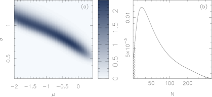
Figure 1: Results of the analysis for Terzan 5. For (a) and (b), the analysis was run with wide priors on $\mu$ and $\sigma$, with the ranges equal to those used by [Bagchi et al. (2011), Bagchi et al. (2011)], their Figure 2. (a) depicts the joint posterior on $\mu$ and $\sigma$, marginalized over $N$, $S_{\rm min}$ and $r$; (b) is the marginalized posterior for $N$. (c) Posterior on $N$ after applying narrow priors on $\mu$ and $\sigma$. In (b) and (c), the shaded regions lie outside a 95.45% credible interval.

Note that $N$ is the size of the population of pulsars that are beaming towards the Earth. Uncertainties notwithstanding, the beaming fraction of MSPs is generally thought to be $>$ 50% ([Kramer et al. (1998), Kramer et al. 1998]). This, together with the fact that most pulsars in globular clusters are MSPs, imply that the true population size in a cluster is approximately a factor of two more than the potentially observable population size.

3.1 Using prior information

In the framework developed in the previous section, we use broad uniform (non-informative) priors for the mean and standard deviation of the log-normal. This lack of prior information is apparent in Figure 1(b), where $N$ is not very well constrained. Prior information can help better constrain the parameters of interest. [Boyles et al. (2011), Boyles et al. (2011)] use models of Galactic pulsars from [Ridley & Lorimer (2010), Ridley & Lorimer (2010)] to narrow down $\mu$ to between $-$1.19 and $-$1.04, and $\sigma$ to the range 0.91 to 0.98. We have chosen our priors on $\mu$ and $\sigma$ to be uniform within these ranges. Applying the Bayesian analysis over this narrower range of $\mu$ and $\sigma$ results in much tighter constraints on $N$ as seen in Figure 1(c), where $N=133^{+101}_{-58}$. This result is consistent with that of [Bagchi et al. (2011), Bagchi et al. (2011)].

4 Conclusions

The technique described here would be useful in future studies of the globular cluster luminosity function where ongoing and future pulsar surveys are expected to provide a substantial increase in the number of known pulsars in many clusters. We anticipate that the increased amount of data would enable us to constrain the distributions of $\mu$ and $\sigma$ independently (i.e. without the need to assume prior information from the Galactic pulsar population). Further interferometric measurements of the diffuse radio flux in many clusters could provide improved constraints on $\mu$ and $\sigma$ by measuring the flux contribution from the individually unresolvable population of pulsars.

References

- [Alpar et al. (1982)] Alpar, M. A., Cheng, A. F., Ruderman, M. A., & Shaham, J. 1982, Nature, 300, 728
- [Bagchi et al. (2011)] Bagchi, M., Lorimer, D. R., & Chennamangalam, J. 2011, MNRAS, 418, 477
- [Boyles et al. (2011)] Boyles, J., Lorimer, D. R., Turk, P. J., Mnatsakanov, R., Lynch, R. S., Ransom, S. M., Freire, P. C., & Belczynski, K. 2011, ApJ, 742, 51