Braiding of non-Abelian anyons using pairwise interactions

Abstract

The common approach to topological quantum computation is to implement quantum gates by adiabatically moving non-Abelian anyons around each other. Here we present an alternative perspective based on the possibility of realizing the exchange (braiding) operators of anyons by adiabatically varying pairwise interactions between them rather than their positions. We analyze a system composed by four anyons whose couplings define a T-junction and we show that the braiding operator of two of them can be obtained through a particular adiabatic cycle in the space of the coupling parameters. We also discuss how to couple this scheme with anyonic chains in order to recover the topological protection.

I Introduction

The purpose of topological quantum computation (TQC) is to realize a reliable quantum computer, exploiting the existence of special quasiparticles, known as non-Abelian anyons, in certain exotic condensed matter systems kitaev03 ; nayak08 . The presence of several such particles gives rise to degenerate ground states which cannot be distinguished by local measurements. The ground state manifold is then adopted as the computational space, and quantum gates can be performed by braiding (exchanging the positions of the anyons), as shown in Fig. 1a). The resulting unitary transformation of the wave function depends only on the order of the exchanges and not on the details of their paths, thus these quantum gates are said to be topologically protected. In the standard scheme of TQC nayak08 , there are two main ingredients needed to implement braiding. First, it must be possible to change the positions of anyons in such a way that the wave function of the system always belongs to the space of the degenerate ground states. Second, at all stages of the braiding the interactions between the anyons used for the computation must be negligible in order to preserve the degeneracy of the ground states and to avoid the presence of non-adiabatic time-dependent phases. This requires the anyons to be well separated in space.

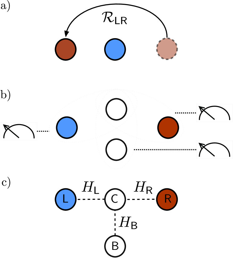
Figure 1: Different ways to braid quasiparticles in topological quantum computation. Panel (a): the original scheme for braiding, where quantum gates are obtained by moving the non-Abelian quasiparticles (red and blue dots) one around the other. Panel (b): measurement-only TQC, in which ancillary anyons are added to the system (white dot), and quantum gates are obtained as a sequence of non-demolition pairwise measurements (represented by the dashed ellipses) which induce teleportation of the computational anyons through the ancillary ones. Panel (c): the interaction-based braiding, which makes use of the interaction between computational and ancillary anyons in a T-junction geometry.

The possibility to realize braiding operators without moving the anyons was then introduced by Bonderson, Freedman and Nayak in Refs. bonderson08 ; bonderson09 . In their scheme, the measurement-only TQC, the braid operators are obtained as a result of a probabilistically determined sequence of non-demolition measurements of the computational anyons as shown in Fig. 1b). This measurement would rely, for example, on the non-Abelian edge state interferometry fradkin98 ; dassarma05 ; stern06 ; bonderson06 ; bonderson08-2 ; bishara09 , which has been actively developed both experimentally and theoretically overbosch07 ; bishara08 ; rosenow08 ; willett09 ; willett10 ; kang11 ; simon11 ; clarke11 ; willett12 .

A different way to braid non-Abelian anyons without moving them around each other has been theoretically developed in the case of Majorana fermions appearing at the ends of one-dimensional topological superconductors Kit01 ; Lut10 ; Ore10 . Initially, it was shown in Ref. Ali11 how braids can be realized in wire networks by moving the Majorana fermions through T-shaped junctions. In this case, the movement of the quasiparticles is restricted to a quasi one-dimensional system, thus relaxing the limitation of braiding to two dimensions. Subsequent proposals however have eliminated the need to physically move the topological defects altogether, showing how the same ground state transformations can be implemented using the mutual interactions between Majoranas, controlling either tunnel couplings via gate voltages Sau11 or capacitive couplings via magnetic fluxes vanheck11 . Finally, in Ref. hal12 a general theory of adiabatic manipulations of Majorana fermions in nanowires was formulated. Unless we allow for physically bending and rotating the wires, the minimal setup required for the braid operation is a T-shaped configuration of nanowires where a central Majorana is coupled to at least three neighbors. The evolution over a path in parameter space results in the same non-Abelian Berry phase expected after an exchange of two quasiparticles in real space.

In this paper, we aim to show that in a broad range of anyonic models braiding is not only a property of the particle motion, but it is also encoded in the many-body Hamiltonian of coupled anyons. We will show how it is possible to engineer effective braidings by manipulating mutual couplings between neighboring anyons, rather than their coordinates in space. The motion of anyons is unnecessary also in measurement-only TQC, however our proposal is different because the braid operation is performed in a deterministic manner and does not rely on the procedure of anyon measurement.

The outline of the paper is the following. In Section II we present the minimal braiding setup, formed by four anyons in a T-shaped junction, and we give an expression of the interaction Hamiltonian in terms of the $\mathcal{F}$-matrices of a generic anyon model. In Sec. III we present in detail the adiabatic cycle in parameter space used to braid the non-Abelian anyons, while in Sec. IV we discuss how errors affecting the adiabatic evolution can be reduced by embedding the braiding junction in a bigger system of anyon chains and conclude.

II The T-junction

We consider a system of four anyons with the same topological charge t in a T-junction geometry, with a central anyon (labeled $\mathsf{t_{C}}$) coupled to other three (labeled $\mathsf{t_{L}}$, $\mathsf{t_{R}}$, $\mathsf{t_{B}}$ for left, right and bottom), as shown in Fig. 1c and Fig. 2. We assume that they have fusion rules

$$\mathsf{t}\times\mathsf{t}=\sum_{i=1}^{n}\,\mathsf{f}_{i}$$ (1)

with $\{\mathsf{f}_{i}\}$ the set of the $n$ possible fusion channels (see Refs. kitaev06 ; nayak08 ; bondersonthesis ; preskill for introductions on non-Abelian anyons and their fusion rules).

We also assume that the anyons do not move, and we focus on the pairwise interactions between them. These interactions result in the fusion channels $\mathsf{f}_{i}$ having different energies, so that the Hamiltonian can be written as a sum of projectors onto different fusion outcomes. In the case of the T-junction and given the fusion rule (1), it takes the form

$$H=-\sum_{\mathsf{K}}\sum_{i=1}^{n}\epsilon_{i,\mathsf{K}}\,\Pi^{\mathsf{K}}_{i}$$ (2)

where $\mathsf{K}$ runs over $\{\mathsf{L},\mathsf{B},\mathsf{R}\}$ and $\Pi^{\mathsf{K}}_{i}$ is the projector onto the states in which the anyon $\mathsf{t_{K}}$ fuses with $\mathsf{t_{C}}$ into the $i$-th channel, with a relative coupling $\epsilon_{i,\mathsf{K}}$. In order for braiding to work we require that the interaction of each anyon with the central one favors an Abelian channel $\mathsf{a_{K}}\in\{\mathsf{f}_{i}\}$, with a fusion energy $\epsilon_{\mathsf{a,K}}\equiv\max\{\epsilon_{i,\mathsf{K}}\}$. This means that the anyons $\mathsf{C}$ and $\mathsf{K}$ fusing in the $\mathsf{a_{K}}$ channel will be separated by an excitation gap from all the other mutual fusion channels. In the following we will assume that all the pairwise interactions favour the same fusion channel, i.e. $\mathsf{a_{L}}=\mathsf{a_{R}}=\mathsf{a_{B}}=\mathsf{a}$, even though this condition is not strictly necessary isingnote .

To the purpose of implementing a braiding operator between anyons $\mathsf{t_{L}}$ and $\mathsf{t_{R}}$ we require that all the pairwise interactions $H_{\mathsf{K}}=\sum_{i=1}^{n}\epsilon_{i,\mathsf{K}}\,\Pi^{\mathsf{K}}_{i}$ in (2) can be adiabatically switched off. In reality a single interaction $H_{\mathsf{K}}$ can not be totally switched off (even though it can be likely made exponentially small), and we will relax this assumption in the Sec. IV.1.

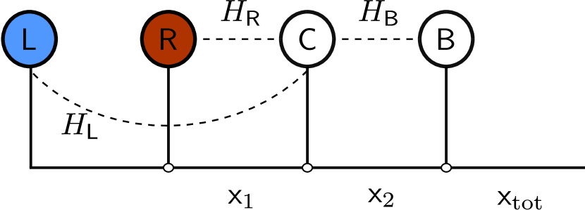
Figure 2: Graphical representation of the T-junction system as a fusion tree of the four anyons, corresponding to the basis choice made in the text, see Eq. (3). Different sequences of the fusion outcomes $\mathsf{x}_{1},\mathsf{x_{2}},\mathsf{x}_{\textrm{tot}}$ define the basis states of the Hilbert space. Three Hamiltonians $H_{\mathsf{L}},H_{\mathsf{R}},H_{\mathsf{B}}$ describe the interaction between different pairs of anyons. In particular, $H_{\mathsf{L}}$ couples the anyons $\mathsf{L}$ and $\mathsf{C}$ which, in this basis, are not nearest neighbors.

II.1 Ground state degeneracy

To prove that the Hamiltonian (2) is of any use for TQC, we must identify a degenerate manifold of its ground states, at least in some regions of the parameter space spanned by the energies $\epsilon_{i,\mathsf{K}}$.

It has been shown that tunneling couplings between anyons lift completely the topological degeneracy of the ground state bonderson09b , and the Hamiltonian (2) makes no exception if all $\epsilon_{\mathsf{a,K}}$ are non-zero. On the other hand, if all the couplings are zero, the ground state manifold coincides with the whole Hilbert space of the anyon system. We focus here on the intermediate domain between these two extreme cases, namely when only a subspace of the full Hilbert space has its degeneracy left intact.

The Hamiltonian (2) has an $n$-fold degenerate ground state when at least one of the $H_{\mathsf{K}}$ is zero and one is non-zero. Let us consider $H_{\mathsf{L}}=H_{\mathsf{R}}=0$, $\epsilon_{\mathsf{a,B}}>0$. The two anyons $\mathsf{L}$ and $\mathsf{R}$ are completely decoupled and share an arbitrary topological charge $\mathsf{x}_{1}$ which may assume one of the $n$ different values $\{\mathsf{f}_{i}\}$, while the anyons $\mathsf{B}$ and $\mathsf{C}$ fuse into the Abelian channel $\mathsf{a}$. The total topological charge equals $\mathsf{x}_{\textrm{tot}}=(\mathsf{t_{R}}\times\mathsf{t_{L}})\times(\mathsf{t_{B}}\times\mathsf{t_{C}})=\mathsf{x}_{1}\times\mathsf{a}$. Since $\mathsf{a}$ is Abelian, the fusion $\mathsf{x}_{1}\times\mathsf{a}$ can only have one possible outcome, and additionally there cannot be another charge $\mathsf{x}^{\prime}_{1}$ such that $\mathsf{x}^{\prime}_{1}\times\mathsf{a}$ has the same outcome. Therefore there exists a one-to-one mapping between the charges $\mathsf{x}_{1}$ and $\mathsf{x}_{\textrm{tot}}$, implying that the ground state wave function $|\Psi\rangle$ will generically be a superposition of $n$ orthogonal ground states $\Psi_{i}$ with total topological charge $\mathsf{f}_{i}\times\mathsf{a}$, $|\Psi\rangle=\sum_{i}a_{i}|\mathsf{f}_{i}\times\mathsf{a}\rangle$.

When a second coupling, say $H_{\mathsf{L}}$, is also nonzero, the anyon $\mathsf{L}$ fuses with $\mathsf{t_{C}}\times\mathsf{t_{B}}=\mathsf{a}$ and the three have a total charge $\mathsf{t}\times\mathsf{a}$. The overall degeneracy cannot change, since $\mathsf{t_{R}}\times(\mathsf{t_{L}}\times\mathsf{t_{B}}\times\mathsf{t_{C}})=\mathsf{t}\times(\mathsf{t}\times\mathsf{a})=(\sum_{i}\mathsf{f}_{i})\times\mathsf{a}$, which again gives $n$ orthogonal states.

We conclude that if all the couplings $H_{\mathsf{K}}$ are neither on nor off at the same time, the ground state of the Hamiltonian (2) has an $n$-fold degeneracy.

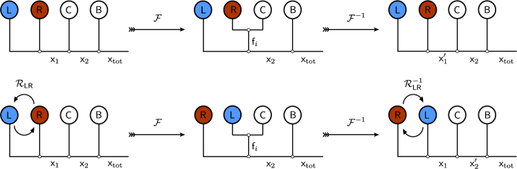
Figure 3: Top: graphical representation of Eq. (5). The fusion outcomes are explicitly written along the fusion tree. To write down the projectors $\Pi^{\mathsf{R}}_{i}$ in the basis of Fig. 3, we need two $\mathcal{F}$-moves. A similar transformation, not shown, is needed to write down $\Pi^{\mathsf{B}}_{i}$, see Eq. (4). Bottom: in the case of $\Pi^{\mathsf{L}}_{i}$, two braiding matrices $\mathcal{R}_{\mathsf{LR}}$ make their appearance in addition to the $\mathcal{F}$-moves. This introduces the braiding matrix $\mathcal{R}_{\mathsf{LR}}$ in the Hamiltonian of the $T$-junction.

II.2 Projectors

In order to describe the wave function evolution in the $n$-fold degenerate ground state subspace of (2), we need to write down the Hamiltonian (2) explicitly in a certain basis. To describe the evolution and the eigenstates of this system we closely follow the methods used for the study of anyon chains and lattices (see e.g. feiguin07 ; trebst08 ; gils09 ; ardonne11 ; ludwig11 ).

The different quantum states of a system of anyons can be specified by the sequence of fusion outcomes along a certain fusion path. The choice of a fusion path is equivalent to the choice of a basis in the Hilbert space. Once a fusion path is chosen, the projector of two anyons on a given channel $\mathsf{f}_{i}$ is represented by a simple diagonal matrix if the two anyons fuse directly together along the path with outcome $\mathsf{f}_{i}$. Otherwise a projector must be written via appropriate transformations called $\mathcal{F}$-matrices (see e.g. nayak08 ; preskill ; feiguin07 ). We choose the following fusion path shown also in Fig. 2:

$$\left(\left(\left(\mathsf{t_{L}}\times\mathsf{t_{R}}\to\mathsf{x}_{1}\right)\times\mathsf{t_{C}}\to\mathsf{x}_{2}\right)\times\mathsf{t_{B}}\to\mathsf{x}_{\textrm{tot}}\right),$$ (3)

with $\mathsf{x}_{1},\mathsf{x}_{2},\mathsf{x}_{\textrm{tot}}$ belonging to the sets of possible fusion channels at each step of the fusion path. All states in the Hilbert space can be written as $|\mathsf{x}_{1},\mathsf{x}_{2},\mathsf{x}_{\textrm{tot}}\rangle$. The basis (3) describes a path where $\mathsf{t_{L}}$ and $\mathsf{t_{R}}$ are first fused with outcome $\mathsf{x}_{1}$, then with $\mathsf{t_{C}}$ resulting in a second outcome $\mathsf{x}_{2}$, and finally with the fourth anyon $\mathsf{t_{B}}$ to give $\mathsf{x}_{\textrm{tot}}$. The latter is the total topological charge of the system: subspaces of the Hilbert space corresponding to different $\mathsf{x}_{\textrm{tot}}$ are decoupled. Adopting this basis we can now write down explicitly all the terms appearing in the Hamiltonian (2). To this purpose we consider different bases in which each operator has a diagonal form, and then we move to the basis in Eq. (3) using appropriate basis transformations.

We start with $\Pi^{\mathsf{B}}_{i}$. The anyons $\mathsf{t_{C}}$ and $\mathsf{t_{B}}$ are nearest neighbour, but they do not fuse directly together in our fusion path: to write $\Pi_{i}^{\mathsf{B}}$ we must use the appropriate $\mathcal{F}$-matrices,

$$\begin{split}\left[\Pi_{i}^{\mathsf{B}}(\mathsf{x_{1}},\mathsf{x}_{\textrm{tot}})\right]_{\mathsf{x}_{2}^{\prime},\mathsf{x}_{2}}&=\sum_{\mathsf{y}}\left(\mathcal{F}^{\mathsf{x}_{1}\mathsf{t_{C}t_{B}}}_{\mathsf{x}_{\textrm{tot}}}\right)^{-1}_{\mathsf{x}_{2}^{\prime},\mathsf{f}_{i}}\,\delta_{\mathsf{f}_{i},\mathsf{y}}\,\left(\mathcal{F}^{\mathsf{x}_{1}\mathsf{t_{C}t_{B}}}_{\mathsf{x}_{\textrm{tot}}}\right)_{\mathsf{y},\mathsf{x}_{2}}=\\ &=\left(\mathcal{F}^{\mathsf{x}_{1}\mathsf{t_{C}t_{B}}}_{\mathsf{x}_{\textrm{tot}}}\right)^{-1}_{\mathsf{x}_{2}^{\prime},\mathsf{f}_{i}}\left(\mathcal{F}^{\mathsf{x}_{1}\mathsf{t_{C}t_{B}}}_{\mathsf{x}_{\textrm{tot}}}\right)_{\mathsf{f}_{i},\mathsf{x}_{2}}\end{split}$$ (4)

with $\mathsf{y}\,\in\,\{\mathsf{f_{i}}\}$ and $\mathsf{x}_{2},\mathsf{x}^{\prime}_{2}$ belonging to the set of fusion channels of three $\mathsf{t}$ anyons. As indicated on the left hand side of Eq. (4), the matrix elements of the projector depend on indices $\mathsf{x_{1}},\mathsf{x}_{\textrm{tot}}$. In a similar way we obtain for $\Pi_{i}^{\mathsf{R}}$ the following form:

$$\left[\Pi^{\mathsf{R}}_{i}(\mathsf{x_{2}})\right]_{\mathsf{x}_{1}^{\prime},\mathsf{x}_{1}}=\left(\mathcal{F}^{\mathsf{t_{L}t_{R}t_{C}}}_{\mathsf{x}_{2}}\right)^{-1}_{\mathsf{x}_{1}^{\prime},\mathsf{f}_{i}}\left(\mathcal{F}^{\mathsf{t_{L}t_{R}t_{C}}}_{\mathsf{x_{2}}}\right)_{\mathsf{f}_{i},\mathsf{x}_{1}}$$ (5)

with $\mathsf{x}_{1},\mathsf{x}^{\prime}_{1}\;\in\;\{\mathsf{f}_{i}\}$. The graphical representation of this equation is shown in the top panel of Fig. 3.

Unlike the two other cases, in the fusion tree of Fig. 2 the anyons $\mathsf{L}$ and $\mathsf{C}$ are not nearest neighbours in the chosen basis. Since they would be nearest neighbors if $\mathsf{L}$ and $\mathsf{R}$ were interchanged, the transformation to a basis when they fuse directly together includes a braiding matrix $\mathcal{R}_{\mathsf{LR}}$, as shown in the bottom panel of Fig. 3. The particular braiding matrix ($\mathcal{R}_{\mathsf{LR}}$ or $\mathcal{R}^{-1}_{\mathsf{LR}}$) that appears in this basis transformation depends on the real space positions of the anyons and on the microscopic details of the Hamiltonian. The two possible choices correspond to two mirror-symmetric anyon models bondersonthesis . It is this term that is responsible for the appearance of braiding during the adiabatic Hamiltonian evolution. In particular mirroring the T-junction layout inverts the chirality of $\mathcal{R}$. As shown in the bottom panel of Fig. 3, the projector $\Pi^{\mathsf{L}}_{i}$ can be obtained from $\Pi_{i}^{\mathsf{R}}$ via $\mathcal{R}_{\mathsf{LR}}$

$$\mathcal{R}_{\mathsf{LR}}^{-1}\,\Pi^{\mathsf{R}}_{i}\mathcal{R}_{\mathsf{LR}}=\Pi^{\mathsf{L}}_{i}$$ (6)

In the fusion basis (3), $\mathcal{R}_{\mathsf{LR}}$ is a diagonal matrix and, explicitly, we have

$$\begin{split}\left[\Pi^{\mathsf{L}}_{i}(\mathsf{x_{2}})\right]_{\mathsf{x}_{1}^{\prime},\mathsf{x}_{1}}&=\left(\mathcal{R}_{\mathsf{LR}}^{-1}\right)_{\mathsf{x}^{\prime}_{1}}\left(\Pi^{\mathsf{R}}_{i}\right)_{\mathsf{x}_{1}^{\prime},\mathsf{x}_{1}}\left(\mathcal{R}_{\mathsf{LR}}\right)_{\mathsf{x}_{1}}=\\ &=\left(\mathcal{R}_{\mathsf{LR}}^{-1}\right)_{\mathsf{x}_{1}^{\prime}}\left(\mathcal{F}^{\mathsf{t_{L}t_{R}t_{C}}}_{\mathsf{x}_{2}}\right)^{-1}_{\mathsf{x}_{1}^{\prime},\mathsf{f}_{i}}\left(\mathcal{F}^{\mathsf{t_{L}t_{R}t_{C}}}_{\mathsf{x}_{2}}\right)_{\mathsf{f}_{i},\mathsf{x}_{1}}\left(\mathcal{R}_{\mathsf{LR}}\right)_{\mathsf{x}_{1}}.\end{split}$$ (7)

Knowing the $\mathcal{F}$-matrices of a given anyon model, Eqs. (4,5,7) allow to write explicitly the four-anyon Hamiltonian (2). In particular, we note that the braiding operator $\mathcal{R}_{\mathsf{LR}}$ now appears explicitly in

$$H_{\mathsf{L}}=\sum_{i}\epsilon_{i,\mathsf{L}}\,\Pi^{\mathsf{L}}_{i}=\sum_{i}\epsilon_{i,\mathsf{L}}\,\mathcal{R}^{-1}_{\mathsf{LR}}\,\Pi^{\mathsf{R}}_{i}\,\mathcal{R}_{\mathsf{LR}}.$$ (8)

Before concluding this section, we point out that because the interactions are local, the fusion product $\mathsf{t_{B}}\times\mathsf{t_{C}}$ cannot be affected by the braiding of $R$ and $L$. The projectors $\Pi_{i}^{\mathsf{B}}$ and the braiding operator $\mathcal{R}_{\mathsf{LR}}$ must therefore commute:

$$\Pi_{i}^{\mathsf{B}}\mathcal{R}_{\mathsf{LR}}=\mathcal{R}_{\mathsf{LR}}\,\Pi_{i}^{\mathsf{B}}.$$ (9)

III The adiabatic cycle

In this section we show that the braiding of the anyons $\mathsf{R}$ and $\mathsf{L}$ appears as a result of any closed path in parameter space starting from a point where only $H_{\mathsf{B}}\neq 0$, and continuously passing through the points where first only $H_{\mathsf{L}}\neq 0$, and finally only $H_{\mathsf{R}}\neq 0$ in such a way that the degeneracy is always preserved. For the ease of presentation we divide the path into three separate steps of duration $T$ such that during each step one of $H_{\mathsf{K}}$ is turned on and one off. The time evolution of the Hamiltonian along such a path is shown in Fig. 4.

Let us consider the evolution of the ground state wave function $|\Psi(t)\rangle$ of $H$ along this adiabatic cycle. The wave function can at any moment be written as a superposition over states with different total topological charge $\mathsf{x}_{\textrm{tot}}$,

$$|\Psi(t)\rangle=\sum_{\mathsf{x}_{\textrm{tot}}}\,a_{\mathsf{x}_{\textrm{tot}}}\,|\Psi_{\mathsf{x}_{\textrm{tot}}}(t)\rangle.$$ (10)

The states $|\Psi_{\mathsf{x}_{\textrm{tot}}}(t)\rangle$ define the $n$-fold ground state manifold. The absolute values of the superposition coefficients $a_{\mathsf{x}_{\textrm{tot}}}$ are conserved because the total topological charge is a conserved quantity. This implies that the time evolution of the ground state manifold is a diagonal operator in the basis given by $|\Psi_{\mathsf{x}_{\textrm{tot}}}(t)\rangle$. Therefore, each term in the superposition (10) can only acquire a phase, possibly dependent on $\mathsf{x}_{\textrm{tot}}$, or in other words the Berry matrix is diagonal in this basis. This allows us to follow the evolution of each $|\Psi_{\mathsf{x}_{\textrm{tot}}}(t)\rangle$ independently from all other states.

We should note that the superposition (10) is only possible if other anyons are present in the system other than $\mathsf{L},\mathsf{R},\mathsf{C},\mathsf{B}$. We imagine that these anyons do not interact with the T-junction while the adiabatic cycle is performed, so that their presence can be ignored.

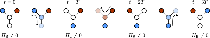
Figure 4: Illustration of the adiabatic cycle which reproduces the braiding operator $\mathcal{R}_{\mathsf{LR}}$ of two topological charges $\mathsf{t}$ (red and blue circles) in a four anyon system. The cycle is divided in three steps of duration $T$. At the end of each step only one interaction $H_{\mathsf{K}}$ is on. The arrows follow the transfer of an unpaired topological charge $\mathsf{t}$ at intermediate stages, represented as the spreading of the colored circles over different anyons.

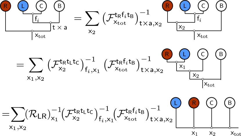
Figure 5: The derivation of Eq. (12). We transform the ground states $|\Psi_{\mathsf{x}_{\textrm{tot}}}(t)\rangle$ from the basis $\left((\mathsf{t_{L}}\times\mathsf{t_{C}}\to\mathsf{f}_{i})\times\sf{t_{B}}\to\sf{t}\times\sf{a}\right)$ to the basis (3). The phase factor $\left(\mathcal{F}^{\mathsf{t}\mathsf{a}\mathsf{t}}_{\mathsf{x}_{\textrm{tot}}}\right)_{\mathsf{t}\times\mathsf{a},\mathsf{t}\times\mathsf{a}}$ from Eq. (12) is not explicitly shown here.

During the first step $0\leq t\leq T$, the anyon $\mathsf{R}$ is left unpaired from the other three. The topological charge of the three anyons $\mathsf{L,C,B}$ is then conserved and equal to its initial value $\mathsf{t_{L}}\times(\mathsf{t_{C}}\times\mathsf{t_{B}})=\mathsf{t}\times\mathsf{a}$. The general form of a wave function satisfying this constraint is given by:

$$|\Psi_{\mathsf{x}_{\textrm{tot}}}(t)\rangle=\sum_{\mathsf{x}_{1},\mathsf{x}_{2},\mathsf{f}_{i}}\,U_{\mathsf{x}_{\textrm{tot}},\mathsf{x}_{1},\mathsf{x}_{2},\mathsf{f}_{i}}\,\alpha_{\mathsf{f}_{i}}(t)\,|\mathsf{x_{1}},{\mathsf{x}_{2},\mathsf{x}_{\textrm{tot}}}\rangle,$$ (11)

where $\alpha_{\mathsf{f}_{i}}(t)$ can always be chosen to not depend on $\mathsf{x}_{\textrm{tot}}$, and the unitary matrix $U$ is the transformation from the basis $\left((\mathsf{t_{L}}\times\mathsf{t_{C}}\to\mathsf{f}_{i})\times\sf{t_{B}}\to\sf{t}\times\sf{a}\right)$, where the anyons L, C and B fuse directly into $\mathsf{t}\times\mathsf{a}$ before adding the anyon R, to the basis (3):

$$U_{\mathsf{x}_{\textrm{tot}},\mathsf{x}_{1},\mathsf{x}_{2},\mathsf{f}_{i}}=\left(\mathcal{F}^{\mathsf{t}\mathsf{a}\mathsf{t}}_{\mathsf{x}_{\textrm{tot}}}\right)_{\mathsf{t}\times\mathsf{a},\mathsf{t}\times\mathsf{a}}\left(\mathcal{R}_{\mathsf{LR}}^{-1}\right)_{\mathsf{x}_{1}}\\ \times\left(\mathcal{F}^{\sf{t_{R}t_{L}t_{C}}}_{\mathsf{x}_{2}}\right)_{\mathsf{f}_{i},\mathsf{x}_{1}}^{-1}\left(\mathcal{F}^{\sf{t_{R}}\mathsf{f}_{i}\sf{t_{B}}}_{\mathsf{x}_{\textrm{tot}}}\right)_{\sf{t}\times\sf{a},\mathsf{x}_{2}}^{-1}.$$ (12)

The $\mathcal{F}$- and $\mathcal{R}$-moves required for this transformation are shown in Fig. 5.

In particular, at $t=0$, only $H_{\mathsf{B}}\neq 0$ and each $|\Psi_{\mathsf{x}_{\textrm{tot}}}(0)\rangle$ is an eigenstate of $\Pi^{\mathsf{B}}_{\mathsf{a}}$ defined in Eq. (4):

$$|\Psi_{\mathsf{x_{\textrm{tot}}}}(0)\rangle=\left(\mathcal{F}^{\mathsf{t}\mathsf{a}\mathsf{t}}_{\mathsf{x}_{\textrm{tot}}}\right)_{\mathsf{t}\times\mathsf{a},\mathsf{t}\times\mathsf{a}}\sum_{\mathsf{x}_{1},\mathsf{x}_{2}}\left(\mathcal{R}_{\mathsf{LR}}^{-1}\right)_{\mathsf{x}_{1}}\\ \times\left(\mathcal{F}^{\mathsf{x}_{1}\mathsf{t_{C}t_{B}}}_{\mathsf{x}_{\textrm{tot}}}\right)^{-1}_{\mathsf{a},\mathsf{x}_{2}}\left(\mathcal{F}^{\mathsf{t_{R}}\mathsf{t_{L}a}}_{\mathsf{x}_{\textrm{tot}}}\right)^{-1}_{\mathsf{t\times a},\mathsf{x}_{1}}|\mathsf{x}_{1},\mathsf{x}_{2},\mathsf{x}_{\textrm{tot}}\rangle\,,$$ (13)

These wavefunctions (13) can be obtained from the Eqs. (11) and (12) by substituting $\alpha_{\mathsf{f}_{i}}(0)=\left(\mathcal{F}^{\sf t_{L}t_{C}t_{B}}_{\sf t\times a}\right)^{-1}_{\sf a,f_{i}}$ and applying the pentagon equation bondersonthesis ; preskill . The presence of the last $\mathcal{F}$ symbol in Eq. (13) implies $\mathsf{x}_{1}=\mathsf{x}_{\textrm{tot}}\times\mathsf{a}$, which simplifies the sum over $\mathsf{x_{1}}$ due to $\mathsf{a}$ being Abelian. The phase factor $(\mathcal{R}_{\mathsf{LR}}^{-1})_{\mathsf{x}_{1}}$ is needed in order to guarantee the independence of $\alpha_{\mathsf{f}_{i}}(t)$ on $\mathsf{x}_{\textrm{tot}}$.

As $t$ evolves from $0$ to $T$, these states acquire a Berry phase,

$$\theta_{T} =\int_{0}^{T}\langle\Psi_{\mathsf{x}_{\textrm{tot}}}(t)|\,\partial_{t}|\Psi_{\mathsf{x}_{\textrm{tot}}}(t)\rangle\operatorname{d\!}t=$$

$$=\int_{0}^{T}\sum_{\mathsf{f}_{i}}\alpha^{*}_{\mathsf{f}_{i}}\partial_{t}\alpha_{\mathsf{f}_{i}}\operatorname{d\!}t.$$ (14)

The time-independent unitary matrix $U$ naturally drops out of the expression for the Berry phase. We conclude that the Berry phase acquired in our basis during the first step is the same for every state, or in other words it is Abelian.

At $t=T$, only $H_{\mathsf{L}}\neq 0$, and the ground state wave function must be in an eigenstate of $\Pi^{\mathsf{L}}_{\mathsf{a}}$,

$$|\Psi_{\mathsf{x}_{\textrm{tot}}}(T)\rangle=\sum_{\mathsf{x}_{1}}\left(\mathcal{F}^{\mathsf{{t_{R}t_{L}t_{C}}}}_{\mathsf{x}_{2}}\right)^{-1}_{\mathsf{a},\mathsf{x}_{1}}\left(\mathcal{R}_{\mathsf{LR}}^{-1}\right)_{\mathsf{x}_{1}}|\mathsf{x}_{1},\mathsf{x}_{2},\mathsf{x}_{\textrm{tot}}\rangle,$$ (15)

now with $\mathsf{x}_{2}=\mathsf{t}\times\mathsf{a}$ since $\mathsf{L}$ and $\mathsf{C}$ fuse into $\mathsf{a}$, and the phases once again fixed by the requirement that $\alpha_{\mathsf{f}_{i}}$ do not depend on $\mathsf{x}_{\textrm{tot}}$. Note that the wave functions (15) are of form given by Eq. (11). The net result of the evolution from $t=0$ to $t=T$ is the transfer from $\mathsf{L}$ to $\mathsf{B}$ of an unpaired topological charge $\mathsf{t}$.

During the second step $T\leq t\leq 2T$ the wave function coefficients can be chosen to be independent on $\mathsf{x}_{\textrm{tot}}$ in the basis of Eq. (3). The wave function evolves from the eigenstate (15) of $\Pi^{\mathsf{L}}_{\mathsf{a}}$ into an eigenstate of $\Pi^{\mathsf{R}}_{\mathsf{a}}$. Due to the relation (6) and Eq. (15) we can write the ground state wave functions at $t=2T$ as

$$|\Psi_{\mathsf{x}_{\textrm{tot}}}(2T)\rangle=\sum_{\mathsf{x}_{1}}\left(\mathcal{F}^{\mathsf{{t_{L}t_{R}t_{C}}}}_{\mathsf{x}_{2}}\right)^{-1}_{\mathsf{a},\mathsf{x}_{1}}|\mathsf{x}_{1},\mathsf{x}_{2},\mathsf{x}_{\textrm{tot}}\rangle.$$ (16)

The integral of the Berry connection $\langle\Psi_{\mathsf{x}_{\textrm{tot}}}(t)|\,\partial_{t}|\Psi_{\mathsf{x}_{\textrm{tot}}}(t)\rangle$ from $T$ to $2T$ is common to all states and provides an Abelian Berry phase due to the independence of all the coefficients on $\mathsf{x}_{\textrm{tot}}$.

In the last step, $2T\leq t\leq 3T$, we repeat the procedure of the first one. We write the wave function in a basis $\left((\mathsf{t_{R}}\times\mathsf{t_{C}}\to\mathsf{f}_{i})\times\sf{t_{B}}\to\sf{t}\times\sf{a}\right)$, where $\mathsf{t_{R}},\mathsf{t_{C}},\mathsf{t_{B}}$ fuse into $\mathsf{t}\times\mathsf{a}$ before the anyon $\mathsf{L}$ is added. The corresponding transformation to the basis (3) is given by the Eq. (12), but without the matrix $\left(\mathcal{R}_{\mathsf{LR}}\right)^{-1}$. This ensures that the wave function $|\Psi_{\mathsf{x}_{\textrm{tot}}}(t)\rangle$ stays continuous at $t=2T$. In this last step, the wave function acquires another Abelian Berry phase and ends up again in an eigenstate of $\Pi^{\mathsf{B}}_{\mathsf{a}}$. We end up with:

$$|\Psi_{\mathsf{x_{\textrm{tot}}}}(3T)\rangle=\left(\mathcal{F}^{\mathsf{t}\mathsf{a}\mathsf{t}}_{\mathsf{x}_{\textrm{tot}}}\right)_{\mathsf{t}\times\mathsf{a},\mathsf{t}\times\mathsf{a}}\sum_{\mathsf{x}_{1},\mathsf{x}_{2}}\left(\mathcal{F}^{\mathsf{x}_{1}\mathsf{t_{C}t_{B}}}_{\mathsf{x}_{\textrm{tot}}}\right)^{-1}_{\mathsf{a},\mathsf{x}_{2}}\\ \times\left(\mathcal{F}^{\mathsf{t_{R}}\mathsf{t_{L}a}}_{\mathsf{x}_{\textrm{tot}}}\right)^{-1}_{\mathsf{t\times a},\mathsf{x}_{1}}|\mathsf{x}_{1},\mathsf{x}_{2},\mathsf{x}_{\textrm{tot}}\rangle.$$ (17)

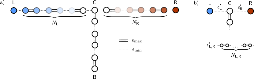
Figure 6: Panel (a): three staggered anyon chains forming a T-junction. Weak ($\epsilon_{\textrm{min}}$, dashed lines) and strong ($\epsilon_{\textrm{max}}$, double solid lines) couplings alternate. The bottom arm of the T-junction, connecting the original anyons $\mathsf{C}$ and $\mathsf{B}$, is in a dimerized phase with no unpaired anyons and approximately contains no net topological charge. On the other hand, in the right and left arm the dimerization leaves two almost unpaired anyons $\mathsf{L}$ and $\mathsf{R}$ at the end (blue and red dot). Due to the residual coupling, the topological charge of $\mathsf{L}$ and $\mathsf{R}$ is spread over the neighboring anyon pairs, as represented by the color gradings. The left and right arm are in therefore in the non-trivial phase. The two arms interact weakly via the centre of the T-junction, leading to renormalized couplings $\epsilon^{\prime}_{\mathsf{L}}$ and $\epsilon^{\prime}_{\mathsf{R}}$ between $\mathsf{L}$, $\mathsf{R}$ and $\mathsf{C}$, as in panel (b). The residual interaction splits the ground state degeneracy of an energy exponentialy small in the length of the chains.

Having performed an adiabatic evolution over a closed path, the final wave function must be connected to the initial one via a unitary matrix $\mathcal{U}$, $|\Psi(3T)\rangle=\mathcal{U}|\Psi(0)\rangle$. Using Eq. (13) and (17) we find

$$\langle\Psi_{\mathsf{x}_{\textrm{tot}}}(0)|\Psi_{\mathsf{x}_{\textrm{tot}}}(3T)\rangle=(\mathcal{R}_{LR})_{\mathsf{x}_{1}}$$ (18)

where we recall that $\mathsf{x}_{\textrm{tot}}=\mathsf{x}_{1}\times\mathsf{a}$. For the whole wave function we can write

$$|\Psi(3T)\rangle=\mathcal{R}_{\mathsf{LR}}\,|\Psi(0)\rangle$$ (19)

up to an Abelian Berry phase. This means that the braiding of anyons $\mathsf{L}$ and $\mathsf{R}$ was performed in the adiabatic cycle. By performing the whole protocol in reverse, we obtain instead the inverse braiding.

IV Discussion and conclusions

IV.1 Restoring scalability and topological protection

The braiding procedure of Sec. III relies on the ability to turn off the pairwise interactions $H_{\textsf{K}}$ completely. This is only possible if the separation between the anyons becomes infinite, and hence one may argue that this procedure is only approximating topological quantum computation. In a finite system the non-Abelian Berry phase will in general have a correction, and additionally non-adiabatic errors will appear due to the presence of finite ground state splitting dassarma11 .

This imperfection can be removed and the topological nature of the braiding can be restored by bringing the anyons $\mathsf{L},\mathsf{R},\mathsf{B}$ further away from the central one $\mathsf{C}$. If anyonic chains with controllable couplings are then introduced along the three arms of the T-junction (see Fig. 6), this still allows to perform the braiding in a similar fashion, but with a higher fidelity. Since we are interested in the low energy spectrum of the Hamiltonian we approximate the interactions between nearest-neighbor anyons $\mathsf{K},\mathsf{K^{\prime}}$ with the projector $\Pi_{\mathsf{a}}^{\mathsf{K,K^{\prime}}}$ over their lowest energy topological charge and we consider all the other fusion channels to have the same energy, so that the Hamiltonian of each junction becomes:

$$H_{\mathsf{K,K^{\prime}}}=-\epsilon\Pi_{\mathsf{a}}^{\mathsf{K,K^{\prime}}},$$ (20)

where $\mathsf{a}$ should again be Abelian. We require that $\epsilon$ can be varied in a range $(\epsilon_{\textrm{min}},\epsilon_{\textrm{max}})$, so that the chains can be driven into a staggered phase with alternating weak and strong couplings, as in the Kitaev Majorana chain Kit01 and its parafermionic generalization fendley12 .

The termination of the chain ending with a weak link differs from the termination by a strong link by the presence of an extra $\mathsf{t}$ anyon, and the chain ending with a strong link can be continuously connected to a chain of fully fused $\mathsf{a}$-type anyons. This means that if the chain is gapped, whenever it ends in a weak link, its end has a topological charge of $\mathsf{t}$, spread over several anyons, as shown in Fig. 6. While we are not aware of a proof that a general anyonic chain with staggered antiferromagnetic couplings is gapped, it is true for many relevant cases gils09 ; fid08 ; lau12 . When $\epsilon_{\textrm{min}}\ll\epsilon_{\textrm{max}}$, the effective minimal coupling between an unpaired anyon at the edge of the T-junction and the central anyon $\mathsf{C}$ can be calculated perturbatively, and it is equal to $\epsilon^{\prime}\simeq\epsilon_{\textrm{min}}(\kappa\epsilon_{\textrm{min}}/\epsilon_{\textrm{max}})^{N}$, with $N$ the number of anyon pairs in the chain, and $\kappa$ a geometric factor which depends on the specific anyon model. For Ising anyons $\kappa=1$, and for Fibonacci anyons $\kappa=2/\phi^{2}$, with $\phi=\left(1+\sqrt{5}\right)/2$ the golden ratio fid08 ; lau12 . The maximal coupling is achieved in the staggered configuration which ends with a strong bond, and the maximal coupling $\epsilon_{\textrm{max}}$ is only weakly modified.

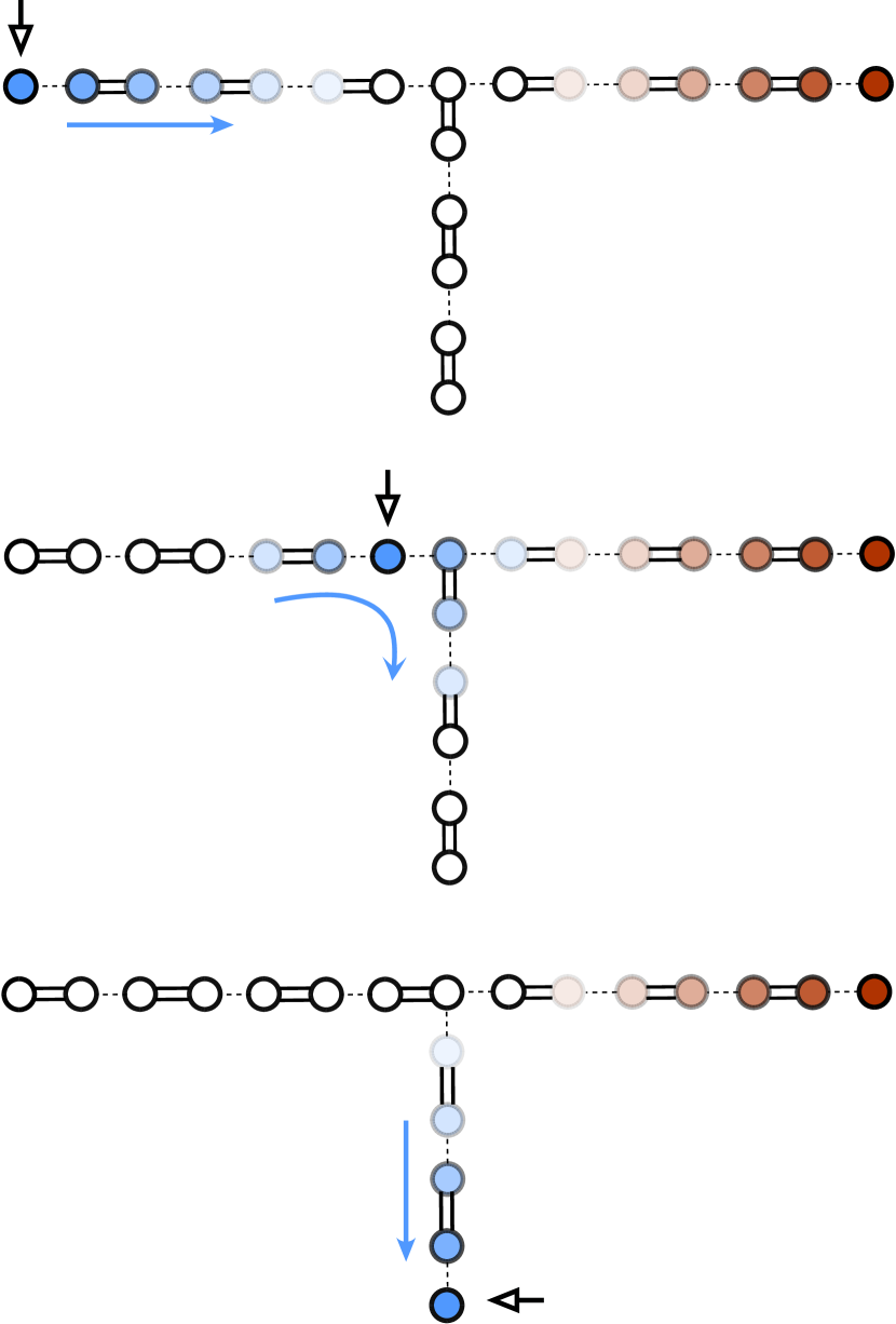
Figure 7: The first step of the adiabatic braiding sequence realized in a system of staggered anyonic chains. The topological charge $\mathsf{t}$ is moved from the left arm of the junction to the bottom arm. As in Fig. 6, blue and red colors represent a topological charge $\mathsf{t}$ spread over several anyons. The charges are localized at domain walls between the two possible phases of the staggered chain. Domain walls can be moved: each movement involves three different anyons of the chain. The domain wall that is moved is marked by a black arrow.

To implement the braiding, each part of the adiabatic evolution can be decomposed into steps which require to change the pairwise couplings of three anyons, just as it happens for the steps illustrated in Fig. 4. In this way, during the adiabatic cycle, we create and move domain walls which drive the transition between the two different staggered configurations of the chains (see Fig. 7). The two unpaired topological charges encoding the computational degree of freedom are localized in these domain walls which are moved along the three arms. Since the distance between the unpaired charges is always larger than the length $N$ of a single arm of the T-junction, their residual interaction is exponentially suppressed, allowing to likewise exponentially suppress the error in the final result.

IV.2 Summary

In summary, we have investigated an approach to topological quantum computation. In order to implement the necessary braiding operations of non-Abelian anyons, we couple the anyons instead of moving them or measuring their state. We have considered a simple system composed of four interacting non-Abelian anyons in a T-junction geometry and we have shown how adiabatic control over the interactions results in the Berry matrix expected when two anyons are moved around each other. If the coupling between the anyons cannot be completely turned off, errors are introduced in the braiding operations due to the residual splitting of the ground state degeneracy. We have discussed how these errors can be limited by means of enlarging the number of anyons involved in the adiabatic evolution. The protection is exponential in the number of anyons which are added to the system, so the whole procedure is similar to increasing the separation between anyons in the original approach.

Our approach, inspired by recent theoretical proposals for the braiding of Majorana fermions in superconductors, is applicable to most anyon models. These include all the SU$(2)_{k}$ models (such as the Ising and Fibonacci anyons expected to appear in fractional quantum Hall systems), as well as the fractionalized Majorana fermions very recently proposed in Refs. cla12 ; lin12 ; cheng12 ; vaezi12 ; wen12 ; fendley12 .

A possible implementation of our scheme in the fractional quantum Hall systems, would require to engineer systems of dots hosting single anyonic quasiparticles and to tune their interactions via the voltages induced by gates or scanning tips, in a similar spirit to the blockade measurement of topological charge vanheck12 .

Alternative, but even more exotic, implementations of this scheme include for example the braiding procedure presented in Refs. lin12 ; barkeshli12 for fractional Majorana fermions in superconductor/quantum-Hall heterostructures. Additionally, the recent progress in the design of several systems thought to host non-Abelian excitations, ranging from physical realizations of the Kitaev honeycomb lattice model kitaev06 (see, for example duan03 ; zoller06 ; jackeli09 ) to ultracold atomic gases subjected to artificial gauge potentials cooper08 ; lewensteinbook , could also fall into the category of systems where interactions between anyons are easier to control than their positions.

References

- (1) A. Y. Kitaev, Ann. Phys. 303, 2-30 (2003).
- (2) C. Nayak, S. H. Simon, A. Stern, M. Freedman and S. Das Sarma, Rev. Mod. Phys. 80, 1083 (2008).
- (3) P. Bonderson, M. Freedman, and C. Nayak, Phys. Rev. Lett. 101, 010501 (2008).
- (4) P. Bonderson, M. Freedman, and C. Nayak, Ann. Phys. 324, 787 (2009).
- (5) E. Fradkin, C. Nayak, A. Tsvelik and F. Wilczek, Nucl. Phys. B 516 704-718 (1998).
- (6) S. Das Sarma, M. Freedman, and C. Nayak, Phys. Rev. Lett. 94, 166802 (2005).
- (7) A. Stern and B. I. Halperin, Phys. Rev. Lett. 96, 016802 (2006).
- (8) P. Bonderson, A. Kitaev and K. Shtengel, Phys. Rev. Lett. 96, 016803 (2006).
- (9) P. Bonderson, K. Shtengel and J. K. Slingerland, Ann. Phys. 323, 2709-2755 (2008).
- (10) W. Bishara, P. Bonderson, C. Nayak, K. Shtengel and J. K. Slingerland, Phys. Rev. B 80, 155303 (2009).
- (11) R. L. Willett, L. N. Pfeiffer and K. W. West, PNAS 106, 8853 (2009)
- (12) R. L. Willett, L. N. Pfeiffer and K. W. West, Phys. Rev. B 82, 205301 (2010).
- (13) S. An, P. Jiang, H. Choi, W. Kang, S. H. Simon, L. N. Pfeiffer, K. W. West and K. W. Baldwin, arXiv:1112.3400 (2011).
- (14) R. L. Willett, L. N. Pfeiffer and K. W. West, arXiv:1204.1993 (2012).
- (15) B. J. Overbosch and X.-G. Wen, arXiv:0706.4339.
- (16) W. Bishara and C. Nayak, Phys. Rev. B 80, 155304 (2009).
- (17) B. Rosenow, B. I. Halperin, S. H. Simon and A. Stern, Phys. Rev. Lett. 100, 226803 (2008).
- (18) B. Rosenow and S. H. Simon, Phys. Rev. B 85, 201302(R) (2012).
- (19) D. J. Clarke and K. Shtengel, New J. Phys. 13, 055005 (2011).
- (20) A. Y. Kitaev, Phys. Usp. 44, 131 (2001).
- (21) R. M. Lutchyn, J. D. Sau, and S. Das Sarma, Phys. Rev. Lett. 105, 077001 (2010).
- (22) Y. Oreg, G. Refael, and F. von Oppen, Phys. Rev. Lett. 105, 177002 (2010).
- (23) J. Alicea, Y. Oreg, G. Refael, F. von Oppen, and M. P. A. Fisher, Nature Phys. 7, 412 (2011).
- (24) J. D. Sau, D. J. Clarke, and S. Tewari, Phys. Rev. B 84, 094505 (2011).
- (25) B. van Heck, A. R. Akhmerov, F. Hassler, M. Burrello and C. W. J. Beenakker, New J. Phys. 14, 035019 (2012).
- (26) B. I. Halperin, Y. Oreg, A. Stern, G. Refael, J. Alicea and F. von Oppen, Phys. Rev. B 85, 144501 (2012).
- (27) A. Y. Kitaev, Ann. Phys. 321, 2 (2006).
- (28) P. Bonderson, PhD Thesis, California Institute of Technology (2007).
- (29) J. Preskill, Lecture Notes on Topological Quantum Computation, available online at www.theory.caltech.edu/preskill/ph219/topological.pdf.
-
(30)
In the general case, the interactions between and the other anyons may favor different Abelian fusion channels if all the fusions assume the same topological charge.
The main example is the case of Ising anyons , which obey the fusion rules , , with both and Abelian; in this case changing the favored fusion channel of the pairwise interaction between (or ) and determines a change in the chirality of the braiding Sau11 ; hal12 . This is due to an additional symmetry of the Ising anyon model:
where is the projector over the fermionic fusion channel . This relation implies that changing the favored fusion channel for one of the two anyons or , the role of and are exchanged throughout the adiabatic cycle and effectively reverses the braiding direction.(21) - (31) P. Bonderson, Phys. Rev. Lett. 103, 110403 (2009).
- (32) A. Feiguin, S. Trebst, A. W. W. Ludwig, M. Troyer, A. Y. Kitaev, Z. Wang, and M. H. Freedman, Phys. Rev. Lett. 98, 160409 (2007).
- (33) S. Trebst, E. Ardonne, A. Feiguin, D. A. Huse, A. W. W. Ludwig and M. Troyer, Phys. Rev. Lett. 101, 050401 (2008).
- (34) C. Gils, E. Ardonne, S. Trebst, A. W. W. Ludwig, M. Troyer, and Z. Wang, Phys. Rev. Lett. 103, 070401 (2009).
- (35) E. Ardonne, J. Gukelberger, A. W. W. Ludwig, S. Trebst and M. Troyer, New J. Phys. 13, 045006 (2011).
- (36) D. Poilblanc, A. W. W. Ludwig, S. Trebst, and M. Troyer, Phys. Rev. B 83, 134439 (2011).
- (37) M. Cheng, V. Galitski, and S. Das Sarma, Phys. Rev. B 84, 104529 (2011).
- (38) P. Fendley, arXiv:1209.0472 (2012).
- (39) L. Fidkowski, G. Refael, N. E. Bonesteel and J. E. Moore, Phys. Rev. B 78, 224204 (2008).
- (40) C.R. Laumann, D.A. Huse, A.W.W. Ludwig, G. Refael, S. Trebst and M. Troyer, Phys. Rev. B 85, 224201 (2012).
- (41) D. J. Clarke, J. Alicea and K. Shtengel, Nat. Commun. 4, 1348 (2013).
- (42) N. H. Lindner, E. Berg, G. Refael, A. Stern, Phys. Rev. X 2, 041002 (2012).
- (43) M. Cheng, Phys. Rev. B 86, 195126 (2012).
- (44) A. Vaezi, Phys. Rev. B 87, 035132 (2013).
- (45) Y.-Z. You, C.-M. Jian, and X.-G. Wen, Phys. Rev. B 87, 045106 (2013).
- (46) B. van Heck, M. Burrello, A. Yacoby, and A. R. Akhmerov, Phys. Rev. Lett. 110, 086803 (2013).
- (47) M. Barkeshli, C.-M. Jian, and X.-L. Qi, Phys. Rev. B 87, 045130 (2013).
- (48) L.-M. Duan, E. Demler, and M. D. Lukin, Phys. Rev. Lett. 91, 090402 (2003).
- (49) A. Micheli, G. K. Brennen, and P. Zoller, Nature Phys. 2, 341 (2006).
- (50) G. Jackeli, and G. Khaliullin, Phys. Rev. Lett. 102, 017205 (2009).
- (51) N. R. Cooper, Adv. Phys. 57, 539 (2008).
- (52) M. Lewenstein, A. Sanpera and V. Ahufinger, Ultracold Atoms in Optical Lattices: Simulating quantum many-body systems, Oxford University Press (2012), Chap. 11 and references therein.