Cross-correlating cosmic IR and X-ray background fluctuations: evidence of significant black hole populations among the CIB sources

Abstract

In order to understand the nature of the sources producing the recently uncovered CIB fluctuations, we study cross-correlations between the fluctuations in the source-subtracted Cosmic Infrared Background (CIB) from Spitzer/IRAC data and the unresolved Cosmic X-ray Background (CXB) from deep Chandra observations. Our study uses data from the EGS/AEGIS field, where both datasets cover an $\simeq 8^{\prime}\times 45^{\prime}$ region of the sky. Our measurement is the cross-power spectrum between the IR and X-ray data. The cross-power signal between the IRAC maps at 3.6$\mu$m and 4.5$\mu$m and the Chandra [0.5-2] keV data has been detected, at angular scales ${{}_{>}\atop{}^{\sim}}20{{}^{\prime\prime}}$, with an overall significance of $\simeq 3.8\sigma$ and $\simeq 5.6\sigma$, respectively. At the same time we find no evidence of significant cross-correlations at the harder Chandra bands. The cross-correlation signal is produced by individual IR sources with 3.6$\mu$m and 4.5$\mu$m magnitudes $m_{AB}{{}_{>}\atop{}^{\sim}}$ 25-26 and [0.5-2] keV X-ray fluxes $\ll 7\times 10^{-17}$ $\rm erg/cm^{2}/s\$. We determine that at least $15-25\%$ of the large scale power of the CIB fluctuations is correlated with the spatial power spectrum of the X-ray fluctuations. If this correlation is attributed to emission from accretion processes at both IR and X-ray wavelengths, this implies a much higher fraction of accreting black holes than among the known populations. We discuss the various possible origins for the cross-power signal and show that neither local foregrounds, nor the known remaining normal galaxies and active galactic nuclei (AGN) can reproduce the measurements. These observational results are an important new constraint on theoretical modeling of the near-IR CIB fluctuations.

1 Introduction

Cosmic backgrounds contain emissions produced during the entire history of the Universe including from objects individually inaccessible to telescopic studies. In different spectral regimes, the cosmic background probes different sources according to their emission mechanisms. Thus, cosmic X-ray background (CXB, $\sim$[0.5-10] keV) probes both emissions by accreting black holes (BHs) and thermal X-ray emission from hot ionized gas, such as in galaxy clusters. Whereas the cosmic infrared background (CIB) at the near-IR wavelengths (1-5$\mu$m) is sensitive to stellar emissions (see review by Kashlinsky et al., 2005). Correlations between structure in the IR and X-ray backgrounds could arise in two ways: they could be caused by one or more classes of sources that emit at both IR and X-ray wavelengths; or they could arise from separate classes of IR-emitting and X-ray-emitting sources that are found in association on large spatial scales.

At the near-IR, the Galactic and Solar System foregrounds are substantial and, hence, must be known to great accuracy when estimating the mean levels of the CIB. Thus Kashlinsky et al. (1996a, b) and Kashlinsky & Odenwald (2000) pioneered the measurements of the CIB fluctuations, which circumvent many of the difficulties with the foreground subtraction. Indeed, the power spectrum of the CIB fluctuations should reflect the clustering of the sources producing them. As the foreground galaxies get eliminated to fainter limits, the remaining source-subtracted CIB fluctuations would contain progressively larger fractions of the faint sources inaccessible to current telescopic measurements. A particularly important class here are the sources associated with first stars epoch as the Universe gradually emerged from the “Dark Ages”.

Current models predict the emergence of the first collapsed objects at redshifts $z\lesssim 30$ (see the review by Bromm & Yoshida 2011). The expectation is that at these early times, a population of black holes (BH) appeared, either formed by the deaths of the first stars in a top-heavy initial mass function (IMF), or by monolithic collapse of the primordial clouds. Although the first luminous objects and galaxies are too faint to observe on their own, it has been proposed that fluctuations in the intensity of the cosmic infrared background (CIB) reflect the distribution of these early objects after foreground sources are removed to sufficiently faint levels (e.g. see review by Kashlinsky et al., 2005, and references cited therein). It has been suggested that these populations may have left a measurable signal in the mean CIB (Santos et al., 2002; Salvaterra & Ferrara, 2003) and its fluctuations (Kashlinsky et al., 2004; Cooray et al., 2004). There are intuitive reasons why CIB anisotropies from the early populations would be measurable: 1) first stars (and/or the associated BHs) emitted a factor $\sim 10^{5}$ more luminosity per unit mass than the present-day stellar populations, 2) their relative fluctuations would be larger because they span a relatively narrow time-span in the evolution of the Universe, and 3) they formed at the high peaks of the underlying density field which amplified their clustering properties.

Intriguingly, there is now a substantial body of evidence suggesting that the source-subtracted CIB fluctuations, discovered in recent Spitzer-based (Kashlinsky et al., 2005, 2007a) and Akari-based (Matsumoto et al., 2011) studies, may arise from new populations which existed in the early Universe. The residual CIB fluctuations remain after removing galaxies to very faint levels and arise from populations with a significant clustering component, but only low levels of the shot noise (Kashlinsky et al., 2007b). This clustering signal exceeds, by a large and scale-dependent factor, the fluctuations produced by the remaining galaxies (Kashlinsky et al., 2005; Helgason et al., 2012). As suggested by Kashlinsky et al. (2005, 2007b) these CIB fluctuations may originate in early populations. This found further support in a study by Kashlinsky et al. (2007c) showing that there are no correlations between the source-subtracted IRAC maps and the faintest resolved sources observed with the HST ACS at optical wavelengths, which likely points to the high-$z$ origin of the fluctuations, or at least to a very faint population not yet observed by other means. The high-$z$ interpretation of the detected CIB anisotropies has received further confirmation in the recent Akari data analysis which measured source-subtracted CIB fluctuations to wavelengths as short as 2.4 $\mu$m and pointed out that the colors of the fluctuations require their being produced by highly redshifted very luminous sources (Matsumoto et al., 2011). In a new step toward understanding the nature of these new populations, Kashlinsky et al. (2012) used Spitzer data from the SEDS program (Fazio et al., 2011) and for the first time measured the source-subtracted CIB fluctuations up to $\sim 1^{\circ}$ showing that the amplitude of the CIB fluctuations continues to grow with the scale to more than 10 times that of known galaxies. The data indicate that these fluctuations are produced by very faint sources and their angular spectrum is in agreement with an origin in early populations spatially distributed according to the standard cosmological model at epochs coinciding with the first stars era.

Such measurements alone, however, do not provide direct information on whether the emissions in these new populations arise from stellar nucleosynthesis or BH accretion. If the sources producing these CIB fluctuations contained BHs in sufficient numbers, the latter sub-population would have contributed to the CIB fluctuations levels via accretion processes around the BHs. BH accretion also produces a large fraction of emission in X-rays which could also produce a potentially identifiable component to the CXB. If the measured CIB fluctuations originate even partly from populations containing a sufficient abundance of BH, then the CXB component produced by them should correlate with the CIB providing a way to detect the BH population.

Recent observations with Chandra (Lehmer et al., 2012) resolved $\sim$80-90$\%$ of the [0.5-7] keV energy band CXB into point sources. The majority of the sources contributing to CXB are AGN powered by accretion onto super massive black holes (SMBH). However, below the fluxes reached in deep Chandra observations, most sources are normal galaxies whose X-ray emission is largely produced by X-ray binary stars. Cappelluti et al. (2012) have shown, through angular fluctuation analysis, that about 50% of the unresolved CXB is produced by galaxy groups with the remaining produced by galaxies and AGN. It was also suggested that, if the large scale excess power observed in the CIB is created by the primordial BH at $z>7.5$, then up to 1/3 of the large scale CXB fluctuations could be produced by them without exceeding the observed power spectrum, while accounting only for a relatively small fraction ($\ll 5\%$) of the total CXB flux. Since high-$z$ sources are expected to be highly biased, their fluctuation may be detectable despite a smaller contribution to the total CXB flux.

Here we report the first direct evidence of substantial X-ray emission associated with the sources of the CIB anisotropies uncovered in deep Spitzer/IRAC data (Kashlinsky et al., 2005, 2007a, 2012) and briefly discuss the contributions to this signal from the various cosmological candidates. This result provides a major clue to the nature and epochs of the populations producing the source-subtracted CIB fluctuations. We detect correlations which indicate that at least $15-20\%$ of the CIB is produced by objects with powerful X-ray emission. This proportion is much greater than among the known galaxy populations in the recent Universe. If the sources producing the sources-subtracted CIB signal are at high $z$, these findings may suggest a necessity to revise reionization analysis to include substantial contribution from X-ray emissions to the reionization of the Universe. These observational results also suggest serious revisions in theoretical modeling of the near-IR CIB fluctuations from early times (cf. Cooray et al 2012a, Yue et al 2013).

This paper is structured as follows: Sec. 2 discusses the data assembly for the EGS/AEGIS field observed by both Spitzer/IRAC and Chandra. Sec. 3 presents the results of the cross-power analysis, identifying a highly statistically significant cross-power between the source-subtracted CIB and CXB. Finally, in Sec. 4 we discuss the various possible low- and high-$z$ contributors to the measurements.

2 Data assembly

2.1 X-ray data

The primary X-ray data set used here is the deep Chandra ACIS-I AEGIS-XD survey (Goulding et al., 2012) in the area overlapping with the SEDS IRAC survey in the EGS field. The relevant parameters are listed in Table 1. The field is located at Celestial / Ecliptic / Galactic coordinates of (214.91$\arcdeg$, 52.43$\arcdeg$), (180.56$\arcdeg$, 60.00$\arcdeg$), (95.95$\arcdeg$, 59.81$\arcdeg$) and covers approximately 0.1 deg².

The Chandra X-ray Observatory has a peak effective area of 700 cm² at $\sim$1.2 keV and superb on-axis angular resolution of $\sim$0.5^′′ (Weisskopf et al., 2000). For imaging surveys, the X-ray telescope is generally coupled with a 16${{}^{\prime}}\times$16^′ CCD array, ACIS-I with an average energy resolution of $\sim$130 eV. The sensitivity window of Chandra covers the $\sim[0.5-7]$ keV band, and since the CCD records the energy of the events it is possible to derive multi-band images with a single exposure.

The AEGIS-XD program consists of a series of 66 pointings in the central area of the EGS field. For our purposes, we employed the 45${{}^{\prime}}\times$8^′ region that overlaps with the Spitzer EGS-SEDS field. Note that this area corresponds to the deepest part of the whole $1\arcdeg\times 16{{}^{\prime}}$ X-ray survey area. For every pointing we used level-3 data produced for the Chandra source catalog, with the most recent calibration database. Only observations taken in VFAINT mode were considered. The data have been cleaned of spurious events such cosmic rays as well as instrumental artifacts. Time intervals with high particle background levels have been removed. A detailed description of the data reduction can be found in Evans et al. (2010). Events have been sorted in arrival time to create odd- and even- listed event files, hereafter A and B subsets. The reason for splitting the events in two subsets is explained in the next section. In every observation and for each A,B subset, images have been created in the [0.5-2] keV, [2-4.5] keV and [4.5-7] keV energy bands, respectively. The choice of this set of bands allows us to have the same number of counts ($\sim$1.3$\times$10⁵ cts ) and therefore the same statistical sampling in the three bands. In the same bands the exposure maps were computed at effective energies of 1.2, 3.2 and 5.5 keV, respectively. Both images and exposure maps have been rebinned to match the IRAC maps at 1.2^′′/pix. Finally, for each band and for each subset, all the images and exposure maps have been summed to produce mosaic maps. The raw 0.5-2 keV $A+B$ count rate map and the exposure map are shown in the top and central panel of Fig. 1, respectively. The count rate map has been smoothed with a gaussian filter of 3.6^′′ (3 pixels) width to highlight features in the image. The mean, cleaned exposure is 640 ksec. Since we are interested in the source-subtracted CXB, an important step in the data analysis is the removal of point-like and extended sources. Thus, in order to remove as many sources as possible we performed a standard source detection in the [0.5-2] keV band and a combined [0.5-7] keV band by using the CIAO tool wavdetect with a threshold of 10^-5, corresponding to $<5$ spurious detections over the whole field of view. As a result we detected 303 unique point sources down to fluxes of 7.0$\times$10^-17 $\rm erg/cm^{2}/s\$, and 1.1$\times$10^-16 $\rm erg/cm^{2}/s\$, in the two bands, respectively. (No other sources than those detected in these two bands would have been detected in the [2-4.5] keV and [4.5-7] keV energy bands.) However the flux limit is not constant across the field of view since, as one can notice from Fig. 1, the exposure varies according to the pattern of the tiled observations. Moreover the PSF size varies across the field of view. This effect introduces further inhomogeneities in the flux limits. A detailed description of the flux limit versus sky coverage is beyond the scope of this paper and can be found in Goulding et al. (2012). Note that the actual flux limits are dependent on the spectra of the sources. Here we assumed that the sources have a typical power-law spectral index of $\Gamma$=2. In which case, the derived flux limits can vary by 5%, 10%, and 15% if $\Gamma$ changes by $\pm{0.3}$ in the [0.5-2], [2-4.5] and [4.5-7] keV energy bands, respectively. The actual CXB flux produced by detected sources is of the order 1.1 and 2.5$\times$10^-8 $\rm erg/cm^{2}/s/sr\$in the [0.5-2] and [0.5-7] keV bands, respectively. These values carry an additional $20\%$ uncertainty because of the spectral model dependence. Since our data are flux-limited in a position-dependent way, the values stated here are the average value of CXB resolved into point sources across the field of view. Our brightest source has a [0.5-2] keV flux of the order of 5-6$\times$10^-14 $\rm erg/cm^{2}/s\$, which is slightly above the knee of the Log($N$)-Log($S$) distribution (Cappelluti et al., 2009). Thus a large fraction of CXB flux is not included in the resolved flux mentioned above. Moreover since the X-ray maps used in this analysis are further masked for IR sources, the actual fraction of the CXB resolved in our maps cannot be computed in a straightforward way.

In order to remove the detected sources from the maps, the software computes the distribution of counts within the source cell (i.e. the observed counts) for every source, and, assuming it to be Gaussian, masks all the source counts in a circular region within 5$\sigma$ of the centroid. This method does not rely on the actual tabulated PSF FWHM as function of the off-axis angle, which is subject to on-orbit calibration uncertainties, and allows us to limit the contribution of the PSF wings to the diffuse CXB to a fraction $<$5$\times$10^-7.

Erfanianfar et al. (2013) detected seven extended sources (identified as galaxy groups) in the sky area investigated here by using a wavelet algorithm on scales of 32^′′-64^′′ combined with their optical red sequence and spectroscopic identification. This procedure allowed us to mask clusters and groups of galaxies down to a mass of $\sim$10${}^{13}{{\rm M_{\odot}}}$. The circular regions used here to mask extended sources enclose the projected $r_{200}$ radius, which ensures a highly efficient removal of the thermal X-ray photons contained in these groups. Masses and $r_{200}$ were estimated by Erfanianfar et al. (2013) with the X-ray scaling relations (see e.g., Pratt et al., 2009) carefully described and tested by Finoguenov et al. (2007). As a result, the masking of X-ray sources leaves $\sim$96% of the pixels useful for the CXB fluctuation analysis. The X-ray mask has been combined with the IR mask described below (Kashlinsky et al., 2012) and is shown in the Figure 1. The combination of the X-ray and IR mask left $\sim$68% of the map pixels for fluctuation analysis via the FFT. The remaining counts are thus the CXB, plus the particle background recorded by the detector. The particle background has been subtracted by tailoring images taken by ACIS-I in stowed mode. Basically, ACIS was exposed when stowed outside the focal area. Since the particle background is not focused, the stowed image simply contains events due to particles. Such a background level, however, is not constant in time and thus one must find a recipe to renormalize the stowed image to match the actual background level in the observations. Hickox & Markevitch (2006), showed that regardless of its amplitude, the particle background has a constant spectrum. In addition all the counts collected by Chandra in the [9.5-12] keV band have a non-astrophysical origin (i.e. they are only particle events). Thus, the simple recipe proposed by Hickox & Markevitch (2006) to compute the particle background level in each band is to scale the stowed images by the ratio $C_{data}$[9.5-12]/$C_{stow}$[9.5-12], where $C_{data}$ and $C_{stow}$ are total counts measured in the real images and in the stowed image, respectively. We have then subtracted the corresponding particle background image for each pointing. In addition, in order to compute the CXB fluctuation maps, we derived for every pointing and for every band, the mean CXB level map which is dependent on the off-axis angle because of vignetting. To do this, we created a map with a total number of counts equal to that of the real data outside the mask and distributing them according to the relative value of the exposure map. The count, mean-value and exposure maps have been then co-added in order to produce the final mosaic $C_{x}$, $\langle\,C_{x}\rangle$ and $E$ maps. The final fluctuation image is then $\delta F_{x}=C_{x}/E-\langle\,C_{x}\rangle/E$. With this method we ensure that features likes stripes, dithering and dead pixels are carefully reproduced in the mean-value map and therefore do not affect the final $\delta F_{x}$ map.

We also produced random noise maps drawn from two subsets of events. The events have been sorted in time and odd- and even-listed photons have been attributed to images $A$ and $B$, respectively. These maps have the same exposure time and have been observed simultaneously so that effects of source variability are removed. In the same way as for real data, we created $A$ and $B$ fluctuation maps. The difference of these maps does not contain celestial signals or any stable instrumental effects. For this reason the ${\frac{1}{2}}(A-B)$ difference maps can be used to evaluate the random noise in the CXB fluctuations maps. Actually, the cosmic CXB fluctuation maps, $\delta F_{x}$, have been produced by averaging the $A$ and $B$ data set, so that the auto- and cross-power spectra were evaluated on the ${\frac{1}{2}}(A+B)$ maps. The fluctuation count rate maps have been transformed into flux maps by applying the energy conversion factors (ecf) listed in Tab. 1 under the assumption that the average X-ray spectrum of the undetected sources could be represented by a power-law with $\Gamma$=2. Note that the actual spectrum of the sources contributing to the unresolved X-ray background is unknown since it is made by a blend of galaxies, clusters and AGN, and for this reason we have chosen an average spectral model of AGN and X-ray galaxies in the [0.5-7] keV band (Ranalli et al., 2005; Gilli, Comastri, & Hasinger, 2007).

Table 1: X-ray maps properties

Band	Ncts	Ncts	$\langle$N${}_{ph}\rangle$/pix	Flim	$\langle$CXB${}_{res}\rangle$	ecf
				$\rm erg/cm^{2}/s\$	$\times$10${}^{-8}{\rm erg/cm^{2}/s/sr\ }$	$\times$1011 erg-1 cm2
0.5-2.0 keV	233867	133726	0.23	7$\times$10-17	1.10$\pm{0.08}$	1.55
2.0-4.5 keV	216776	137838	0.23	$\cdots$	$\cdots$	0.67
4.5-7.0 keV	201856	134808	0.23	$\cdots$	$\cdots$	0.27
0.5-7.0 keV	652499	406432	0.69	1.1$\times$10-16	2.5$\pm{0.19}$	1.07

2.2 IRAC-based maps

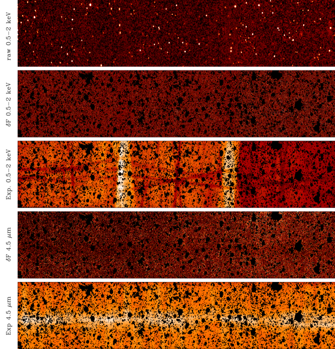
Figure 1: From top to bottom : X-ray 0.5-2 keV count-rate map, smoothed with a Gaussian kernel of 3.6^′′ (3 pixels). X-ray 0.5-2 keV fluctuation maps in counts rate units. The X-ray exposure map. IRAC 4.5 $\mu$m fluctuation map. The IRAC 4.5 $\mu$m exposure map. In all maps the black areas represent the mask. The EGS field is located at Celestial / Ecliptic / Galactic coordinates of (214.91$\arcdeg$, 52.43$\arcdeg$), (180.56$\arcdeg$, 60.00$\arcdeg$), (95.95$\arcdeg$, 59.81$\arcdeg$) and these sub-images cover $45{{}^{\prime}}\times 8{{}^{\prime}}$.

The Spitzer Space Telescope is a 0.85 m diameter telescope launched into an earth-trailing solar orbit in 2003 (Werner et al., 2004). For nearly 6 years, as it was cooled by liquid He, its three scientific instruments provided imaging and spectroscopy at wavelengths from 3.6 to 160 $\mu$m. In the time since the He supply was exhausted, Spitzer has continued to provide 3.6 and 4.5 $\mu$m imaging with its Infrared Array Camera (IRAC). IRAC has a $5^{\prime}\times 5^{\prime}$ field of view, and a pixel scale of $1.2^{\prime\prime}$, which slightly undersampled the instrument beam size of $\sim 2^{\prime\prime}$ FWHM (Fazio et al., 2004).

The procedure for map assembly is described in our previous papers (Kashlinsky et al., 2005, 2007a) with an extensive summary, including all the tests, given in Arendt et al. (2010). Our IRAC mosaics are prepared from the basic calibrated data (BCD) product using the least-squares self-calibration procedure described by Fixsen, Moseley & Arendt (2000). The preparation and properties of the IR data obtained in the course of the SEDS program and used here are discussed in Kashlinsky et al. (2012). The SEDS program was designed to provide deep imaging at 3.6 and 4.5 $\mu$m over a total area of about 1 square degree, distributed over 5 well-studied regions (Fazio et al., 2011). The area covered is about ten times greater than previous Spitzer coverage at comparable depth. While the main use of the SEDS data sets will be the investigation of the individually detectable and countable galaxies, the remaining backgrounds in these data are well-suited for CIB studies, by virtue of their angular scale, sensitivity and observing strategies. Because of the sufficiently deep coverage with both Chandra and Spitzer observations, we have selected the Extended Groth Strip (EGS; Spitzer Program ID = 61042) field for this analysis. The field is located at moderate to high Galactic latitudes to minimize the number of foreground stars and the brightness of the emission from interstellar medium (cirrus). It also lies at relatively high ecliptic latitudes, which helps minimize the brightness and temporal change in the zodiacal light from interplanetary dust. The observations were carried out at three different epochs, spaced 6 months apart. At each wavelength, the frames are also processed in several different groups to provide multiple images that can be used to assess random and systematic errors. The noise is obtained by separating the full sequence of frames into the alternating even and odd frame numbers. Comparison of these “A” and “B” subsets, through construction of ${\frac{1}{2}}($A-B$)$ difference maps, provides a good diagnostic of the random instrument noise because the A and B subsets only differ by a mean interval of $\sim 100$s.

We also examined shallower ($\sim 3$ hr integration) 5.8 and 8 ${\mu{\rm m}}$ observations of the EGS field that were obtained during Spitzer’s cryogenic mission (program ID = 8). However, even with application of the self-calibration, we find that the resulting images have background problems. Some of the problems are likely to be intrinsic and related to cirrus, i.e. thermal emission from interstellar dust. These observations cover a longer strip of the EGS than the SEDS observations. At the extreme end of the 8 ${\mu{\rm m}}$ image ($\sim 0.5\arcdeg$ from the SEDS region) there is clearly diffuse emission from cirrus, which is also evident in the IRAS 100 ${\mu{\rm m}}$ images and the LAB HI images (Neugebauer et al. 1984; Kalberla et al. 2005). The 5.8 ${\mu{\rm m}}$ data show additional background problems that are not correlated with the 8 ${\mu{\rm m}}$ data. These problems appear to be related to greater instability of the detector offset at 5.8 ${\mu{\rm m}}$, which can be confused with temporal changes in the zodiacal light. Self-calibrating the 5.8 ${\mu{\rm m}}$ data without the subtraction of the estimated zodiacal light normally applied by the BCD pipeline provides a better, but still not satisfactory, result. The background issues at both 5.8 and 8 ${\mu{\rm m}}$ may be compounded by the observing strategy. The SEDS strategy stepped across the full length of the field relatively quickly, and then accumulated depth by repeated observations, while the cryogenic observations accumulated the full depth of coverage at each pointing before moving on to another location along the EGS field. Because of these background issues and the higher noise levels in these data, cross correlations of 5.8 and 8 ${\mu{\rm m}}$ emission with X-ray emission did not yield any significant results to present in this paper.

The region selected for the joint CXB-CIB analysis is about $\sim 8^{\prime}\times 45^{\prime}$ in size. The common mask from the IRAC 3.6$\mu$m and 4.5$\mu$m bands and the X-ray bands was used, with about $\simeq 32\%$ of the pixels lost to the analysis. An example of the CIB fluctuation maps is shown in Fig. 1.

3 Fluctuation analysis

3.1 Definitions

The maps under study are clipped and masked for the resolved sources, yielding the fluctuation field, $\delta F(\vec{x})$. The Fourier transform, $\Delta(\vec{q})=\int\delta F(\vec{x})\exp(-i\vec{x}\cdot\vec{q})d^{2}x$ is calculated using the FFT. The power spectrum in a single band $n$ is $P_{n}(q)=\langle|\Delta(\vec{q})|^{2}\rangle$, with the average taken over all the independent Fourier elements which lie inside the radial interval $[q,q+dq]$. Since the flux is a real quantity, only one half of the Fourier plane is independent, so that at each $q$ there are $N_{q}/2$ independent measurements of $\Delta(\vec{q})$ out of a full ring with $N_{q}$ data. A typical rms flux fluctuation is $\sqrt{q^{2}P_{n}(q)/2\pi}$ on the angular scale of wavelength $2\pi/q$. The correlation function, $C(\theta)=\langle\delta F(\vec{x})\cdot\delta F(\vec{x}+\vec{\theta})\rangle$, is uniquely related to $P_{n}(q)$ via Fourier transformation. If the fraction of masked pixels in the maps is too high, the large-scale map properties cannot be computed using the Fourier transform and instead the maps must be analyzed by direct calculation of $C(\theta)$, which is immune to mask effects. In this study, the clipped pixels occupy $\simeq 32\%$ of the maps which allows for a robust FFT analysis; this issue has been addressed in great detail in the context of the Spitzer-based CIB studies in Kashlinsky et al. (2005); Arendt et al. (2010); Kashlinsky et al. (2012).

We characterize the similarity of the fluctuations measured in different bands via the cross-power spectrum, which is the Fourier transform of the cross-correlation function $C_{mn}(\theta)=\langle\delta F_{m}(\vec{x})\cdot\delta F_{n}(\vec{x}+\vec{\theta})\rangle$. The cross-power spectrum is then given by $P_{mn}(q)=\langle\Delta_{m}(q)\Delta^{*}_{n}(q)\rangle={\cal R}_{m}(q){\cal R}_{n}(q)+{\cal I}_{m}(q){\cal I}_{n}(q)$ with ${\cal R,I}$ standing for the real, imaginary parts. Note the cross-power of real quantities, such as the flux fluctuation, is always real, but unlike the single (auto-) power spectrum the cross-power spectrum can be both positive and negative.

The errors on the power have been computed by using the classical Poissonian estimators so that for the auto-power $\sigma_{P_{n}}(q)={P_{n}}(q)/\sqrt{0.5\,N_{q}}$ and for the cross-power $\sigma_{P_{mn}}(q)=\sqrt{{P_{m}}(q){P_{n}}(q)/N_{q}}$. These errors have been verified to be accurate to better than a few percent from comparison to the intrinsic standard deviation of the Fourier amplitudes at the various $q$.

3.2 CXB power spectra

The analysis of the fluctuations of the CXB has been performed in the Chandra [0.5-2] keV, [2-4.5] keV and [4.5-7] keV bands. We evaluated the power spectra and their relative errors from the individual Chandra masked maps as well as from the ${{\frac{1}{2}}(A-B)}$ image. The final power spectrum of CXB fluctuations, $P_{X}$, is therefore evaluated as $P_{{\frac{1}{2}}(A+B)}-P_{{\frac{1}{2}}(A-B)}$ with correspondingly propagated errors. The X-ray count maps, however, have an occupation number of $<$1 cts/pix, so the Gaussian behavior of their variance is not guaranteed especially at small scales. Correspondingly, we evaluated the mean number of photons per $N_{q}/2$ elements in the Fourier domain.

The left panel of Figure 2 shows the number of independent Fourier elements, $N_{q}/2$, as a function of $2\pi/q$. The right panel shows the mean number of X-ray photons per element [i.e. $N_{cts}/(N_{q}/2)$] as function of angular scale, where $N_{cts}\approx 135000$ (Tab. 1). A limit of 20 cts/element is taken as a practical division between Gaussian and Poissonian regimes. The figure shows that below 10^′′, X-ray counts are in the Poissonian regime, and therefore we limit our analysis of auto- and cross-power spectra to scales $>10{{}^{\prime\prime}}$ to avoid biases introduced by low-count statistics.

Figure 2: Left: Number of independent Fourier elements per bin that went into determining the power spectrum for each field. Right: The average number of photon counts per Fourier element adopted for determining the power spectrum as function of angular scale.

In order to take into account the effects of sensitivity variation across the field of view, in every pixel the fluctuation field $\delta F_{x}(i)$ has been weighted by a factor $E(i)/\langle E\rangle$ where $E(i)$ is the effective exposure at the pixel $i$ and $\langle E\rangle$ is the mean exposure in the field. The clipped and cleaned maps were Fourier transformed and power spectra evaluated.

The binning of the power spectrum in angular scale is the same for all the energies sampled here. The relative sampling error (cosmic variance) on the determined power is $[{\frac{1}{2}}N_{q}]^{-{\frac{1}{2}}}$, and so the power spectrum is not determined highly accurately at the largest angular scales ($\gtrsim 250^{\prime\prime}$) of the EGS field where ${\frac{1}{2}}N_{q}{{}_{<}\atop{}^{\sim}}10$. The X-ray power spectra measured in the three X-ray energy bands are shown in Fig. 3.

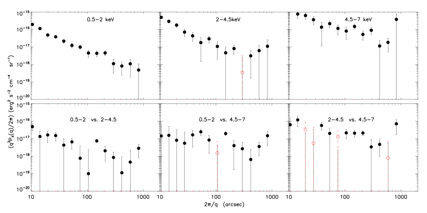
Figure 3: Source-subtracted CXB fluctuation power spectra ($top~{}row$) in the [0.5-2] keV, [2-4.5] keV and [4.5-7] keV energy bands and their relative cross-power spectra ($bottom~{}row$). Open red circles and error bars represent the negative power points shown in absolute value for a better highlighting of the signal.

The [2-4.5] keV and [4.5-7] keV power spectra are noisier than that measured in the [0.5-2] keV band since in those bands the particle background is dominant with respect to CXB. In order to probe whether the source-subtracted maps at the different energy bands contain the same populations, we computed the cross-power spectrum between each pair of maps. This analysis shows that the cross-power spectra between the hard bands and the [0.5-2] keV band generally have lower amplitudes than the corresponding auto-power spectra, especially on smaller scales. This suggests that the population of sources producing the [0.5-2] keV CXB fluctuations can be substantially different from that producing the hard X-ray CXB. Such a conclusion can be confirmed by computing the level of coherence of the signal of every band pairs. As in Kashlinsky et al. (2012) we can express the common contribution of the sources to both IR and X-ray signals in terms of coherence, ${\cal C}(q)=\frac{|P_{\rm m,n}(q)|^{2}}{P_{\rm m}(q)P_{\rm n}(q)}$. The coherence can also be interpreted as the fraction of the emission due to the common populations so that ${\cal C}\sim\zeta_{m}^{2}\zeta_{n}^{2}$, where $\zeta_{m}$ and $\zeta_{m}$ are the fractions of the emissions produced by the common population in the probed $m$ and $n$ X-ray bands. As a result, we find that for the band pairs [0.5-2] keV/[2-4.5] keV and [0.5-2] keV/[4.5-7] keV, ${\cal C}\sim$0.1 and ${\cal C}\sim$0.05, respectively. Thus only 30% of the [0.5-2] keV emitters contribute also to the [2-4.5] keV power, while $<20\%$ of the [0.5-2] keV emitters contribute also to the [4.5-7] keV power. The mean level of coherence between [2-4.5] keV and [4.5-7] keV is ${\cal C}\sim$0.3-0.4, but with large uncertainties.

It is important to emphasize, in the context of the discussion below (Sect. 4.), that the interpretation of the CXB power and cross-power spectrum carries an intrinsic source of uncertainty due to the contribution of the Galaxy. Thus, the results shown in Fig. 3 for individual bands present an upper limit on the unresolved extragalactic CXB fluctuations because they contain the contribution from the Galaxy which is more prominent at the softest energies. Although our inspection of ROSAT Galaxy diffuse emission maps in this field does not show any well defined structure, the actual shape of the Galaxy’s diffuse emission power spectrum is unknown on these scales. Śliwa et al. (2001) measured the power spectrum of the ROSAT soft X-ray background fluctuations and showed that its shape and amplitude is a strong function of the Galactic coordinates. However, their measurements were obtained on scales larger than $\sim$10^′ limiting any direct comparison to the CXB fluctuations in our field. Nevertheless, their Fig. 9 shows that the Galaxy component, at high Galactic latitudes, is approximately white noise at sub-degree scales. A more accurate measurement will be possible only with the forthcoming launch of eROSITA (Predehl et al., 2010) in late 2014. Thus, while irrelevant for the CXB-CIB cross-power spectrum (see below), correcting for the Galaxy would reduce our estimate of the extragalactic CXB auto-power spectrum, particularly on the smallest scales. Since the Galaxy mostly emits below 1 keV, this could be the reason for a low-level of cross-correlation between [0.5-2] keV and [2-4.5] keV-[4.5-7] keV maps.

3.3 CIB power spectra

In Fig. 4 we show the auto-power spectra of the IRAC 3.6$\mu$m and 4.5$\mu$m maps and their cross-power power spectrum. The CIB fluctuation spectra evaluated in this work are in excellent agreement with those derived by Kashlinsky et al. (2012) in the original EGS field even with the additional masking of X-ray detected sources. Power spectra with or without the additional X-ray masking agree to better than $5\%$ on all scales, as shown by solid symbols and green lines. This is consistent with the populations responsible for the CIB fluctuation signal being unrelated to the remaining known galaxy or galaxy cluster populations in the field.

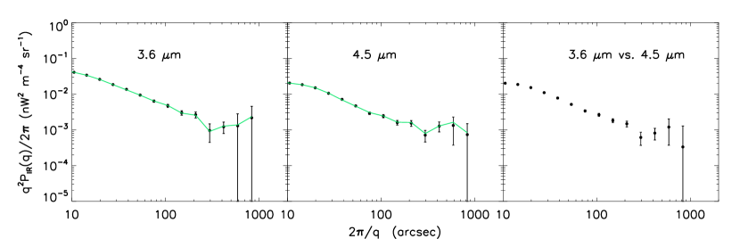
Figure 4: Left and central panels: The 3.6 $\mu$m and 4.5 $\mu$m CIB fluctuations power spectra, respectively in the EGS field. Right: 3.6 $\mu$m vs 4.5 $\mu$m fluctuations cross-power spectrum in the EGS field. Green lines show CIB fluctuations evaluated after applying only the IR mask (instead of the IR+X-ray mask) to the data as in Kashlinsky et al. (2012).

3.4 CIB-CXB cross-power spectra

In order to establish if the fluctuations in the source-subtracted CXB and CIB maps have been totally or partly produced by a population of sources sharing the same environment (or even being the same sources), we performed the cross-power analysis and evaluated $P_{\rm IR,X}(q)$. Since the X-ray and IR noise are uncorrelated, the cross-power of the instrument noise contributions should alternate around zero. The cross power-spectrum between IRAC 3.6$\mu$m and 4.5$\mu$m  source-subtracted CIB fluctuations and Chandra [0.5-2] keV fluctuations are shown in Fig. 5, where we find a statistically significant cross-power. The same is plotted for IRAC 3.6$\mu$m and 4.5$\mu$m versus Chandra [2-4.5] keV and Chandra [4.5-7] keV, in Fig. 6, where we do not find statistically significant detection.

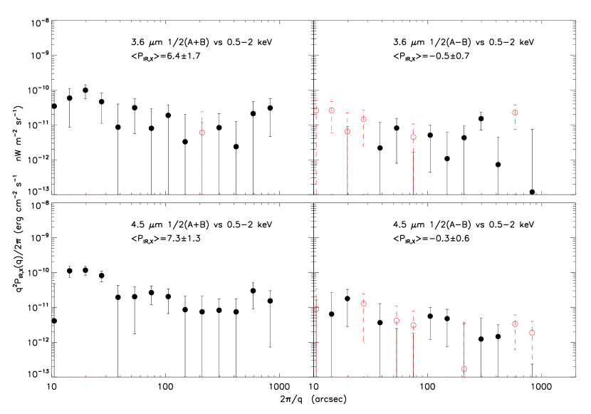
Figure 5: (Top left) The fluctuations cross-power spectrum between IRAC 3.6 $\mu$m $\frac{1}{2}$($A+B$) and Chandra [0.5-2] keV. (Top Right) The fluctuations cross-power spectrum between IRAC 3.6 $\mu$m $\frac{1}{2}$($A-B$) and Chandra [0.5-2] keV. The bottom row shows the same, but for IRAC 4.5 $\mu$m and Chandra [0.5-2] keV. The labels in the plots list the average cross-power measured on the angular range 10^′′-1000^′′ in units of 10^-20 $\rm erg/cm^{2}/s\$nW m^-2 sr^-2. Open red circles and dashed red error bars represent the absolute values of negative power points.

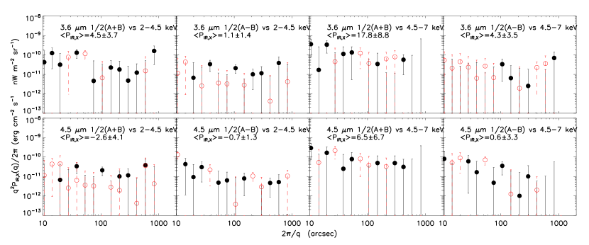
Figure 6: Same as Fig. 5 but for the [2-4.5] keV band (left panels) and [4.5-7] keV band (right panels). Note that in these hard X-ray bands the measured cross power is consistent with zero in all cases.

We evaluated the overall significance of the cross-power by averaging the results over the whole angular range ($10^{\prime\prime}<2\pi/q<1000^{\prime\prime}$), computing the mean and its standard deviation. We also evaluated the significance from the actual dispersion of the un-binned data and found identical results. In Fig. 7 we display the full 2-dimensional cross power spectrum, $P_{\rm IR,X}(\vec{q})$, for 4.5 $\mu$m and [0.5-2] keV. The mean power-spectra for every band pair investigated here are reported in Tab. 2. We find mean correlations at $\sim$3.8$\sigma$ and 5.6$\sigma$ significance between the [0.5-2] keV band and IRAC 3.6 and 4.5 ${\mu{\rm m}}$ bands respectively. Stripe-type artifacts and gradients in the images are mapped onto axes in the Fourier representation. So although the Fourier maps look reasonably clean, we also evaluated the CIB vs. CXB cross-power after masking the axes in the Fourier domain. The results are consistent within 1$\sigma$ with those reported in Tab. 2, although less significant because of the reduced number of data points introduced by such a masking.

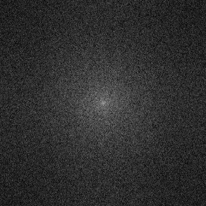
Figure 7: The unbinned 2-dimensional $|P_{\rm IR,X}(q)|$ for 4.5 $\mu$m vs [0.5-2] keV is shown in the left panel with a logarithmic scale. The frequency space spans $-2\pi/2.4^{\prime\prime}<q<2\pi/2.4^{\prime\prime}$ on each axis. The right panel zooms in on the low-frequency (large-scale) part of $P_{\rm IR,X}(q)$ for $-2\pi/38.4^{\prime\prime}<q<2\pi/38.4^{\prime\prime}$, shown on a linear scale. Here the frequency space pixels are clearly not square because of the rectangular shape of the original image. The figures show that at both small and large spatial scales, there are not evident artifacts (e.g. asymmetries or large outliers) in the 2-D cross-power that would affect the binned 1-D result (Fig. 5, lower left).

The [2-4.5] keV and [4.5-7] keV bands do not show significant cross-correlation with IRAC band as shown in Tab. 2. We tested if the observed cross-correlation could have been produced by spurious instrumental features by cross-correlating the X-ray ${\frac{1}{2}}($A+B$)$ maps with ${\frac{1}{2}}($A-B$)$ IR maps and computed their average cross-power for every X-ray and IR band pair. The results of this analysis are plotted in Figs. 5 and 6 and listed in Tab. 2. We note that these cross-power spectra are always consistent with zero and, as far as 3.6 $\mu$m and 4.5 $\mu$m versus [0.5-2] keV bands are concerned, the detected signal in the data is much larger than the cross-correlation between X-ray and IR noise maps. This cross correlation provides an estimate of the noise contribution for our analysis and a probe for systematic spurious power in the data.

Table 2: Mean P_IR,X in units of 10^-20$\rm erg/cm^{2}/s\$nW m^-2 sr^-1 computed over the [10^′′-1000^′′] angular range.

Bands	0.5–2 keV			2–4.5 keV			4.5–7 keV
$E_{\rm eff}$	1.2 keV			3.2 keV			2.3 keV
	$\langle P_{IR,X}\rangle$	$\langle P_{{\frac{1}{2}}A-B,X}\rangle$		$\langle P_{IR,X}\rangle$	$\langle P_{{\frac{1}{2}}A-B,X}\rangle$		$\langle P_{IR,X}\rangle$	$\langle P_{{\frac{1}{2}}A-B,X}\rangle$
3.6${\mu{\rm m}}$	6.4$\pm{{\bf 1.7}}$	-0.5$\pm{0.7}$		4.5$\pm{3.7}$	1.1$\pm{1.4}$		17.8$\pm{8.8}$	4.3$\pm{3.5}$
4.5${\mu{\rm m}}$	7.3$\pm{{\bf 1.3}}$	-0.3$\pm{0.6}$		-2.6$\pm{4.1}$	-0.7$\pm{1.4}$		6.5$\pm{6.7}$	0.6$\pm{3.3}$

Note. — Bold text indicates the statistically significant results.

We also have cross correlated the CIB fluctuations with our particle background model. For the 3.6 $\mu$m and 4.5 $\mu$m vs. [0.5-2] keV band pairs, the cross power spectra have amplitudes of ($-2.7\pm{2.2})\times$10^-20$\rm erg/cm^{2}/s\$nW m^-2 sr^-1 and (0.7$\pm{1.6})\times$10^-20$\rm erg/cm^{2}/s\$nW m^-2 sr^-1 respectively and thus cannot account for the observed signal. To further check the robustness of our results we also calculated cross-power spectra of our X-ray images with 1,000 random CIB fluctuation maps constructed by resampling the original masked maps. In Fig. 8 we show that, at every scale, no statistically significant cross-power signal can be recorded.

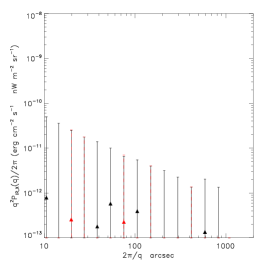
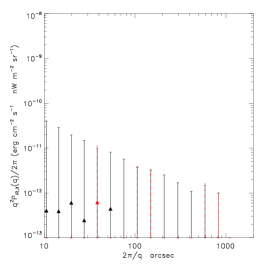
Figure 8: Left panel: The mean [0.5-2] keV vs 3.6 $\mu$m cross power obtained with 1000 Monte Carlo simulations and its standard deviation; the absolute values of negative cross-powers are plotted in red. The same is plotted in the central panel but referred to [0.5-2] keV vs 4.5 $\mu$m cross power. In the right panel we show the relation between errors measured with the actual dispersion of the Monte Carlo realizations ($x$-axis) and that measured with our estimator ($y$-axis).

Moreover such a test confirms that the amplitude of the estimated errors are consistent with the errors obtained by measuring the dispersion of the power in Fourier space. To illustrate this we show, in the right panel of Fig. 8, that the errors estimated from the dispersion of the measurement in the Monte Carlo simulation are equivalent to those derived from our estimates. In a final test we divided the field in two equal parts (left and right sides in Fig. 1) and recomputed the cross-power between [0.5-2] keV and 3.6 $\mu$m and 4.5 $\mu$m. On the left side we obtain P_IR,X=(5.7$\pm{2.3})\times$10^-20$\rm erg/cm^{2}/s\$nW m^-2 sr^-1 and (8.2$\pm{1.8})\times$10^-20$\rm erg/cm^{2}/s\$nW m^-2 sr^-1 for the [0.5-2] keV vs. 3.6 $\mu$m and [0.5-2] keV vs. 4.5 $\mu$m, respectively. On the right side of the field we obtain P_IR,X=(7.9$\pm{2.7})\times$10^-20$\rm erg/cm^{2}/s\$nW m^-2 sr^-1 and (5.0$\pm{1.8})\times$10^-20$\rm erg/cm^{2}/s\$nW m^-2 sr^-1 for [0.5-2] keV vs. 3.6 $\mu$m and [0.5-2] keV vs. 4.5 $\mu$m, respectively. While the lower number of independent Fourier elements makes the measurements in the two smaller sub-fields less significant, the amplitudes of the cross-power spectra are consistent when measured in different parts of the field.

4 Discussion

The source-subtracted CIB fluctuations are made up of two components: 1) small scales (${{}_{<}\atop{}^{\sim}}20^{\prime\prime}$ are dominated by the shot-noise from all sources (known and new) below the removal threshold, while 2) the larger angular scales reflect CIB fluctuations produced by the clustering of the new populations (Kashlinsky et al., 2007b). Thus the coherence between the two components of the fluctuations may be different depending on the different common levels of the populations producing the two terms. However, it is the larger scales, where the cross-power is due to clustering of the new populations common to both IR and X-ray emissions which are of greatest interest to interpret here.

At large angular scales (${{}_{>}\atop{}^{\sim}}20^{\prime\prime}$), where the clustering term dominates the CIB fluctuations spectrum, the coherence between 4.5$\mu$m and [0.5-2] keV is ${\cal C}\sim 0.02-0.05$. The coherence at 3.6 $\mu$m versus [0.5-2] keV is consistent with these values, although the cross-power is less statistically significant.

Because the measured cross-power between the 4.5$\mu$m and X-ray data is highly positive, we plot in Fig. 9 the CIB fluctuations produced by sources common to both the source-subtracted CIB at 4.5 $\mu$m and the [0.5-2]keV CXB, i.e. $P_{\rm CIB,common}=P_{\rm IR,X}^{2}/P_{\rm X}\equiv{\cal C}\times P_{\rm IR}$. This assumes that all of the CXB power spectrum is produced by these sources and implies a lower limit on the CIB fluctuations contributed by the common sources. The figure shows that ${{}_{>}\atop{}^{\sim}}15-25\%$ of the CIB power spectrum can be accounted for by these sources. The rightmost panel of Fig. 9 gives a similar plot for the minimal contribution, $P_{\rm CXB,common}=P_{\rm IR,X}^{2}/P_{\rm IR}\equiv{\cal C}\times P_{\rm X}$, to the CXB from the common populations. If we consider that the CXB power spectrum may be contaminated by the foreground contribution of the Galaxy that at the moment, is not possible to model, the fraction of CIB power produced by X-ray sources quoted above must be considered as a lower limit. We must emphasize that the “common population” does not necessarily imply that the corresponding parts of the CIB and CXB are produced by the same physical sources emitting at both IR and X-rays. With the map resolution of a few arcsec we cannot resolve the individual point sources, especially if they are at high $z$. This is further amplified since the Gaussian regime of the X-ray maps is reached at angular scale of $\simeq 10^{\prime\prime}$ which subtend linear scale of $\sim 0.1h^{-1}$Mpc at $z\sim$1 and this defines the scale of the individual “objects” in our analysis and the discussion below. Thus we cannot resolve whether the IR and X-ray emitters are one and the same or whether they are different sources that share the same environment at the relevant angular scales. Moreover, from the amplitude of the cross-correlation signal itself it is not possible to directly determine if the signal is produced by a single population of sources, or if it is produced by different populations sharing the same environment.

4.1 Galactic, solar system, and instrumental foregrounds

We begin by considering possible non-cosmological contributions to the detected cross-correlation. In the IR bands, the most significant foreground source of fluctuations would come from the Galactic cirrus emissions. Yet, it was demonstrated by Kashlinsky et al. (2012) that the bulk of the measured 3.6$\mu$m and 4.5$\mu$m power cannot be produced by cirrus. Cirrus emission is produced by dust in cold neutral and molecular clouds which cannot emit X-rays, but can be effective absorbers of the soft X-ray background leading to a negative contribution to the positive cross-power that is measured (Wang & Yu, 1995; Snowden et al., 2000). The Galactic X-ray emission from the hot phase of the ISM could play a role in the cross power, but there are several factors that limit its contribution to the cross power: 1) It is well known that the hot ISM mostly emits soft X-rays with energy $<$1 keV (Snowden et al., 1995), and thus would be relatively weak even in the [0.5-2] keV band; 2) the Galactic X-ray background shows clustering on scales on the order of one degree, which is larger than the scales of interest here; and 3) the dust producing the IR emission is in the cold phases of the ISM, and thus should be anti-correlated with the hot ISM, leading to negative cross-power.

Very faint Galactic stars could, in principle, contribute to the cross-power. However at high Galactic latitudes Lehmer et al. (2012) showed that stars are a negligible component of the unresolved CXB. Moreover, the high level of isotropy of the CIB fluctuations works against the hypothesis of any Galactic sources as the possible sources of CIB fluctuations.

Other possible sources of contamination discussed by Kashlinsky et al. (2012) are zodiacal light and instrumental stray light whose contributions to CIB fluctuations which were demonstrated to be negligible. At a low level, the IR zodiacal light may correlate with Solar System X-rays generated by solar wind charge exchange (SWCX). However, SWCX primarily produces very low surface brightness O VII emission around 0.54 keV where the Chandra effective area is very low and should not produce such a high signal. Moreover SWCX emission is time dependent and therefore since Spitzer and Chandra observed the field at different epochs, the signals are unlikely to show a correlation due to solar system effects.

To summarize, our analysis points to an extragalactic origin of the positive cross-power spectra between the soft X-rays and the 3.6 and 4.5 ${\mu{\rm m}}$ background fluctuations.

4.2 Extragalactic populations

Several classes of extragalactic populations could contribute to the observed CXB-CIB cross-correlation. Below we briefly discuss the most obvious candidates for the emissions. More detailed interpretation will be worked out elsewhere, although it already appears that some of the candidates can be safely ruled out. For proper interpretation of the measured CIB-CXB correlation it is important to reiterate the limits imposed from the IR analysis itself. The sources in the IRAC maps used here are removed down to the shot-noise $P_{\rm SN}\simeq 30$ nJy$\cdot$$\rm~{}nW/m^{2}/sr$ (Kashlinsky et al., 2012), which is equivalent to sources removed to magnitudes of $m_{\rm AB}\simeq 25-25.5$ (Kashlinsky et al., 2005; Helgason et al., 2012). Therefore, for this discussion we adopt as the flux limit of $S_{\rm lim}\sim 300$nJy at the IRAC bands. Thus in order to account for the measured CIB fluctuation of $\delta F\sim 0.05-0.1$$\rm~{}nW/m^{2}/sr$ these sources must have projected angular number density $n{{}_{>}\atop{}^{\sim}}\delta F/S_{\rm lim}\times(\delta F/F)^{-1}$ where $F\sim nS$ is the CIB level produced by them. The remaining CIB sources below the threshold would have to have $n{{}_{>}\atop{}^{\sim}}(0.3-0.4)[(S_{\rm lim}/300{\rm nJy})(\delta F/F)]^{-1}$arcsec^-2 in order to explain the observed CIB at 3.6-4.5 $\mu$m. Only the sources that can produce highly non-linear CIB fluctuations, $\delta F/F\gg 1$ all the way to sub-degree scales, can have projected number density significantly lower than this. The CIB from such sources would, however, then exhibit a clear void-cluster CIB pattern contrary to what we see in the CIB maps. Consequently our measurements indicate that in order to explain the detected cross-correlation the sources producing them would have to account for ${{}_{>}\atop{}^{\sim}}\sqrt{{\cal C}}$ or ${{}_{>}\atop{}^{\sim}}15-25\%$ of the CIB signal and be abundant enough to reproduce the required number density while accounting for the remaining CXB fluctuation.

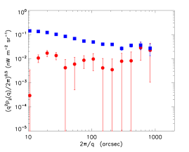
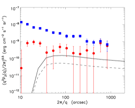
Figure 9: ($left$): The IRAC 4.5 $\mu$m fluctuation power spectrum (blue squares) compared with the 4.5 $\mu$m power from accreting sources (red circles). ($right$): The Chandra [0.5-2] keV fluctuation power spectrum (blue squares) compared with the power-spectrum of X-ray sources correlating with IR 4.5 $\mu$m CIB. (red circles). The dotted line is the expected upper-limit for power spectrum for remaining X-ray normal galaxies with $m_{AB}>25$ at 4.5 $\mu$m and $X/O<-1$. The dashed line is the expected upper-limit for power spectrum for remaining AGN with m${}_{AB}>$25 at 4.5 $\mu$m and $X/O<0$. The continuous line is the sum of the AGN and galaxies fainter than $m_{AB}\sim 25-25.5$.

4.2.1 Diffuse gas in clusters and WHIM

As mentioned in the introduction, the sources of the unresolved soft X-ray CXB power are mostly galaxy groups and the putative WHIM (Warm Hot Intergalactic Medium; Cen & Ostriker, 1999). However the mass limit of our source detection allows us to exclude from our analysis extended sources with mass $M>10^{13}{{\rm M_{\odot}}}$. Galaxy cluster scaling relations (see e.g., Pratt et al., 2009) ensure in this case that these sources have a low $kT$ (i.e. ${{}_{<}\atop{}^{\sim}}1$ keV). Any sources correlated with clusters of galaxies at even marginally high $z$, would require the gas to be at temperatures shifted upward by a factor of $(1+z)$, making the origin in this component even less likely, doubly so since the clusters/groups are expected to have colder gas at the early times. We therefore conclude that such a population cannot be responsible for these measurements. This is further confirmed by the fact illustrated in Fig. 4 which shows that the additional X-ray masking, which includes the resolved X-ray sources, does not have any noticeable effect on the measured CIB fluctuations. Similarly, the WHIM, although it has never been significantly detected in emission, is expected to show a typical emission line dominated spectrum. Most of the emission is produced by H-, He-like O and Ne like ions, which emit at energies below $<$ 700 eV. We also note that the diffuse sources producing the CXB peak at $z\sim 0.1$. If the observed cross-correlation arose at that redshift, then the IR sources would be a population of still undetected numerous low luminosity (i.e. with L$\sim$10⁷ $L_{\odot}$, Kashlinsky et al., 2007b) galaxies, which further weakens this low-$z$ hypothesis.

4.2.2 X-ray emission in remaining “normal” galaxies

X-ray binaries and supernova remnants are the main sources of X-rays from normal galaxies. It has been shown that this population emits X-ray with a typical spectrum $n(E)\propto E^{-2}$ (Ranalli et al., 2005). Therefore their emission could contribute to the whole energy range sampled here. Although it is not straightforward to determine the effective X-ray flux of galaxies with IR counterparts at $m_{\rm AB}{{}_{>}\atop{}^{\sim}}25-25.5$, a useful tool to determine the effective X-ray brightness of galaxies below this magnitude limit is the X-ray to optical (2500Å) ratio ($X/O$). In fact, it has been shown that for X-ray sources, the X-ray to optical/IR flux ratio assumes well defined values according to the nature of the sources.

The $X/O$ is defined as $X/O=\log(f_{X}/f_{\rm opt})=\log(f_{X})+C+m_{Vega}/2.5$. For the 4.5$\mu$m  vs [0.5-2] keV band the constant $C$ has a value of $\sim$7.53 (Civano et al., 2012). For observations with a depth comparable with ours, the value of $X/O$ for normal galaxies is $X/O\ll-1$ (Xue et al., 2011). Thus X-ray galaxies with IR counterpart with $m_{\rm AB}{{}_{>}\atop{}^{\sim}}25-25.5$ should have the [0.5-2] keV flux $f<3-4\times 10^{-18}{\rm erg/cm^{2}/s\ }$, which is about one order of magnitude below the flux limit of the 4Ms CDFS (Xue et al., 2011) and $\sim 20$ times fainter than our limit for the EGS field.

In order to determine if these faint X-ray sources could produce the observed fluctuations we adopted the recipe of Cappelluti et al. (2012) and computed the expected CXB fluctuations angular auto-power spectra produced by the clustering component of these sources, i.e. the power in the X-ray bands from normal galaxies below $z\sim 7.5$ and $f([0.5-2]{\rm keV})<3-4\times 10^{-18}{\rm erg/cm^{2}/s\ }$. This contribution, which is of the order of 2-3% of the total CXB power, is shown in Fig. 9, right and is systematically small compared to the measured power on scales $20^{\prime\prime}-200^{\prime\prime}$.

Additional evidence against a significant contribution of normal galaxies is: 1) the shot-noise component in the CIB fluctuations on small scales, which is dominated by the undetected normal galaxies, appears uncorrelated with that in the CXB as is shown by the drop in the correlated power at the smallest scales (see Fig. 9), and 2) on large scales, which are dominated by the clustering component, the minimal CIB fluctuation shown in Fig. 9 appears larger than the normal galaxy component reconstructed by Helgason et al. (2012) as displayed in the lower right of Fig. 9 of Kashlinsky et al. (2012).

Thus normal galaxies could be responsible only for a small part of the observed signal.

4.2.3 Remaining known AGNs

AGNs are characterized by strong IR emissions due to reprocessing gas in the nuclear regions (torus) (Elvis et al,, 1994), and/or the contribution of star forming processes in the host galaxy. The contributions to the CIB from these sources at intermediate $z\sim 2-4$ would arise from the IR bump produced by hot dust with maximum temperature of $\sim 10^{3}$ K.

One should therefore consider whether known AGNs can be responsible for the observed cross-correlation between the source-subtracted CIB and CXB. A critical point in estimating their contribution to the measured cross-power is that the signal is produced by sources below the IR flux of $S_{\rm lim}\simeq 300$ nJy at 3.6 and 4.5 $\mu$m which is fixed by the measured shot-noise level remaining in the CIB maps (Kashlinsky et al., 2005; Helgason et al., 2012; Kashlinsky et al., 2012). Treister et al (2004, 2006) conducted a detailed Spitzer/IRAC-based census and modeling of the Type I and II AGNs in the GOODS region and their results show that one expects the total number density of Type I and II AGNs to be $n_{\rm AGN}\simeq 6000$deg^-2 at the IR fluxes below $S_{\rm lim}$. The CIB flux at 3.6 and 4.5 $\mu$m from the undetected AGNs is then $I_{\rm AGN}\simeq n_{\rm AGN}S_{\rm lim}=6\times 10^{-6}$MJy/sr or $F_{\rm AGN}=0.004$ nW/m²/sr at 4.5 ${\mu{\rm m}}$. Thus if the AGNs were to produce the measured CIB signal of $\delta F\simeq 0.05$ nW/m²/sr at 4.5$\mu$m at sub-degree scales (Kashlinsky et al., 2012), with their X-ray emissions accounting for the observed cross-power, the resultant CIB would have to have highly non-linear fluctuations on scales between 1^′ and 1^∘ with $\delta F/F{{}_{>}\atop{}^{\sim}}10$. A possibility would be that the signal could be produced by a population of faint CIB galaxies correlating with highly biased high-$z$ AGN.

A new study Xue et al. (2012) reported a significant contribution to the unresolved CXB ($\sim$25%) at [6-8]keV from highly absorbed AGN with very faint optical counterpart ($25<m<28$ at 0.85$\mu$m). The quoted result is at 3.9$\sigma$ significance at [6-8] keV, while these populations are not detected below 4 keV. Thus they cannot be responsible for the observed effect since the correlated maps are all at energies effectively much below 6 keV. We further emphasize that only sources with 3.6 and 4.5$\mu$m fluxes below $S\sim 300$ nJy contribute to the measured fluctuations. Obscured AGN are the most abundant sources among faint AGN (Hasinger, 2008). They typically show very hard spectra and weak X-ray emission below $\simeq$ 3-5 keV. Since we did not detect a hard X-ray cross-power spectrum, these sources, if AGNs, would be either Type-I sources or high-$z$ ($z>$2-4) obscured AGN, with their primary power-law component redshifted to the [0.5-2] keV band.

Cappelluti et al (2012) calculated the expected clustering component of the angular auto-power spectrum produced by AGNs with IRAC 4.5$\mu$m counterparts with m${}_{AB}>$25-25.5. The median $X/O$ value for X-ray selected AGN is $\sim$0 (Xue et al., 2011; Civano et al., 2012). Therefore, in order to produce the observed cross-correlation they should have [0.5-2] keV fluxes $<3-4\times 10^{-17}{\rm erg/cm^{2}/s\ }$. By using the recipe of Cappelluti et al. (2012) we evaluated their expected angular auto-power under the assumption that they lie at $z<$7.5. Our prediction is shown in the right panel of Fig. 9. Its amplitude is of the order 7-8% of the total CXB fluctuations observed here. When added to the normal galaxies component this adds up to 10-11% of the total CXB fluctuations which is about 50% of the observed lower limit.

4.2.4 New high-$z$ populations

Although no direct measurement of the redshift of the source-subtracted CIB fluctuations is yet available, there is now a significant body of evidence that the fluctuations may originate at early times of the Universe’s evolution: 1) The measured amplitude of the fluctuations cannot be accounted for by the low-luminosity end of the distribution of “ordinary”/known galaxies (Kashlinsky et al., 2005; Helgason et al., 2012). 2) There are no correlations between the source-subtracted CIB maps at Spitzer wavelengths and HST/ACS data out to 0.9 $\mu$m, which points to $z>7-8$ for the populations producing the large scale excess signal unless the latter comes from new, and so far unobserved, very faint and more local populations at AB mag ${{}_{>}\atop{}^{\sim}}28$ which have escaped the ACS detection (Kashlinsky et al., 2007c). 3) The pattern of the fluctuations is inconsistent with that of the galaxy populations at recent times, and is consistent with the $\Lambda$CDM-distributed sources at high $z$ (Kashlinsky et al., 2007b, c, 2012). 4) The colors of the fluctuations from 2 to 4.5 $\mu$m are consistent with very hot sources at high-$z$ (Matsumoto et al., 2011).

If the X-ray signal comes from sources at high redshifts we clearly do not see direct stellar photospheric emissions, since massive metal-poor stars have $T\simeq(9-10)\times 10^{4}$K (Schaerer et al., 2003), which is not hot enough to contribute to emissions in the observed X-ray bands extending to 7 keV. Instead, if the signal originates from these sources, the contribution to the CXB signal would originate from thermal emission of the gas in accretion disks.

We measure a coherence of ${\cal C}\sim 0.02-0.05$. So if the BHs amongst the sources responsible for the measured source-subtracted CIB fluctuations produce the entire X-ray signal, they should account for $\simeq 15-25\%$ of the signal produced at 4.5 $\mu$m. If they contribute only a fraction of the X-ray fluctuations, their IR contribution would be even higher, but the measured cross-power suggests that $\zeta_{\rm X}{{}_{>}\atop{}^{\sim}}15-25\%$. At the lower limit of $\zeta_{\rm X}$ the accreting sources (BHs?) would need to account for the entire CIB signal at 4.5 $\mu$m (i.e. $\zeta_{\rm IR}=1$).

If the high-$z$ sources are responsible for the detected cross-power, these early X-ray sources were present when the Universe was still partly neutral. Unlike UV photons, X-rays have the capability of multiple ionizations. If the sources responsible for the observed cross-correlation are at high-$z$, we are observing correlations between the visible ($<$4500Å) and hard X-ray output of primordial accreting sources. Several authors suggested that early black hole X-ray feedback was necessary to reionize the Universe (Madau et al., 2004; Ricotti & Ostriker, 2004, 2005; Giallongo et al., 2012), and these results may suggest that the early universe was significantly irradiated by hard X-rays which could have contributed to the reionization of the Universe.

4.2.5 New low-$z$ sources

If the CIB fluctuations that we have uncovered in Spitzer data arise from new populations at lower redshifts, say $z\sim 2-4$, they would have to originate in low mass (faint) system in order to account for the lack of correlations between Spitzer maps and ACS sources measured in Kashlinsky et al. (2007c). The cross-power spectrum of CXB and CIB then requires that such a model would have to explain the existence of the significant BH emitters among these populations, sufficient to account for the observed contribution to the $>$[0.5-2]$(1+z)$ keV band emissions. An example of the intermediate $z$ sources to explain the Kashlinsky et al (2012) sub-degree CIB measurements has been proposed in Cooray et al (2012b) as intergalactic stars stripped of their haloes at $z\sim 2-4$. Although it is not clear whether that proposal can satisfy the measurement in KAMM4, we note that it is clearly problematic in light of the results discovered here.

5 Summary

In this paper we have presented the discovery of the statistically significant correlation between the 3.6$\mu$m and 4.5$\mu$m source-subtracted CIB fluctuations with the [0.5-2] keV CXB. Here we summarize our main results:

• We detected a 3.5$\sigma$ to 5$\sigma$ significance cross correlation signal between the 3.6 $\mu$m and 4.5 $\mu$m source-subtracted CIB fluctuations and the Chandra-based [0.5-2] keV CXB fluctuations after masking X-ray detected sources and IRAC sources down to m${}_{AB}{{}_{>}\atop{}^{\sim}}$25-25.5.

• With this dataset we do not find statistically-significant cross-power signal with the CXB at the harder X-ray Chandra bands ([2-4.5] keV and [4.5-7] keV).

• The cross-power appears to be of extragalactic origin.

• This result presents an important step in identifying the nature of the populations producing the source-subtracted CIB fluctuations discovered in Spitzer data. These populations must contain a significant population of BHs which account for at least $\sim 15-25\%$ of the measured CIB signal.

References

- Arendt et al. (2010) Arendt, R. G., Kashlinsky, A., Moseley, S. H. & Mather, J. 2011, ApJS, 186, 10
- Bond et al. (1986) Bond, J. R., Carr, B. J., & Hogan, C. J. 1986, ApJ, 306, 428
- Bromm et al. (2011) Bromm, V., Yoshida, N., 2011, ARA&A, 49, 373
- Cappelluti et al. (2009) Cappelluti, N., Brusa, M., Hasinger, G., et al. 2009, A&A, 497, 635
- Cappelluti et al. (2012) Cappelluti, N., Allevato, V., & Finoguenov, A. 2012, Advances in Astronomy, 2012, id. 853701
- Cappelluti et al. (2012) Cappelluti, N., Ranalli, P., Roncarelli, M., et al. 2012, MNRAS, 427, 651
- Cen & Ostriker (1999) Cen, R., & Ostriker, J. P. 1999, ApJ, 514, 1
- Civano et al. (2012) Civano, F., Elvis, M., Brusa, M., et al. 2012, ApJS, 201, 30
- Cooray et al. (2004) Cooray, A., Bock, J., Keating, B., Lange, A., Matsumoto, T. 2004, 606, 611
- Cooray et al (2012a) Cooray, A., Gong, Y., Smidt, J. & Santos, M. G. 2012a, ApJ, 756, 92
- Cooray et al (2012b) Cooray, A. et al. 2012b, Nature, 490, 514
- Elvis et al, (1994) Elvis, M., Wilkes, B. J., McDowell, J. C., et al. 1994, ApJS, 95, 1
- Erfanianfar et al. (2013) Erfanianfar, G., Finoguenov, A., Tanaka, M., et al. 2013, ApJ, 765, 117
- Evans et al. (2010) Evans, I. N., Primini, F. A., Glotfelty, K. J., et al. 2010, ApJS, 189, 37
- Fazio et al. (2004) Fazio, G. G., Hora, J. L., Allen, L. E., et al. 2004, ApJS, 154, 10
- Fazio et al. (2011) Fazio, G. et al., ASP Conf Series, vol. 446, 347
- Finoguenov et al. (2007) Finoguenov, A., Guzzo, L., Hasinger, G., et al. 2007, ApJS, 172, 182
- Gilli, Comastri, & Hasinger (2007) Gilli, R., Comastri, A., & Hasinger, G. 2007, A&A, 463, 79
- Giallongo et al. (2012) Giallongo, E., Menci, N., Fiore, F., et al. 2012, ApJ, 755, 124
- Goulding et al. (2012) Goulding, A. D., Forman, W. R., Hickox, R. C., et al. 2012, ApJS, 202, 6
- Hasinger (2008) Hasinger, G. 2008, A&A, 490, 905
- Hickox & Markevitch (2006) Hickox, R. C., & Markevitch, M. 2006, ApJ, 645, 95
- Helgason et al. (2012) Helgason, K., Ricotti, M. and Kashlinsky, A. 2012, ApJ, 113
- Kalberla et al. (2005) Kalberla, P. M. W., Burton, W. B., Hartmann, D., et al. 2005, A&A, 440, 775
- Kashlinsky et al. (1996a) Kashlinsky, A., Mather, J., Odenwald, S. & Hauser, M. 1996a, ApJ, 470, 681
- Kashlinsky et al. (1996b) Kashlinsky, A., Mather, J., Odenwald, S. 1996b, ApJ, 473, L9
- Kashlinsky & Odenwald (2000) Kashlinsky, A. and Odenwald, S. 2000, ApJ, 528, 74
- Kashlinsky et al. (2004) Kashlinsky, A., Arendt, R., Gardner, J., Mather, J., Moseley, S. H. 2004, ApJ, 608, 1
- Kashlinsky et al. (2005) Kashlinsky, A. 2005, Physics Reports, 409, 361
- Kashlinsky et al. (2005) Kashlinsky, A., Arendt, R. G., Mather, J. & Moseley, S. H., 2005, Nature, 45
- Kashlinsky et al. (2007a) Kashlinsky, A., Arendt, R. G., Mather, J. & Moseley, S. H. 2007, ApJ, 654, L5
- Kashlinsky et al. (2007b) Kashlinsky, A., Arendt, R. G., Mather, J. & Moseley, S. H. 2007, ApJ, 654, L1
- Kashlinsky et al. (2007c) Kashlinsky, A., Arendt, R. G., Mather, J. & Moseley, S. H. 2007, ApJ, 666, L1
- Kashlinsky et al. (2012) Kashlinsky, A., Arendt, R. G., Ashby, M. L. N., Fazio, G., Mather, J. C., & Moseley, S. H. 2012, ApJ, 753, 63
- Lehmer et al. (2012) Lehmer, B. D., Xue, Y. Q., Brandt, W. N., et al. 2012, ApJ, 752, 46
- Madau et al. (2004) Madau, P., Rees, M. J., Volonteri, M., Haardt, F., & Oh, S. P. 2004, ApJ, 604, 484
- Matsumoto et al. (2011) Matsumoto, T. et al 2011, ApJ, 742, 124
- Neugebauer et al. (1984) Neugebauer, G., Habing, H. J., van Duinen, R., et al. 1984, ApJ, 278, L1
- Ranalli et al. (2005) Ranalli, P., Comastri, A., & Setti, G. 2005, A&A, 440, 23
- Schaerer et al. (2003) Schaerer, D. 2003, A&A, 382, 28
- Pratt et al. (2009) Pratt, G. W., Croston, J. H., Arnaud, M., Böhringer, H. 2009, A&A, 498, 361
- Predehl et al. (2010) Predehl, P., Andritschke, R., Böhringer, H., et al. 2010, Proc. SPIE, 7732,
- Ricotti & Ostriker (2004) Ricotti, M. & Ostriker, J.P. 2004, MNRAS, 350, 539
- Ricotti & Ostriker (2005) Ricotti, M. & Ostriker, J.P. 2004, MNRAS, 352, 547
- Santos et al. (2002) Santos, M.R., Bromm, V., Kamionkowski, M. 2002, MNRAS, 336, 1082
- Salvaterra & Ferrara (2003) Salvaterra, R. & Ferrara, A. 2003, MNRAS, 339, 973
- Śliwa et al. (2001) Śliwa, W., Soltan, A. M., & Freyberg, M. J. 2001, A&A, 380, 397
- Snowden et al. (1995) Snowden, S. L., Freyberg, M. J., Plucinsky, P. P., et al. 1995, ApJ, 454, 643
- Snowden et al. (2000) Snowden, S. L., Freyberg, M. J., Kuntz, K. D., & Sanders, W. T. 2000, ApJS, 128, 171
- Treister et al. (2004) Treister, E., Urry, C. M., Chatzichristou, E., et al. 2004, ApJ, 616, 123
- Treister et al. (2006) Treister, E., Urry, C. M., Van Duyne, J., et al. 2006, ApJ, 640, 603
- Wang & Yu (1995) Wang, Q. D., & Yu, K. C. 1995, AJ, 109, 698
- Weisskopf et al. (2000) Weisskopf, M. C., Tananbaum, H. D., Van Speybroeck, L. P., & O’Dell, S. L. 2000, Proc. SPIE, 4012, 2
- Werner et al. (2004) Werner, M. W., Roellig, T. L., Low, F. J., et al. 2004, ApJS, 154, 1
- Xue et al. (2011) Xue, Y. Q., Luo, B., Brandt, W. N., et al. 2011, ApJS, 195, 10
- Xue et al. (2012) Xue, Y. Q., Wang, S. X., Brandt, W. N., et al. 2012, ApJ, 758, 129
- Yue et al. (2013) Yue, B., Ferrara, A., Salvaterra, R. & Chen, X. 2013, MNRAS, in press. arXiv:1208.6234