​​​ IC/HEP/12-03 March 18, 2013

The effect of S-wave interference on the $B^{0}\!\rightarrow K^{*0}\ell^{+}\ell^{-}$ angular observables

Thomas Blake^a, Ulrik Egede^b, Alex Shires^b

^a CERN, Geneva, Switzerland

^b Imperial College London, London SW7 2AZ, United Kingdom

The rare decay $B^{0}\!\rightarrow K^{*0}\ell^{+}\ell^{-}$ is a flavour changing neutral current decay with a high sensitivity to physics beyond the Standard Model. Nearly all theoretical predictions and all experimental measurements so far have assumed a $K^{*0}$ P-wave that decays into the $K^{+}\pi^{-}$ final state. In this paper the addition of an S-wave within the $K^{+}\pi^{-}$ system of $B^{0}\!\rightarrow K^{*0}\ell^{+}\ell^{-}$ and the subsequent impact of this on the angular distribution of the final state particles is explored. The inclusion of the S-wave causes a distinction between the values of the angular observables obtained from counting experiments and those obtained from fits to the angular distribution. The effect of a non-zero S-wave on an angular analysis of $B^{0}\!\rightarrow K^{*0}\ell^{+}\ell^{-}$ is assessed as a function of dataset size and the relative size of the S-wave amplitude. An S-wave contribution, equivalent to what is measured in $B^{0}\rightarrow{J\mskip-3.0mu/\mskip-2.0mu\psi\mskip 2.0mu}K^{*0}$ at BaBar, leads to a significant bias on the angular observables for datasets of above 200 signal decays. Any future experimental analysis of the $K^{+}\pi^{-}\ell^{+}\ell^{-}$ final state will have to take the S-wave contribution into account.

Keywords : B-Physics, Rare Decays

1 Introduction

The description of flavour physics in the Standard Model (SM) has so far accurately matched the observations in the data from the $B$ factories, the Tevatron and the LHC very well. However, there are several fundamental questions which do not have an explanation within the SM such as the mass hierarchy of the quarks and why there are three generations. To avoid creating large flavour changing neutral currents, any physics beyond the SM that contains new degrees of freedom that couple to the flavour sector is required to be at an energy scale of multiple $\mathrm{\,Te\kern-1.00006ptV}$ or to have small couplings between the generations, i.e. couplings that closely mimic those of the SM. The measurement of the inclusive $b\!\rightarrow s\gamma$ width [1] is one of the strongest constraints on new physics from the flavour sector; for the exclusive decays, $B^{0}\!\rightarrow K^{*0}\ell^{+}\ell^{-}$ is of major importance.

The analysis of $B^{0}\!\rightarrow K^{*0}\ell^{+}\ell^{-}$ is based on the evaluating the angular distribution of the daughter particles [2]. How to extract the maximal amount of information from the decay while keeping uncertainties from QCD minimal has recently attracted much interest [3, 4, 5, 6, 7, 8]. The results from the experimental analyses of $B^{0}\!\rightarrow K^{*0}\ell^{+}\ell^{-}$ [9, 10, 11, 12] have focused on the forward backward asymmetry of the dimuon system ($A_{\mathrm{FB}}$) and the fraction of longitudinal polarisation of the $K^{*0}$ ($F_{\mathrm{L}}$) as a function of the dimuon invariant mass.

With the acquisition of large data sets of $B^{0}\!\rightarrow K^{*0}\ell^{+}\ell^{-}$ decays, scrutiny is required of assumptions that have been made in current experiments. Nearly all theoretical papers to date use the narrow width assumption for the $K^{+}\pi^{-}$ system meaning that the natural width of the $K^{*0}(892)$ is ignored. This means there is no interference with other $K^{+}\pi^{-}$ resonances. Existing $B^{0}\!\rightarrow K^{*0}\ell^{+}\ell^{-}$ analyses consider $B^{0}\!\rightarrow K^{*0}\ell^{+}\ell^{-}$ signal with $K^{+}\pi^{-}$ candidates in a narrow mass window around the $K^{*0}(892)$. However, in this region there is evidence of a broad S-wave below the $K^{*0}(892)$ and higher mass states which decay strongly to $K^{+}\pi^{-}$, such as the S-wave $K^{*0}_{\mathrm{0}}(1430)$ and the D-wave $K^{*0}_{\mathrm{2}}(1430)$ [13]. The best understanding of the low mass S-wave contribution comes from the analysis of $K^{+}\pi^{-}$ scattering at the LASS experiment [14].

The interference of an S-wave in a predominantly P-wave system has previously been used to disambiguate otherwise equivalent solutions for the value of the $C\!P$-violating phase in $B^{0}$ [15] and $B^{0}_{s}$ [16] oscillations. In the determination of $\varphi_{s}$ in the $B^{0}_{s}\!\rightarrow{J\mskip-3.0mu/\mskip-2.0mu\psi\mskip 2.0mu}\phi$ decay it was also shown that it is required to take the S-wave contribution into account  [17] and this has subsequently been done for the experimental measurements [18, 19, 20]. The interference of a $K^{+}\pi^{-}$ S-wave in the angular analysis of $B^{0}\!\rightarrow K^{*0}\mu^{+}\mu^{-}$ has previously been considered in Refs. [21, 22]. In both references, the authors show that the presence of the S-wave can introduce significant biases to angular observables in the decay. We extend these studies to explore the consequences of the S-wave contribution for the present and future experimental analyses. Further, we explore the interplay between statistical and systematical uncertainties for different analysis approaches.

In this paper, we detail how a generic $K^{+}\pi^{-}$ S-wave contribution to $B^{0}\!\rightarrow K^{*0}\ell^{+}\ell^{-}$ can be included in the angular analysis. Firstly, we develop the formalism set out in [23] to explicitly include a spin-0 S-wave and a spin-1 P-wave state in the $B^{0}\!\rightarrow K^{+}\pi^{-}\ell^{+}\ell^{-}$ angular distribution. Here $K^{*0}$ is used for any neutral kaon state which decays to $K^{+}\pi^{-}$. The impact of an S-wave contribution on the determination of the theoretical observables is evaluated in two ways: in the first we look for the minimum sample size in which an S-wave contribution (such as measured in [15]) significantly biases the angular observables; secondly we determine, for a given sample size, the minimum S-wave contribution needed to bias the angular observables. We then demonstrate how the S-wave contribution can be correctly taken into account and evaluate the effect of this on the statistical precision that can be obtained on the angular observables with a given number of signal events.

2 The $B^{0}\!\rightarrow K^{*0}\ell^{+}\ell^{-}$ angular distribution

The differential angular distribution for $B^{0}\!\rightarrow K^{*0}\ell^{+}\ell^{-}$ is expressed as a function of the five kinematic variables ($\cos{\theta_{l}}$, $\cos{\theta_{K}}$, $\phi$, $p^{2}$ and $q^{2}$). The angle $\theta_{K}$ is defined as the angle between the $K^{+}$ and the $B^{0}$ momentum vector in the rest frame of the $K^{*0}$. The angle $\theta_{l}$ is similarly defined between the $\ell^{+}$ in the rest frame of the dilepton pair and the momentum vector of the $B^{0}$. The angle $\phi$ is defined as the signed angle between the planes, in the rest frame of the $B^{0}$, formed by the dilepton pair and the $K^{+}\pi^{-}$ pair respectively. The mass squared of the $K^{+}\pi^{-}$ system is denoted $p^{2}$ and the mass squared of the dilepton pair $q^{2}$. The angular distribution is given as a function of $\cos{\theta_{l}}$, $\cos{\theta_{K}}$ and $\phi$ as

$$\frac{\text{d}^{5}\Gamma}{\text{d}q^{2}\text{d}p^{2}\mathrm{dcos}{\theta_{K}}\mathrm{dcos}{\theta_{l}}\mathrm{d}\phi}= \frac{3}{8}\bigg{(}I_{1}^{c}+2I_{1}^{s}+(I_{2}^{c}+2I_{2}^{s})\cos 2\theta_{l}+2I_{3}\sin^{2}{\theta_{l}}\cos 2\phi$$

$$+2\sqrt{2}I_{4}\sin 2\theta_{l}\cos\phi+2\sqrt{2}I_{5}\sin{\theta_{l}}\cos\phi+2I_{6}\cos{\theta_{l}}$$ (2.1)

$$+2\sqrt{2}I_{7}\sin{\theta_{l}}\sin\phi+2\sqrt{2}I_{8}\sin 2\theta_{l}\sin\phi+2\sqrt{2}I_{9}\sin^{2}{\theta_{l}}\sin 2\phi\bigg{)}$$

Ignoring scalar and tensor contributions, the complete set of angular terms are

$$I_{1}^{c} =|\mathcal{A}_{0L}|^{2}+|\mathcal{A}_{0R}|^{2}+8\frac{m_{l}^{2}}{q^{2}}\Re\left(\mathcal{A}_{L0}\mathcal{A}_{R0}^{*}\right)+4\frac{m_{l}^{2}}{q^{2}}|\mathcal{A}_{t}|^{2}\frac{}{},$$

$$I_{1}^{s} =\frac{3}{4}\left(|\mathcal{A}_{L||}|^{2}+|\mathcal{A}_{L\bot}|^{2}+(L\rightarrow R)\right)\left(1-\frac{4m_{l}^{2}}{q^{2}}\right)+\frac{4m_{l}^{2}}{q^{2}}\Re\left(\mathcal{A}_{L\bot}\mathcal{A}_{R\bot}+\mathcal{A}_{L||}\mathcal{A}_{R||}\right)\frac{}{},$$

$$I_{2}^{c} =-\beta_{l}^{2}\left(|\mathcal{A}_{L0}|^{2}+|\mathcal{A}_{R0}|^{2}\right)\frac{}{},$$

$$I_{2}^{s} =\frac{1}{4}\beta_{l}^{2}\left(|\mathcal{A}_{L||}|^{2}+|\mathcal{A}_{L\bot}|^{2}+|\mathcal{A}_{R||}|^{2}+|\mathcal{A}_{R\bot}|^{2}\right)\frac{}{},$$

$$I_{3} =\frac{1}{2}\beta_{l}^{2}\left(|\mathcal{A}_{L\bot}|^{2}-|\mathcal{A}_{L||}|^{2}+|\mathcal{A}_{R\bot}|^{2}-|\mathcal{A}_{R||}|^{2}\right)\frac{}{},$$

$$I_{4} =\frac{1}{\sqrt{2}}\beta_{l}^{2}\left(\Re(\mathcal{A}_{L0}\mathcal{A}_{L||}^{*})+(L\rightarrow R)\right)\frac{}{},$$ (2.2)

$$I_{5} =\sqrt{2}\beta_{l}\left(\Re(\mathcal{A}_{L0}\mathcal{A}_{L\bot}^{*})-(L\rightarrow R)\right)\frac{}{},$$

$$I_{6} =2\beta_{l}\left(\Re(\mathcal{A}_{L||}\mathcal{A}_{L\bot}^{*})-(L\rightarrow R)\right)\frac{}{},$$

$$I_{7} =\sqrt{2}\beta_{l}\left(\Im(\mathcal{A}_{L0}\mathcal{A}_{L||}^{*})-(L\rightarrow R)\right)\frac{}{},$$

$$I_{8} =\frac{1}{\sqrt{2}}\beta_{l}^{2}\left(\Im(\mathcal{A}_{L0}\mathcal{A}_{L\bot}^{*})+(L\rightarrow R)\right)\frac{}{},$$

$$I_{9} =\beta_{l}^{2}\left(\Im(\mathcal{A}_{L||}\mathcal{A}_{L\bot}^{*})+(L\rightarrow R)\right)\frac{}{},$$

where $\mathcal{A}_{H(0,||,\bot,t)}$ are the $K^{*0}$ helicity amplitudes and $\beta_{l}^{2}=1-4m_{l}^{2}/q^{2}$ [2]. In this paper the lepton mass is assumed to be insignificant, such that the angular terms with $m^{2}_{l}/q^{2}$ dependence can be neglected and $\beta_{l}=1$ such that $I_{1}$ and $I_{2}$ can be related by $I_{2}^{c}=-I_{1}^{c}$ and $I_{2}^{s}=\frac{1}{3}I_{1}^{s}$.

For a $K^{+}\pi^{-}$ state which is a combination of different spin states, the amplitudes for a given handedness ($H=L,R$) can be expressed as a sum over the resonances ($J$)

$$\mathcal{A}_{H,0/t}(p^{2},q^{2}) =\sum_{J\geq 0}\sqrt{N_{J}}\ M_{J,H,0}(q^{2})\ P_{J}(p^{2})\ Y_{J}^{0}(\theta_{K},0),$$ (2.3)

$$\mathcal{A}_{H,||/\bot}(p^{2},q^{2}) =\sum_{J\geq 1}\sqrt{N_{J}}\ M_{J,H,||/\bot}(q^{2})\ P_{J}(p^{2})\ Y_{J}^{-1}(\theta_{K},0),$$

where $Y_{J}^{m}(\theta_{K},0)$ are the spherical harmonics, $M$ is the matrix element and $P_{J}(p^{2})$ is the propagator of the spin state which encompasses the $p^{2}$ dependence. A detailed description of the spin-dependent matrix elements and normalisation factors can be found in Ref. [23].

3 Angular distribution of $B^{0}\!\rightarrow K^{+}\pi^{-}\ell^{+}\ell^{-}$ for a combined S- and P-wave

For $K^{+}\pi^{-}$ masses below $1200\mathrm{\,Me\kern-1.00006ptV}$, the contribution to the amplitudes from the D-wave $K^{*0}(1430)$ is so small that it can be ignored [14] and only the $J=0,1$ terms in the sums of Eq. 2.3 will be considered. The S-wave contribution to these amplitudes only enters in $\mathcal{A}_{0}$ giving

$$\mathcal{A}_{H,0} =\frac{1}{\sqrt{4\pi}}A_{0,H,0}+\sqrt{\frac{3}{4\pi}}A_{1,H,0}\cos{\theta_{K}},$$

$$\mathcal{A}_{H,||} =\sqrt{\frac{3}{4\pi}}A_{1,H,||}\cos{\theta_{K}},$$ (3.1)

$$\mathcal{A}_{H,\bot} =\sqrt{\frac{3}{8\pi}}A_{1,H,\bot}\sin{\theta_{K}},$$

where the spherical harmonics have been expanded out, leaving the propagator and the matrix element as part of the spin-dependent amplitudes

$$\begin{split}A_{0,H,0}&\propto\ M_{0,H,0}(q^{2})\ P_{0}(p^{2}),\\ A_{1,H,0}&\propto\ M_{1,H,0}(q^{2})\ P_{1}(p^{2}),\\ A_{1,H,\bot}&\propto\ M_{1,H,\bot}(q^{2})\ P_{1}(p^{2}),\\ A_{1,H,||}&\propto\ M_{1,H,||}(q^{2})\ P_{1}(p^{2}),\end{split}$$ (3.2)

where the first index denotes the spin and the normalisation from the three-body phase space factor is omitted. The propagator for the P-wave is described by a relativistic Breit-Wigner distribution with the amplitude given by

$$P_{1}(p^{2})=\frac{m_{K^{*0}_{\mathrm{1}}}\Gamma_{K^{*0}_{\mathrm{1}}}(p^{2})}{m_{K^{*0}_{\mathrm{1}}}^{2}-p^{2}+i\ m_{K^{*0}_{\mathrm{1}}}\Gamma_{K^{*0}_{\mathrm{1}}}(p^{2})}$$ (3.3)

where $m_{K^{*0}_{\mathrm{1}}}$ is the resonant mass and

$$\Gamma_{K^{*0}_{\mathrm{1}}}(p^{2})=\Gamma_{K^{*0}_{\mathrm{1}}}^{0}\left(\frac{t}{t_{0}}\right)^{3}\left(\frac{m_{K^{*0}_{\mathrm{1}}}}{p}\right)\frac{B\left(tR_{P}\right)}{B\left(t_{0}R_{P}\right)}$$ (3.4)

the running width. Here $t$ is the $K^{+}$ momentum in the rest frame of the $K^{+}\pi^{-}$ system and $t_{0}$ is t evaluated at the $K^{+}\pi^{-}$ pole mass. $B$ is the Blatt-Weisskopf damping factor [25] with a radius $R_{P}$. The amplitude can be defined in terms of a phase ($\delta$) through the substitution

$$\cot\delta=\frac{m_{K^{*0}_{\mathrm{1}}}^{2}-p^{2}}{\Gamma_{m_{K^{*0}_{\mathrm{1}}}}(p^{2})m_{K^{*0}_{\mathrm{1}}}}$$ (3.5)

to give the polar form of the relativistic Breit-Wigner propagator

$$P_{1}(p^{2})=\frac{1}{\cot\delta-i}$$ (3.6)

The LASS parametrisation of the S-wave [14] can be used to describe a generic $K^{+}\pi^{-}$ S-wave. In this parametrisation, the S-wave propagator is defined as

$$P_{0}(p^{2})=\frac{p}{t}\left(\frac{1}{\cot\delta_{B}-i}+e^{2i\delta_{B}}(\frac{1}{\cot\delta_{R}-i})\right)$$ (3.7)

where the first term is an empirical term from inelastic scattering and the second term is the resonant contribution with a phase factor to retain unitarity. The first phase factor is defined as

$$\cot\delta_{B}=\frac{1}{ta}+\frac{1}{2}rt,$$ (3.8)

where $r$ and $a$ are free parameters and $t$ is defined previously, while the second phase factor describes the $K^{*0}_{\mathrm{0}}(1430)$ through

$$\cot\delta_{R}=\frac{m_{\mathrm{S}}^{2}-p^{2}}{\Gamma_{\mathrm{S}}(p^{2})m_{\mathrm{S}}}.$$ (3.9)

Here, $m_{\mathrm{S}}$ is the S-wave pole mass and $\Gamma_{\mathrm{S}}$ is the running width using the pole mass of the $K^{*0}_{\mathrm{0}}(1430)$. The overall strong phase shift between the results from the LASS scattering experiment and measured values for $B^{0}$ $\rightarrow$ ${J\mskip-3.0mu/\mskip-2.0mu\psi\mskip 2.0mu}$ $K^{+}\pi^{-}$ has been found to be consistent with $\pi$ [15]. The parameters for the $p^{2}$ spectrum used in this paper are given in Table 1.

Table 1: Parameters of the $K^{+}\pi^{-}$ resonances used to generate toy data sets. The $K^{*}$ masses and widths are taken from Ref. [13] and the $K^{*0}_{\mathrm{1}}$ Blatt-Weisskopf radius and the LASS parameters are taken from Ref. [26] 

State.	mass	$\Gamma$	R	$r$	$a$	$\delta_{\mathrm{S}}$
	($\mathrm{\,Me\kern-1.00006ptV}$)	$(\mathrm{\,Me\kern-1.00006ptV})$	($\mathrm{\,Ge\kern-1.00006ptV})^{-1}$	$(\mathrm{\,Ge\kern-1.00006ptV})^{-1}$	$(\mathrm{\,Ge\kern-1.00006ptV})^{-1}$
$K^{*0}_{\mathrm{1}}$	$894.94\pm 0.22$	$48.7\pm 0.8$	$3.0$
$K^{*0}_{\mathrm{0}}$	$1425\pm 50$	$270\pm 80$	$1.0$	$1.94$	$1.73$	$\pi$

The angular terms modified by the inclusion of the S-wave are $I_{1,2,4,5,7,8}$ and the complete set of angular terms expressed in terms of the spin-dependent amplitudes is

$$I_{1}^{c} =\frac{1}{4\pi}|A_{0L0}|^{2}+\frac{3}{4\pi}|A_{1L0}|^{2}\cos^{2}{\theta_{K}}+2\frac{\sqrt{3}}{4\pi}|A_{0L0}||A_{1L0}|\cos\delta_{0,0}^{L}\cos{\theta_{K}}+(L\rightarrow R)\frac{}{}$$

$$I_{1}^{s} =\frac{3}{4}\frac{3}{8\pi}\left(|A_{1L||}|^{2}+|A_{1L\bot}|^{2}+(L\rightarrow R)\right)\frac{}{}\sin^{2}{\theta_{K}}$$

$$I_{2}^{c} =-I_{1}^{c},\qquad\,I_{2}^{s}=\frac{1}{3}I_{1}^{s}$$

$$I_{3} =\frac{1}{2}\frac{3}{8\pi}\left(|A_{1L\bot}|^{2}-|A_{1L||}|^{2}+(L\rightarrow R)\right)\sin^{2}{\theta_{K}}\frac{}{}$$

$$I_{4} =\frac{1}{\sqrt{2}}\left[\frac{1}{4\pi}\sqrt{\frac{3}{2}}\Re(A_{0L0}A_{1L||}^{*})\cos\delta_{0,||}^{L}\sin{\theta_{K}}\right.\frac{}{}$$

$$+\left.\frac{3}{4\pi}\sqrt{\frac{1}{2}}\Re(A_{1L0}A_{1L||}^{*})\sin{\theta_{K}}\cos{\theta_{K}}+(L\rightarrow R)\right]\frac{}{}$$

$$I_{5} =\frac{1}{\sqrt{2}}\left[\frac{1}{4\pi}\sqrt{\frac{3}{2}}\Re(A_{0L0}A_{1L\bot}^{*})\cos\delta_{0,\bot}^{L}\sin{\theta_{K}}\right.\frac{}{}$$

$$+\left.\frac{3}{4\pi}\sqrt{\frac{1}{2}}\Re(A_{1L0}A_{1L\bot}^{*})\sin{\theta_{K}}\cos{\theta_{K}}-(L\rightarrow R)\right]\frac{}{}$$ (3.10)

$$I_{6} =2\frac{3}{8\pi}\left(\Re(A_{1L||}A_{1L\bot}^{*})-(L\rightarrow R)\right)\sin^{2}{\theta_{K}}\frac{}{}$$

$$I_{7} =\frac{1}{\sqrt{2}}\left[\frac{1}{4\pi}\sqrt{\frac{3}{2}}\Im(A_{0L0}A_{1L||}^{*})\cos\delta_{0,||}^{L}\sin{\theta_{K}}\right.\frac{}{}$$

$$+\left.\frac{3}{4\pi}\sqrt{\frac{1}{2}}\Im(A_{1L0}A_{1L||}^{*})\sin{\theta_{K}}\cos{\theta_{K}}-(L\rightarrow R)\right]\frac{}{}$$

$$I_{8} =\frac{1}{\sqrt{2}}\left[\frac{1}{4\pi}\sqrt{\frac{3}{2}}\Im(A_{0L0}A_{1L\bot}^{*})\cos\delta_{0,\bot}^{L}\sin{\theta_{K}}\right.\frac{}{}$$

$$+\left.\frac{3}{4\pi}\sqrt{\frac{1}{2}}\Im(A_{1L0}A_{1L\bot}^{*})\sin{\theta_{K}}\cos{\theta_{K}}+(L\rightarrow R)\right]\frac{}{}$$

$$I_{9} =\frac{3}{8\pi}\left(\Im(A_{1L||}A_{1L\bot}^{*})+(L\rightarrow R)\right)\sin^{2}{\theta_{K}}\frac{}{}$$

The interference term of $I_{1}$ shows how this parametrisation encompasses the strong phase difference between the S and P-wave state. The left handed part of the interference term for $I_{1}$ can be written as

$$2|A_{0L0}||A_{1L0}|\cos\delta_{0,0}^{L}\propto 2\,|M_{0,L,0}||P_{0}(p^{2})||M_{1,L,0}||P_{1}(p^{2})|\cos(\delta_{0,0}^{L})$$ (3.11)

where

$$\delta_{0,0}^{L}=\delta_{M_{0L0}}+\delta_{P_{0}}-\delta_{M_{1L0}}-\delta_{P_{1}}.$$ (3.12)

where $\delta_{M_{JL0}}$ is the phase of the longitudinal matrix element and $\delta_{P_{J}}$ is the phase of the propagator. The phases in the interference terms for $I_{4,5,7,8}$ can be similarly defined. For real matrix elements, i.e. nearly true in the Standard Model, the phases are equal for both handed interference terms $\delta^{L}=\delta^{R}$. The phase difference between the S-wave and the P-wave propagators can be expressed as a single strong phase, $\delta_{\mathrm{S}}$.

The $p^{2}$ spectrum for the $B^{0}\!\rightarrow K^{+}\pi^{-}\ell^{+}\ell^{-}$ angular distribution can be calculated by summing over the S- and P-waves and integrating out the $\cos{\theta_{l}}$, $\cos{\theta_{K}}$ and $\phi$ dependence. This is illustrated in Fig. 1

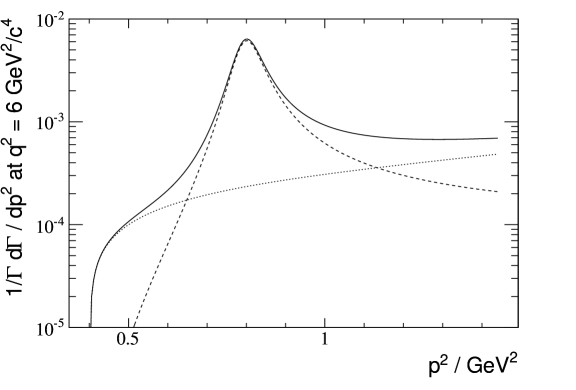
Figure 1: An illustration of the $p^{2}$ spectrum for the P-wave (dashed) and the S-wave (dash-dotted). The total distribution from both states is the solid line. The values were calculated at $q^{2}=6\mathrm{\,Ge\kern-1.00006ptV}^{2}$ by integrating out the angular distribution of $B^{0}\!\rightarrow K^{+}\pi^{-}\ell^{+}\ell^{-}$ using equal matrix elements for each state. The S-wave fraction here is 16% between $800<p<1000\mathrm{\,Me\kern-1.00006ptV}$ 

where the matrix elements from Refs [4, 6] at a $q^{2}$ value of $6\mathrm{\,Ge\kern-1.00006ptV}^{2}$ are used. Here the S-wave amplitude is assumed to be equivalent to the longitudinal P-wave amplitude. The S-wave fraction in the $800<p<1000\mathrm{\,Me\kern-1.00006ptV}$ window around around the P-wave is calculated to be 16% when using this approximation. As will be seen later there are no interference terms left in the angular distribution after the integral over $\cos{\theta_{K}}$.

4 The effect on $B^{0}\!\rightarrow K^{+}\pi^{-}\ell^{+}\ell^{-}$ observables

So far the forward-backward asymmetry ($A_{\mathrm{FB}}$), the fraction of the $K^{*0}$ longitudinal polarisation ($F_{\mathrm{L}}$) and two combinations of the transverse amplitudes ($A_{\mathrm{T}}^{2}$ and $A_{\mathrm{Im}}$) have been measured. As such, these are the observables that will be concentrated on here.

$A_{\mathrm{FB}}$ is defined in terms of the amplitudes as

$$A_{\mathrm{FB}}(q^{2}) =\frac{3}{2}\frac{\Re(A_{1L||}A_{1L\bot}^{*})-\Re(A_{1R||}A_{1R\bot}^{*})}{|A_{10}|^{2}+|A_{1||}|^{2}+|A_{1\bot}|^{2}}$$ (4.1)

for a pure P-wave state where the generic combination of amplitudes $A_{Ji}A_{Ji}^{*}$ is defined as

$$A_{Ji}A_{Ji}^{*} =A_{JiL}A_{JiL}^{*}+A_{JiR}A_{JiR}^{*}.$$ (4.2)

where $i\in\{0,||,\bot,t\}$ and $J=0,1$. The factorisation of the amplitudes into matrix elements and the propagators removes the $p^{2}$ dependence from the theoretical observables. In a similar way, $F_{\mathrm{L}}$, $A_{\mathrm{T}}^{2}$ and $A_{\mathrm{Im}}$ are defined as

$$\begin{split}F_{\mathrm{L}}(q^{2})&=\frac{|A_{10}|^{2}}{|A_{10}|^{2}+|A_{1||}|^{2}+|A_{1\bot}|^{2}},\\ A_{\mathrm{T}}^{2}(q^{2})&=\frac{|A_{1\bot}|^{2}-|A_{1||}|^{2}}{|A_{1\bot}|^{2}+|A_{1||}|^{2}}=(1-F_{\mathrm{L}})\frac{|A_{1\bot}|^{2}-|A_{1||}|^{2}}{|A_{10}|^{2}+|A_{1||}|^{2}+|A_{1\bot}|^{2}},\\ A_{\mathrm{Im}}(q^{2})&=\frac{\Im(A_{1L||}A_{1L\bot}^{*})+\Im(A_{1R||}A_{1R\bot}^{*})}{|A_{10}|^{2}+|A_{1||}|^{2}+|A_{1\bot}|^{2}}.\end{split}$$ (4.3)

These theoretical observables are normalised to the sum of the spin-1 amplitudes. In terms of the angular distribution, $A_{\mathrm{FB}}$ can also be expressed as the difference between the number of ‘forward-going’ $\mu^{+}$ and the number of ‘backward-going’ $\mu^{+}$ in the rest frame of the $B^{0}$,

$$\left[\int_{0}^{1}-\int_{-1}^{0}\right]\text{d}\cos{\theta_{l}}\frac{\text{d}\Gamma}{\text{d}q^{2}\text{d}\cos{\theta_{l}}}/\frac{\text{d}\Gamma}{\text{d}q^{2}}$$ (4.4)

which explains the name of the observable. In Ref [24], this expression was used to determine the zero-crossing point of $A_{\mathrm{FB}}$. The inclusion of the S-wave in the complete angular distribution means that $A_{\mathrm{FB}}$ can no longer be determined by experimentally counting the number of events with forward-going and backward-going leptons, as Eqs. 4.1 and 4.4 are no longer equivalent. However, as the S-wave has no forward-backward asymmetry, no bias occurs in the determination of the zero-crossing point by ignoring the S-wave. The total normalisation for the angular distribution changes to the sum of S- and P-wave amplitudes,

$$\Gamma^{{}^{\prime\prime}} \equiv\frac{\mathrm{d}^{2}\Gamma}{\mathrm{d}p^{2}\mathrm{d}q^{2}}=|A_{10}|^{2}+|A_{1||}|^{2}+|A_{1\bot}|^{2}+|A_{00}|^{2}.$$ (4.5)

such that there is a factor of

$$\mathcal{F}_{\mathrm{P}}(p^{2},q^{2}) =\left(\frac{|A_{10}|^{2}+|A_{1||}|^{2}+|A_{1\bot}|^{2}}{|A_{10}|^{2}+|A_{1||}|^{2}+|A_{1\bot}|^{2}+|A_{00}|^{2}}\right)$$ (4.6)

between the pure P-wave and the admixture of the S and the P-wave. This is the fraction of the yield coming from the P-wave at a given value of $p^{2}$ and $q^{2}$. Similarly, the S-wave fraction is defined as

$$\mathcal{F}_{\mathrm{S}}(p^{2},q^{2}) =\left(\frac{|A_{00}|^{2}}{|A_{10}|^{2}+|A_{1||}|^{2}+|A_{1\bot}|^{2}+|A_{00}|^{2}}\right)$$ (4.7)

and the interference between the S-wave and the P-wave as

$$\mathcal{A}_{\mathrm{S}}(p^{2},q^{2}) =\frac{\sqrt{3}}{2}\left(\frac{|A_{0L0}||A_{1L0}|\cos\delta_{L}+(L\rightarrow R)}{|A_{10}|^{2}+|A_{1||}|^{2}+|A_{1\bot}|^{2}+|A_{00}|^{2}}\right)$$ (4.8)

Substituting the above observables into the angular terms gives

$$\frac{I_{1}^{c}}{\Gamma^{{}^{\prime\prime}}} =\frac{1}{4\pi}\mathcal{F}_{\mathrm{S}}+\frac{3}{4\pi}\mathcal{F}_{\mathrm{P}}F_{\mathrm{L}}\cos^{2}{\theta_{K}}+\frac{3}{4\pi}\mathcal{A}_{\mathrm{S}}\cos{\theta_{K}},$$

$$\frac{I_{1}^{s}}{\Gamma^{{}^{\prime\prime}}} =\frac{3}{4}\frac{3}{8\pi}\mathcal{F}_{\mathrm{P}}\left(1-F_{\mathrm{L}}\right)\left(1-\cos^{2}{\theta_{K}}\right),$$

$$\frac{I_{2}^{c}}{\Gamma^{{}^{\prime\prime}}} =-\left(\frac{1}{4\pi}\right.\mathcal{F}_{\mathrm{S}}+\frac{3}{4\pi}\mathcal{F}_{\mathrm{P}}\left(1-F_{\mathrm{L}}\right)\cos^{2}{\theta_{K}}+\left.\frac{3}{4\pi}\mathcal{A}_{\mathrm{S}}\cos{\theta_{K}}\cos{\theta_{K}}\right),$$

$$\frac{I_{2}^{s}}{\Gamma^{{}^{\prime\prime}}} =\frac{1}{4}\frac{3}{8\pi}\mathcal{F}_{\mathrm{P}}\left(1-F_{\mathrm{L}}\right)\left(1-\cos^{2}{\theta_{K}}\right),$$ (4.9)

$$\frac{I_{3}}{\Gamma^{{}^{\prime\prime}}} =\frac{1}{2}\frac{3}{8\pi}\mathcal{F}_{\mathrm{P}}A_{\mathrm{T}}^{2}\left(1-\cos^{2}{\theta_{K}}\right),$$

$$\frac{I_{6}}{\Gamma^{{}^{\prime\prime}}} =2\frac{3}{8\pi}\frac{4}{3}\mathcal{F}_{\mathrm{P}}A_{\mathrm{FB}}\left(1-\cos^{2}{\theta_{K}}\right),$$

$$\frac{I_{9}}{\Gamma^{{}^{\prime\prime}}} =\frac{3}{8\pi}\mathcal{F}_{\mathrm{P}}A_{\mathrm{Im}}\left(1-\cos^{2}{\theta_{K}}\right).$$

For the purpose of this paper, a simplification of the angular distribution can be achieved by folding the distribution in $\phi$ such that $\phi^{{}^{\prime}}=\phi-\pi$ for $\phi<0$ [27]. The $I_{4,5,7,8}$ angular terms which are dependent on $\cos\phi$ or $\sin\phi$ are cancelled leaving $I_{1,2,3,6,9}$ in the angular distribution:

$$\frac{\text{d}^{5}\Gamma}{\text{d}q^{2}\text{d}p^{2}\mathrm{dcos}{\theta_{K}}\mathrm{dcos}{\theta_{l}}\text{d}\phi^{{}^{\prime}}}= \frac{3}{8}\left(I_{1}^{c}+2I_{1}^{s}+(I_{2}^{c}+2I_{2}^{s})\cos 2\theta_{l}+2I_{3}\sin^{2}{\theta_{l}}\cos 2\phi^{{}^{\prime}}\right.$$

$$\left.+2I_{6}\cos{\theta_{l}}+2\sqrt{2}I_{9}\sin^{2}{\theta_{l}}\sin 2\phi^{{}^{\prime}}\frac{}{}\right).$$ (4.10)

Combining Equation 4 with 4 gives the differential decay distribution,

$$\begin{split}\frac{1}{\Gamma^{{}^{\prime\prime}}}\frac{\text{d}^{5}\Gamma}{\text{d}q^{2}\text{d}p^{2}\mathrm{dcos}{\theta_{K}}\mathrm{dcos}{\theta_{l}}\text{d}\phi^{{}^{\prime}}}=\frac{9}{16\pi}\Bigg{(}&\left(\frac{2}{3}\mathcal{F}_{\mathrm{S}}+\frac{4}{3}\mathcal{A}_{\mathrm{S}}\cos{\theta_{K}}\right)(1-\cos^{2}{\theta_{l}})\\ &\ \ \ \ +\mathcal{F}_{\mathrm{P}}\bigg{[}2F_{\mathrm{L}}\cos^{2}{\theta_{K}}(1-\cos^{2}{\theta_{l}})\\ &\ \ \ \ \ \ \ \ +\frac{1}{2}(1-F_{\mathrm{L}})(1-\cos^{2}{\theta_{K}})(1+\cos^{2}{\theta_{l}})\\ &\ \ \ \ \ \ \ \ +\frac{1}{2}(1-F_{\mathrm{L}})A_{\mathrm{T}}^{2}(1-\cos^{2}{\theta_{K}})(1-\cos^{2}{\theta_{l}})\cos 2\phi^{{}^{\prime}}\\ &\ \ \ \ \ \ \ \ +\frac{4}{3}A_{\mathrm{FB}}(1-\cos^{2}{\theta_{K}})\cos{\theta_{l}}\\ &\ \ \ \ \ \ \ \ +A_{\mathrm{Im}}(1-\cos^{2}{\theta_{K}})(1-\cos^{2}{\theta_{l}})\sin 2\phi^{{}^{\prime}}\bigg{]}\Bigg{)}.\end{split}$$ (4.11)

The angular distribution as a function of $\cos{\theta_{l}}$ and $\cos{\theta_{K}}$ is given by integrating over $\phi$ in Eq. 4.11

$$\begin{split}\frac{1}{\Gamma^{{}^{\prime\prime}}}\frac{\text{d}^{4}\Gamma}{\text{d}q^{2}\text{d}p^{2}\text{d}\cos{\theta_{K}}\text{d}\cos{\theta_{l}}}=\frac{9}{16}&\Bigg{(}\left(\frac{2}{3}\mathcal{F}_{\mathrm{S}}+\frac{4}{3}\mathcal{A}_{\mathrm{S}}\cos{\theta_{K}}\right)(1-\cos^{2}{\theta_{l}})\\ &+\mathcal{F}_{\mathrm{P}}\bigg{[}2F_{\mathrm{L}}\cos^{2}{\theta_{K}}(1-\cos^{2}{\theta_{l}})\\ &\ \ \ \ \ +\frac{1}{2}(1-F_{\mathrm{L}})(1-\cos^{2}{\theta_{K}})(1+\cos^{2}{\theta_{l}})\\ &\ \ \ \ \ +\frac{4}{3}A_{\mathrm{FB}}(1-\cos^{2}{\theta_{K}})\cos{\theta_{l}}\bigg{]}\Bigg{)}\end{split}$$ (4.12)

and further integration from Equation 4.11 yields the angular distribution for each of the angles,

$$\begin{split}\frac{1}{\Gamma^{{}^{\prime\prime}}}\frac{\text{d}^{3}\Gamma}{\text{d}q^{2}\text{d}p^{2}\mathrm{dcos}{\theta_{l}}}&=\frac{3}{4}\mathcal{F}_{\mathrm{S}}(1-\cos^{2}{\theta_{l}})+\mathcal{F}_{\mathrm{P}}\bigg{[}\frac{3}{4}F_{\mathrm{L}}(1-\cos^{2}{\theta_{l}})\\ &+\frac{3}{8}(1-F_{\mathrm{L}})(1+\cos^{2}{\theta_{l}})+A_{\mathrm{FB}}\cos{\theta_{l}}\bigg{]},\\ \frac{1}{\Gamma^{{}^{\prime\prime}}}\frac{\text{d}^{3}\Gamma}{\text{d}q^{2}\text{d}p^{2}\mathrm{dcos}{\theta_{K}}}&=\frac{1}{2}\mathcal{F}_{\mathrm{S}}+\mathcal{A}_{\mathrm{S}}\cos{\theta_{K}}\\ &+\mathcal{F}_{\mathrm{P}}\bigg{[}\frac{3}{2}F_{\mathrm{L}}\cos^{2}{\theta_{K}}+\frac{3}{4}(1-F_{\mathrm{L}})(1-\cos^{2}{\theta_{K}})\bigg{]},\\ \frac{1}{\Gamma^{{}^{\prime\prime}}}\frac{\text{d}^{3}\Gamma}{\text{d}q^{2}\text{d}p^{2}\text{d}\phi^{{}^{\prime}}}&=\frac{1}{\pi}\Bigg{(}1+\frac{3}{4}\mathcal{F}_{\mathrm{S}}+\mathcal{F}_{\mathrm{P}}\bigg{[}F_{\mathrm{L}}+\frac{1}{2}(1-F_{\mathrm{L}})A_{\mathrm{T}}^{2}\cos 2\phi^{{}^{\prime}}+A_{\mathrm{Im}}\sin 2\phi^{{}^{\prime}}\bigg{]}\Bigg{)}.\end{split}$$ (4.13)

The angular distribution can be integrated over $p^{2}$ using the weighted integral

$$O(q^{2}) =\frac{\int\mathcal{O}(p^{2},q^{2})\frac{\text{d}^{2}\Gamma}{\text{d}p^{2}\text{d}q^{2}}\text{d}p^{2}}{\int\frac{\text{d}^{2}\Gamma}{\text{d}p^{2}\text{d}q^{2}}\text{d}p^{2}}$$ (4.14)

for the value of the observables integrated over a given region in $p^{2}$. This leads to the integrated observables $F_{\mathrm{P}}$, $F_{\mathrm{S}}$ and $A_{\mathrm{S}}$ which are solely dependant on $q^{2}$. By definition, the fraction of the S-wave and the P-wave sum to one, $F_{\mathrm{S}}+F_{\mathrm{P}}=1$. The complete angular distribution without any $p^{2}$ dependence is given by

$$\frac{1}{\Gamma^{{}^{\prime}}}\frac{\text{d}^{5}\Gamma}{\text{d}q^{2}\mathrm{dcos}{\theta_{K}}\mathrm{dcos}{\theta_{l}}\text{d}\phi^{{}^{\prime}}}=\frac{9}{16\pi} \Bigg{(}\left(\frac{2}{3}F_{\mathrm{S}}+\frac{4}{3}A_{\mathrm{S}}\cos{\theta_{K}}\right)(1-\cos^{2}{\theta_{l}})$$

$$+(1-F_{\mathrm{S}})\bigg{[}2F_{\mathrm{L}}\cos^{2}{\theta_{K}}(1-\cos^{2}{\theta_{l}})$$

$$\ \ \ \ \ \ \ \ \ \ \ \ +\frac{1}{2}(1-F_{\mathrm{L}})(1-\cos^{2}{\theta_{K}})(1+\cos^{2}{\theta_{l}})$$

$$\ \ \ \ \ \ \ \ \ \ \ \ +\frac{1}{2}(1-F_{\mathrm{L}})A_{\mathrm{T}}^{2}(1-\cos^{2}{\theta_{K}})(1-\cos^{2}{\theta_{l}})\cos 2\phi^{{}^{\prime}}$$

$$\ \ \ \ \ \ \ \ \ \ \ \ +\frac{4}{3}A_{\mathrm{FB}}(1-\cos^{2}{\theta_{K}})\cos{\theta_{l}}$$

$$\ \ \ \ \ \ \ \ \ \ \ \ +A_{\mathrm{Im}}(1-\cos^{2}{\theta_{K}})(1-\cos^{2}{\theta_{l}})\sin 2\phi^{{}^{\prime}}\bigg{]}\Bigg{)}.$$ (4.15)

where the normalisation of the angular distribution is given by

$$\Gamma^{{}^{\prime}}=\frac{\mathrm{d}\Gamma}{\mathrm{d}q^{2}}$$ (4.16)

The ‘dilution’ effect of the S-wave can clearly be seen from the factor of (1-$F_{\mathrm{S}}$) that appears in front of the observables in Eq. 4.

The effect of an S-wave on the angular distribution as a function of $\cos{\theta_{K}}$, $\cos{\theta_{l}}$ and $\phi^{{}^{\prime}}$ as illustrated in Figure 2.

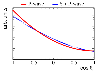
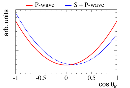
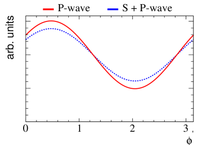
Figure 2: One-dimensional projections of (a) $\cos{\theta_{l}}$, (b) $\cos{\theta_{K}}$, (c) $\phi^{{}^{\prime}}$ for the angular distribution of $B^{0}\!\rightarrow K^{*0}\ell^{+}\ell^{-}$ with (blue-dashed) and without (red-solid) an S-wave component of 7%. The dilution effect of the S-wave on the asymmetry in $\cos{\theta_{l}}$ and the asymmetric effect in $\cos{\theta_{K}}$ can be clearly seen. 

Here it is possible to see that the asymmetry in $\cos{\theta_{l}}$, given by $A_{\mathrm{FB}}$, has decreased and that there is an asymmetry in $\cos{\theta_{K}}$ introduced by the interference term.

5 Effect of an S-wave on the angular analysis

In an angular analysis of $B^{0}\!\rightarrow K^{+}\pi^{-}\ell^{+}\ell^{-}$, the S-wave can be considered to be a systematic effect that could bias the results of the angular observables. The implications of this systematic effect are tested by generating toy Monte Carlo experiments and fitting the angular distribution to them. The results of the fit to the observables are evaluated for multiple toy datasets.

The effect of the S-wave is evaluated for two different cases. Firstly, the effect of S-wave interference is examined as a function of the size of the dataset used. The aim of this is to give an idea of the current situation and the possible implications on future measurements of $B^{0}\!\rightarrow K^{+}\pi^{-}\ell^{+}\ell^{-}$. Datasets of sizes between 50 and 1000 events are tested. For comparison, the latest results from LHCb [24] have between 20 and 200 signal events in the 6 different $q^{2}$ bins considered. Secondly, the effect of different levels of S-wave contribution is examined. At present, the only information about the S-wave fraction is the measurement of $F_{\mathrm{S}}$ of approximately 7% in the decay $B^{0}\rightarrow{J\mskip-3.0mu/\mskip-2.0mu\psi\mskip 2.0mu}K^{+}\pi^{-}$ from [15] for the range $800<p<1000\mathrm{\,Me\kern-1.00006ptV}$. As the value may be different in $B^{0}\!\rightarrow K^{+}\pi^{-}\ell^{+}\ell^{-}$, we consider values of $F_{\mathrm{S}}$ in this region ranging from 1% to 40%. The fraction of the S-wave, $F_{\mathrm{S}}$, is expected to have some $q^{2}$ dependence because of the $q^{2}$ dependence of the transverse P-wave amplitudes.

The parameters used to generate the toy datasets are summarised in Tables 1 and 2. The values of the angular observables used to generate toy Monte Carlo simulations are taken from the LHCb angular analysis of $B^{0}\!\rightarrow K^{*0}\mu^{+}\mu^{-}$ in the $1<q^{2}<6\mathrm{\,Ge\kern-1.00006ptV}^{2}$ bin [24]. Within errors, these measurements are compatible with the Standard Model prediction for $B^{0}\!\rightarrow K^{*0}\ell^{+}\ell^{-}$ and the central value of the measurement is used. The nominal magnitude and phase difference of the S-wave contribution are taken from the angular analysis of $B^{0}$ $\rightarrow$ ${J\mskip-3.0mu/\mskip-2.0mu\psi\mskip 2.0mu}$ $K^{+}\pi^{-}$ [15].

Table 2: Parameters used to generate toy datasets. $A_{\mathrm{FB}}$, $F_{\mathrm{L}}$, $A_{\mathrm{T}}^{2}$ and $A_{\mathrm{Im}}$ are taken from Ref. [24] in the $1<q^{2}<6~{}(\mathrm{\,Ge\kern-1.00006ptV}^{2})$ bin. The $F_{\mathrm{S}}$ value is taken from Ref. [15] 

. Obs. $A_{\mathrm{FB}}$ $F_{\mathrm{L}}$ $A_{\mathrm{T}}^{2}$ $A_{\mathrm{Im}}$ $F_{\mathrm{S}}$ Value $-0.18$ $0.66$ $0.294$ $0.07$ $0.07$

The toy datasets are generated as a function of the $\cos{\theta_{l}}$, $\cos{\theta_{K}}$, $\phi$ and $p^{2}$ using the angular distribution given in Eq. 4.11. For each set of input parameters 1000 toy datasets were generated. For each of these toy datasets, an unbinned log likelihood fit is performed that returns the best fit value of the observables and an estimate of their error. The expected experimental resolution is obtained by plotting the best fit values of an observable for the ensemble of toy simulations as illustrated for $A_{\mathrm{FB}}$ in Fig. 3 (left) The pull value for an observable ($O$) is defined as

$$p_{O}^{i}=\frac{O_{\text{fit}}^{i}-O_{\text{gen}}^{i}}{\sigma_{O}^{i}}$$ (5.1)

where $\sigma_{O}^{i}$ is the estimated error on the fit to the observable $O^{i}$. This distribution is seen in Fig. 3 (right). The mean and the width are extracted from a Gaussian fit. For a well performing fit without bias, the pull distribution should have zero mean and unit width. A negative pull value implies that the result is underestimated and a positive pull value implies overestimation of the true observable.

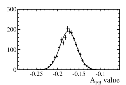
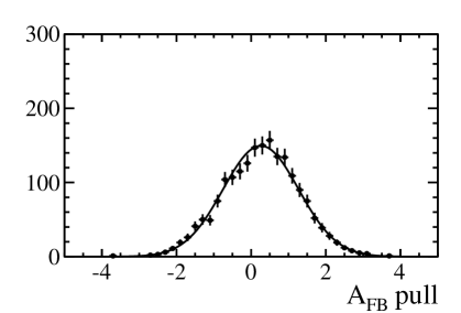
Figure 3: Distribution of (left) the $A_{\mathrm{FB}}$ results and (right) pull values for fits to 1000 toy simulations each containing 1000 events. The S-wave is ignored in these fits. The resolution obtained is $(0.026\pm 0.001)$. Since the S-wave is ignored there is a non-zero pull mean at $(0.26\pm 0.02)\sigma$ . The width of the pull distribution is consistent with unity at $(1.01\pm 0.01)\sigma$. 

5.1 The impact of ignoring the S-wave in an angular analysis of $B^{0}\!\rightarrow K^{*0}\ell^{+}\ell^{-}$

Firstly, the effect of an S-wave was tested as a function of dataset size in order to find a minimum dataset at which the bias from the S-wave in the angular observables becomes significant. Datasets were generated for sample sizes ranging from 50 and 1000 events and analysed assuming a pure P-wave state. The results are shown in Fig. 4.

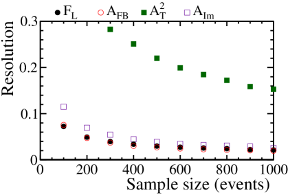
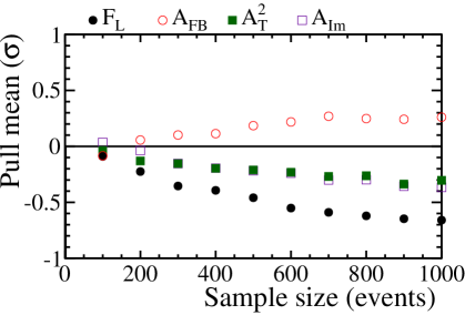
Figure 4: Resolution (left) and pull mean (right) of 1000 toy datasets analysed as a pure P-wave state as a function of dataset size. It can be seen that the bias on the observable increases dramatically as the sample size increases. This is because the statistical error decreases increasing the sensitivity to the S-wave contribution. The bias of $A_{\mathrm{FB}}$ is positive because $A_{\mathrm{FB}}$ in negative in the $q^{2}$ bin chosen.  

From Eq. 4.12, it can be seen that $A_{\mathrm{T}}^{2}$ has a factor of (1-$F_{\mathrm{L}}$) in front of it. The large value of $F_{\mathrm{L}}$ used in generated the datasets is in turn causing $A_{\mathrm{T}}^{2}$ to have a much worse resolution than $A_{\mathrm{FB}}$, $F_{\mathrm{L}}$ and $A_{\mathrm{Im}}$. There is significant bias (non-zero mean) of the pull distribution for all observables when the S-wave is ignored for datasets of more than 200 events. This corresponds to a change of 0.2$\sigma$ in $F_{\mathrm{L}}$ for a dataset of 200 events. The behaviour can be understood in terms of the $(1-F_{\mathrm{S}})$ factor in Eq 4.12. It gives an offset to the fitted value of the observables which are proportional to the value of $F_{\mathrm{S}}$.

Secondly, the angular fit was performed on toy datasets with an increasing S-wave contribution. Datasets of 500 events were generated with a varying S-wave contribution in the narrow $p^{2}$ mass window of ($800<p<1000\mathrm{\,Me\kern-1.00006ptV}$) from no S-wave up to a $F_{\mathrm{S}}$ value of $0.6$. The resolution, the mean and width of the pull distribution for each of the four observables ($A_{\mathrm{FB}}$, $F_{\mathrm{L}}$, $A_{\mathrm{T}}^{2}$, $A_{\mathrm{Im}}$) were calculated and the results are shown in Fig. 5.

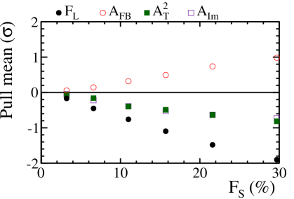
Figure 5: Mean of the pull distribution of 1000 toy datasets analysed as a pure P-wave state as a function of S-wave contribution. The bias can be seen to increase with the size of the S-wave contribution in a linear fashion.  

Significant bias is seen in the angular observable for an S-wave magnitude of greater than 5%. The linear increase in the bias is another consequence of the (1-$F_{\mathrm{S}}$) factor.

5.2 Measuring the S-wave in $B^{0}\!\rightarrow K^{+}\pi^{-}\ell^{+}\ell^{-}$

Obtaining unbiased values for the angular observables beyond the limits shown requires a measurement of the S-wave contribution rather than ignoring it. With the formalism developed in Sect.4, three options are explored for measuring this. The first option is to ignore the $p^{2}$ dependence and simply fit for $p^{2}$-averaged values of $F_{\mathrm{S}}$ and $A_{\mathrm{S}}$. The second option is to fit the $p^{2}$ line-shape simultaneously with the angular distribution. This can be done in a small $p$ window between $800$ and $1000\mathrm{\,Me\kern-1.00006ptV}$ or in the region from the lower kinematic threshold to $1200\mathrm{\,Me\kern-1.00006ptV}$. In all cases the datasets used to perform the studies are identical to those used in Sect. 5.1. The difference is in how the fit is performed. In each case, the dataset and the S-wave sizes refer to the number of events in the smaller $p^{2}$ window.

The angular distribution without $p^{2}$ dependence is given in Eq. 4. for each set of samples, we look at the resolution, the mean and the width of the pull distribution of the angular observables.

The change in the resolution obtained on the angular observables for the three methods of including the S-wave in the angular distribution is demonstrated by plotting the ratio with respect to the resolution obtained when a single P-wave state is assumed.

The resolutions and the mean of the pull distributions for the three different fit methods (ignoring the $p^{2}$ dependence, fitting a narrow $p^{2}$ window and fitting a wide $p^{2}$ window) relative to the resolution and mean obtained using the assumption of a pure P-wave state. The ratio between the fit methods including the S-wave in angular distribution and assuming a P-wave state as a function of dataset size are shown in Fig 6.

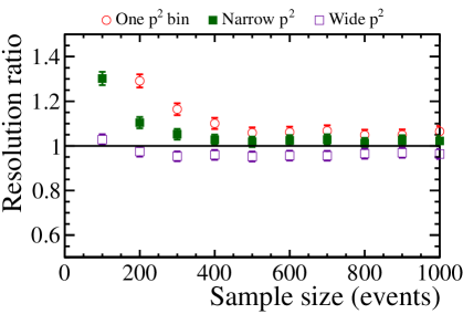
(a) $A_{\mathrm{FB}}$

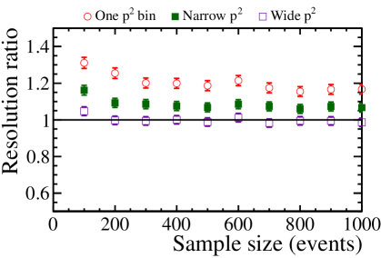
(b) $F_{\mathrm{L}}$

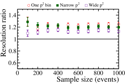
(c) $A_{\mathrm{T}}^{2}$

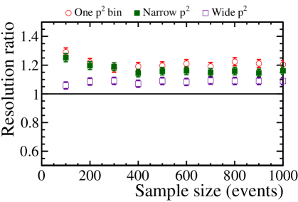
(d) $A_{\mathrm{Im}}$

Figure 6: Resolutions for three different methods to incorporate the S-wave relative to the resolution obtained when the S-wave is ignored. It can be seen that the best resolution is obtained when using the largest $p^{2}$ window. The original resolution is recovered to within 10%.  

The pull mean for all four fit methods is shown in Fig 7.

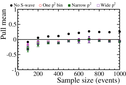
(a) $A_{\mathrm{FB}}$

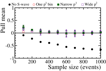
(b) $F_{\mathrm{L}}$

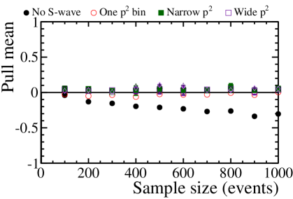
(c) $A_{\mathrm{T}}^{2}$

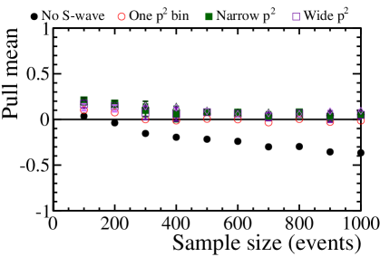
(d) $A_{\mathrm{Im}}$

Figure 7: Pull mean for the three different methods to incorporate the S-wave and when the S-wave is ignored. There is a slight bias when the S-wave is included for datasets of less than 200 events but this bias is removed from all the observables when the S-wave is included in the fit for datasets of over 500 events.  

For all observables, it can be seen that the resolution degrades when the S-wave is included and the $p^{2}$ dependence is ignored. The resolution degrades by a smaller amount when the $p^{2}$ dependence is included in a small bin and the original resolution is recovered to within 10% when using the large $p^{2}$ range. There are two effects contributing to the improvement of the resolution. There are more P-wave events in the larger range and the wider mass window allows for the S-wave to be constrained by using the information from above and below the P-wave resonance. This results in the best resolution when the S-wave is included in the angular distribution.

For all the observables, the pull mean approaches zero for datasets of greater than 300 events implying that the bias present in all the observables when a pure P-wave state is removed when an S-wave is included in the angular distribution. This means that the inclusion of the S-wave component will be mandatory for all future experimental analyses.

Another approach to reduce the bias from the S-wave is to ignore it in fits but to only include data from a narrower window in $p$ arounnd the $K^{*0}(892)$ resonance. By reducing the window from 200$\mathrm{\,Me\kern-1.00006ptV}$ to 100$\mathrm{\,Me\kern-1.00006ptV}$, the P-wave component is reduced by 20% while the S-wave component is roughly halved. Conducting the same tests as described above shows, as expected, a 10% increase in the statistical error of the observables while the bias for a given dataset is reduced by a factor two. Given what has been shown in this paper, the experimental datasets will in the future be so large that the best approach is to fit the S-wave rather than half the bias and accepting an increased statistical uncertainty.

Until now the lineshape of the S-wave has been parameterised according to the LASS model (Eqs. 3.7-3.9). We asses the model dependence of this assumption by using the alternative isobar model [28] for generating the S-wave component while keeping the same fit model. This only has an effect on the fits where a fit is performed to the $p^{2}$ dependence. The results of this show that the systematic uncertainly due to the model dependence is much smaller than the statistical error for all observables for all sample sizes we studied.

6 Conclusion

In summary, the inclusion of a resonant $K^{+}\pi^{-}$ S-wave in the angular analysis of $B^{0}\!\rightarrow K^{*0}\ell^{+}\ell^{-}$ has been formalised and the complete angular distribution for both an S- and P-wave state described. We find that the inclusion of an S-wave state has an overall dilution effect on the theoretical observables. The impact of an S-wave on an angular analysis is evaluated using toy Monte Carlo datasets. We find that the S-wave contribution can only be ignored for datasets of less than 200 events. The bias on the angular observables incurred by assuming a pure P-wave $K^{+}\pi^{-}$ state can be removed by including the S-wave in the angular distribution. The degradation in resolution on the angular observables from fitting a more complicated angular distribution can be minimised by performing the fit in a wide region around the $K^{*0}(892)$ resonance. The systematic uncertainty introduced by the model dependence of the S-wave lineshape is minimal and can be ignored.

References

- [1] Heavy Flavor Averaging Group, D. Asner et al., Averages of b-hadron, c-hadron, and -lepton properties, arXiv:1010.1589
- [2] Krüger, F. and Sehgal, L. M. and Sinha, N. and Sinha, R., Angular distribution and CP asymmetries in the decays and , Phys. Rev. D61 (2000) 114028
- [3] Kruger, F. and Matias, J., Probing new physics via the transverse amplitudes of at large recoil, Phys. Rev. D71 (2005) 094009, arXiv:hep-ph/0502060
- [4] U. Egede et al., New observables in the decay mode , JHEP 11 (2008) 032, arXiv:0807.2589
- [5] W. Altmannshofer et al., Symmetries and asymmetries of decays in the standard model and beyond, JHEP 01 (2009) 019, arXiv:0811.1214
- [6] U. Egede et al., New physics reach of the decay mode , JHEP 10 (2010) 056, arXiv:1005.0571
- [7] C. Bobeth, G. Hiller, and D. van Dyk, The benefits of decays at low recoil, JHEP 07 (2010) 098, arXiv:1006.5013
- [8] J. Matias, F. Mescia, M. Ramon, and J. Virto, Complete anatomy of and its angular distribution, JHEP 04 (2012) 104, arXiv:1202.4266
- [9] BaBar collaboration, B. Aubert et al., Angular distributions in the decays , Phys. Rev. D79 (2009) 031102, arXiv:0804.4412
- [10] Belle collaboration, J.-T. Wei et al., Measurement of the differential branching fraction and forward-backward asymmetry for , Phys. Rev. Lett. 103 (2009) 171801, arXiv:0904.0770
- [11] CDF collaboration, T. Aaltonen et al., Measurement of the forward-backward asymmetry in the decay and first observation of the decay, Phys. Rev. Lett. 106 (2011) 161801, arXiv:1101.1028
- [12] LHCb collaboration, R. Aaij et al., Differential branching fraction and angular analysis of the decay , Phys. Rev. Lett. 108 (2012) 181806, arXiv:1112.3515
- [13] Particle Data Group, J. Beringer et al., Review of Particle Physics (RPP), Phys. Rev. D86 (2012) 010001
- [14] LASS collaboration, D. Aston et al., A study of scattering in the reaction p n at 11 / c, Nucl. Phys. B296 (1987) 493.
- [15] BaBar collaboration, B. Aubert et al., Ambiguity-free measurement of : time-integrated and time-dependent angular analyses of , Phys. Rev. D71 (2005) 032005, arXiv:hep-ex/0411016
- [16] LHCb collaboration, R. Aaij et al., Determination of the sign of the decay width difference in the system, Phys. Rev. Lett. 108 (2012) 241801, arXiv:1202.4717
- [17] Y. Xie, P. Clarke, G. Cowan, and F. Muheim, Determination of 2 in decays in the presence of a K+ K- S-wave contribution, JHEP 09 (2009) 074, arXiv:0908.3627
- [18] CDF collaboration, T. Aaltonen et al., Measurement of the CP-violating phase in decays with the CDF II Detector, Phys. Rev. D85 (2012) 072002, arXiv:1112.1726
- [19] D0 collaboration, V. M. Abazov et al., Measurement of the CP-violating phase using the flavor-tagged decay in 8 fb-1 of collisions, Phys. Rev. D85 (2012) 032006, arXiv:1109.3166
- [20] LHCb collaboration, R. Aaij et al., Measurement of the CP-violating phase in the decay , Phys. Rev. Lett. 108 (2012) 101803, arXiv:1112.3183
- [21] D. Becirevic and A. Tayduganov, Impact of on the New Physics search in decay, arXiv:1207.4004
- [22] J. Matias, On the S-wave pollution of observables, Phys. Rev. D86 (2012) 094024, arXiv:1209.1525
- [23] C.-D. Lu and W. Wang, Analysis of in the higher kaon resonance region, Phys. Rev. D85 (2012) 034014, arXiv:1111.1513
- [24] LHCb collaboration, Differential branching fraction and angular analysis of the decay, LHCb-CONF-2012-008
- [25] J. M. Blatt and V. F. Weisskopf, Theoretical nuclear physics, Springer, New York, NY, 1979
- [26] BaBar collaboration, B. Aubert et al., Search for the at BABAR, Phys. Rev. D79 (2009) 112001, arXiv:0811.0564
- [27] J. Lefrancois and M. H. Schune, Measuring the photon polarization in using the decay channel, LHCb-PUB-2009-008
- [28] E791 collaboration, E. M. Aitala et al., Dalitz plot analysis of the decay and indication of a low-mass scalar resonance, Phys. Rev. Lett. 89 (2002) 121801