Bayesian Conditional Monte Carlo Algorithms for Sequential Single and Multi-Object filtering

Abstract

Bayesian filtering aims at tracking sequentially a hidden process from an observed one. In particular, sequential Monte Carlo (SMC) techniques propagate in time weighted trajectories which represent the posterior probability density function (pdf) of the hidden process given the available observations. On the other hand, Conditional Monte Carlo (CMC) is a variance reduction technique which replaces the estimator of a moment of interest by its conditional expectation given another variable. In this paper we show that up to some adaptations, one can make use of the time recursive nature of SMC algorithms in order to propose natural temporal CMC estimators of some point estimates of the hidden process, which outperform the associated crude Monte Carlo (MC) estimator whatever the number of samples. We next show that our Bayesian CMC estimators can be computed exactly, or approximated efficiently, in some hidden Markov chain (HMC) models; in some jump Markov state-space systems (JMSS); as well as in multitarget filtering. Finally our algorithms are validated via simulations.

1 Introduction

1.1 SMC algorithms for single- or multi-object Bayesian filtering

In single object Bayesian filtering we consider two random processes $\{X_{n}\}_{n\geq 0}$ and $\{Y_{n}\}_{n\geq 0}$ with given joint probability law. $Y_{i}$ is observed, i.e. we have at our disposal realizations ${\bf y}_{0:n}=\{y_{i}\}_{i=0}^{n}$ of ${\bf Y}_{0:n}=\{Y_{i}\}_{i=0}^{n}$ (as far as notations are concerned, upper case letters denote random variables (r.v.), lower case ones their realizations, and bold letters vectors; $p(x)$, say, denotes the pdf of r.v. $X$ and $p(x|y)$, say, the conditional pdf of $X$ given $Y=y$; if $i\leq j$ $p_{i:j|n}$ is a shorthand notation for $p({\bf x}_{i:j}|{\bf y}_{0:n})$; if $x^{i}$ are samples from $p(x)$ then the set $\{x^{i}\}_{i=1}^{N}$ can also be denoted ${\bf x}^{1:N}$; subscripts are reserved for times indices and superscripts for realizations). Process $\{X_{n}\}$ is hidden, and our aim is to compute, for each time instant $n$, some moment of interest

$$\Theta_{n}=\int f({\bf x}_{0:n})p({\bf x}_{0:n}|{\bf y}_{0:n}){\rm d}{\bf x}_{0:n}$$ (1)

of the a posteriori pdf $p({\bf x}_{0:n}|{\bf y}_{0:n})$ of ${\bf X}_{0:n}$ given ${\bf y}_{0:n}$. Unfortunately, in most models (1) cannot be computed exactly. Suboptimal solutions for computing $\Theta_{n}$ include SMC techniques livredoucet arulampalamshort , which propagate over time weighted trajectories $\{{\bf x}_{0:n}^{i},w_{n}^{i}\}_{i=1}^{N}$ with $\sum_{i=1}^{N}w_{n}^{i}=1$. In other words, $\widehat{p}_{0:n|n}=\sum_{i=1}^{N}w_{n}^{i}\delta_{{\bf x}_{0:n}^{i}}$, in which $\delta$ is the Dirac mass, is a discrete (and random) approximation of $p({\bf x}_{0:n}|{\bf y}_{0:n})$.

On the other hand, multi-object filtering (see e.g. MAHLER_ARTICLE2003 ) essentially reduces to computing $\Theta_{n}=\int f({\bf x}_{n})v_{n}({\bf x}_{n}){\rm d}{\bf x}_{n}$ in which $v_{n}({\bf x}_{n})$ is now the so-called Probability Hypothesis Density (PHD), i.e. the a posteriori spatial density of the expected number of targets, given all measurements (be they due to detected targets or to false alarms). Again, SMC techniques propagate an approximation of $v_{n}$ with a set of weighted samples $\{{\bf x}_{n}^{i},w_{n}^{i}\}_{i=1}^{N}$; here $\sum_{i=1}^{N}w_{n}^{i}$, which in general is different from $1$, is an estimator of the number of targets.

Now, SMC algorithms, be they for single- or multi-object Bayesian filtering, usually focus on how to propagate approximations $\widehat{p}_{0:n|n}$ (or $\widehat{v}_{n}$) of ${p}_{0:n|n}$ (or $v_{n}$); once $\widehat{p}_{0:n|n}$ or $\widehat{v}_{n}$ has been computed, $\Theta_{n}$ is finally estimated either as $\widehat{\Theta}_{n}=\sum_{i=1}^{N}w_{n}^{i}f({\bf x}_{0:n}^{i})$ or $\sum_{i=1}^{N}w_{n}^{i}f({\bf x}_{n}^{i})$. By contrast, in this paper we directly focus on $\widehat{\Theta}_{n}$ itself, and see under which conditions one can improve this point estimator at a reasonable computational cost.

1.2 Variance reduction via conditioning: Rao-Blackwellized particle filters (RB-PF)

This problem leads us to variance reduction techniques which form an important part of computer simulation (see e.g. asmussen-glynn ). Among them, methods based on conditioning variables rely on the following well known result. Let $X_{1}$ and $X_{2}$ be two r.v. and $f$ some function. Then

$${\rm E}({\rm E}(f(X_{2})|X_{1})) = {\rm E}(f(X_{2})),$$ (2)

$${\rm var}({\rm E}(f(X_{2})|X_{1})) = {\rm var}(f(X_{2}))-{\rm E}({\rm var}(f(X_{2})|X_{1})).$$ (3)

So if the aim is to compute $\Theta={\rm E}(f(X_{2}))$ and we have at our disposal $\{X_{1}^{i}\}_{i=1}^{N}\stackrel{{\scriptstyle\rm i.i.d.}}{{\sim}}p(x_{1})$, $\{X_{2}^{i}\}_{i=1}^{N}\stackrel{{\scriptstyle\rm i.i.d.}}{{\sim}}p(x_{2})$ then the so-called CMC estimator $\widetilde{\Theta}=\frac{1}{N}\sum_{i=1}^{N}{\rm E}(f(X_{2})|X_{1}^{i})$ has lower variance than the corresponding crude MC one $\widehat{\Theta}=\frac{1}{N}\sum_{i=1}^{N}f(X_{2}^{i}).$ Of course, the interest of $\widetilde{\Theta}$ vs. $\widehat{\Theta}$ depends on the choice of $X_{1}$: ideally, one should easily sample from $p(x_{1})$; the variance reduction in (3) should be as large as possible; but in the meantime function $g(x_{1})={\rm E}(f(X_{2})|x_{1})$ should remain computable at a reasonable computational cost.

Variance reduction techniques based on CMC methods have been adapted to Bayesian filtering; in this context, these methods are either known as marginalized or RB-PF Chen-Mixture-Kalman doucet-sequentialMC doucet-jump-Mkv Shon-MPF . The rationale is as follow. Let now $\Theta_{n}$ in (1) be rewritten as $\Theta={\rm E}(f(X_{1},X_{2}))$. It is usually not possible to sample from $p(x_{1},x_{2})$, and often $p(x_{1},x_{2})\propto p^{\prime}(x_{1},x_{2})$ is only known up to a constant, whence the use of Bayesian (or normalized) importance sampling (IS) techniques Gewecke . So let

$$\widehat{\Theta}({\bf x}_{1}^{1:N},{\bf x}_{2}^{1:N}) =\sum_{i=1}^{N}w_{2}^{i}({\bf x}_{1}^{1:N},{\bf x}_{2}^{1:N})f(x_{1}^{i},x_{2}^{i})\text{ with }(x_{1}^{i},x_{2}^{i})\sim q_{2}\text{,}$$ (4)

$$\widehat{\Theta}^{\rm RB}({\bf x}_{1}^{1:N}) =\sum_{i=1}^{N}w_{1}^{i}({\bf x}_{1}^{1:N}){\rm E}(f(x_{1}^{i},X_{2})|x_{1}^{i})\text{ with }x_{1}^{i}\sim q_{1},$$ (5)

with $\sum_{i=1}^{N}w_{1}^{i}=$ $\sum_{i=1}^{N}w_{2}^{i}=1.$ Estimator $\widehat{\Theta}^{\rm RB}$ depends on samples $\{x_{1}^{i}\}_{i=1}^{N}$ only and is known as the RB estimator of $\Theta$. However $\widehat{\Theta}^{\rm RB}$ is known to outperform $\widehat{\Theta}$ only under specific assumptions on $q_{1}$, $q_{2}$, ${\bf w}_{1}^{1:N}$ and ${\bf w}_{2}^{1:N}$. In particular, if $w_{1}^{i}\propto w_{1}^{u,i}=p^{\prime}(x_{1}^{i})/q_{1}(x_{1}^{i})$, $w_{2}^{i}\propto w_{2}^{u,i}=p^{\prime}(x_{1}^{i},x_{2}^{i})/q_{2}(x_{1}^{i},x_{2}^{i})$ and $q_{1}(x_{1})=\int q_{2}(x_{1},x_{2}){\rm d}x_{2}$, then the variance of $w_{1}^{u,i}$ can only lower than that of $w_{2}^{u,i}$ doucet-sequentialMC . If moreover $(x_{1}^{i},x_{2}^{i})$ are independent, an asymptotic analysis based on (2) and (3) proves that $\widehat{\Theta}^{\rm RB}$ indeed outperforms $\widehat{\Theta}$ doucet-jump-Mkv . However, independence never holds in the presence of resampling; in the general case, the comparison of both estimators depends on the choice of the importance distributions $q_{1}$ and $q_{2}$, and can be proved (asympotically) only under specific sufficient conditions chopin lindstein-rao .

RB-PF have been applied in the specific case where the state vectors ${\mathbf{x}}_{0:n}$ can be partitioned into a “linear” component ${\mathbf{x}}_{2}={\mathbf{x}}_{0:n}^{l}$ and a “non-linear” one ${\mathbf{x}}_{1}={\mathbf{x}}_{0:n}^{nl}$. Models in which computing $\widehat{\Theta}^{\rm RB}$ is possible include linear and Gaussian JMSS doucet-jump-Mkv Chen-Mixture-Kalman or partially linear and Gaussian HMC Shon-MPF . In other models, it may be possible to approximate $\widehat{\Theta}^{\rm RB}$ by using numerical approximations of $w_{1}(x)$ and of ${\rm E}(f(X_{1},X_{2})|x_{1})$. However, due to the spatial structure of the decomposition of ${\mathbf{x}}_{0:n}$, approximating $\Theta_{n}$ in (1) involves propagating numerical approximations over time.

1.3 Bayesian CMC estimators

1.3.1 Spatial vs. temporal RB-PF

In this paper we propose another class of RB-PF; the main difference is that our partitioning $(X_{1},X_{2})$ of ${\mathbf{x}}_{0:n}$ is now temporal rather than spatial. The question arises naturally in the Bayesian filtering context: at time $n$ we usually build $\Theta_{n}$ from $\widehat{p}_{0:n|n}$, but indeed $\widehat{p}_{0:n-1|n-1}$ was also available for free since, by nature, sequential MC algorithms construct $\widehat{p}_{0:n|n}$ from $\widehat{p}_{0:n-1|n-1}$. Now, comparing with spatially partitioned RB-PF, a temporal partition of ${\mathbf{x}}_{0:n}$ has a number of statistical and computational structural consequences, as we now see. So let again

$$\Theta = \int f(x_{1},x_{2})p(x_{1},x_{2}){\rm d}x_{1}{\rm d}x_{2}$$ (6)

$$= \int\left[\int f(x_{1},x_{2})p(x_{2}|x_{1}){\rm d}x_{2}\right]p(x_{1}){\rm d}x_{1}.$$ (7)

Let us start from the following approximation of $p(x_{1})$:

$$p(x_{1})\approx\widehat{p}(x_{1})=\sum_{i=1}^{N}w^{i}({\bf x}_{1}^{1:N})\delta_{x_{1}^{i}}.$$ (8)

For $1\leq i\leq N$ let next $x_{2}^{i}\sim p(x_{2}|x_{1}^{i})$. This yields the following approximation of $p(x_{1},x_{2})$:

$$\widehat{p}(x_{1},x_{2})=\sum_{i=1}^{N}w^{i}({\bf x}_{1}^{1:N})\delta_{(x_{1}^{i},x_{2}^{i})};$$ (9)

note that each weight $w^{i}$ may depend on $\{x_{1}^{i}\}_{i=1}^{N}$, but not on $\{x_{2}^{i}\}_{i=1}^{N}$. The reason why is that we now use a temporal partition, and not a spatial one: in the spatial subdivision case, $p(x_{2}|x_{1})$ would reduce to $p({\mathbf{x}}_{0:n}^{l}|{\mathbf{x}}_{0:n}^{nl},{\mathbf{y}}_{0:n})$, which means that we would need to sample at each time step the whole set $\{{\mathbf{x}}_{0:n}^{l,i}\}_{i=1}^{N}$, instead of simply extending the trajectories.

Finally we have two options: computing the full expectation in (6) by using (9), or only the outer one in (7) by using (8). So let

$$\widehat{\Theta}({\bf x}_{1}^{1:N},{\bf x}_{2}^{1:N}) = \sum_{i=1}^{N}w^{i}({\bf x}_{1}^{1:N})f(x_{1}^{i},x_{2}^{i}),$$ (10)

$$\widetilde{\Theta}({\bf x}_{1}^{1:N}) = \sum_{i=1}^{N}w^{i}({\bf x}_{1}^{1:N})\left[\int f(x_{1}^{i},x_{2})p(x_{2}|x_{1}^{i}){\rm d}x_{2}\right].$$ (11)

In this paper, we shall call $\widehat{\Theta}({\bf x}_{1}^{1:N},{\bf x}_{2}^{1:N})$ (resp. $\widetilde{\Theta}({\bf x}_{1}^{1:N})$) the Bayesian crude MC (resp. Bayesian CMC) estimator of $\Theta$.

1.3.2 Discussion

Let us now compare $\widetilde{\Theta}$ to $\widehat{\Theta}$. As in section 1.2, $\widetilde{\Theta}$ outperforms $\widehat{\Theta}$ for all $N$, but not for the same reasons. Indeed we have

$${\rm E}(w^{i}({\bf X}_{1}^{1:N})f(X_{1}^{i},X_{2}^{i})|{\bf x}_{1}^{1:N})=w^{i}({\bf x}_{1}^{1:N})\int f(x_{1}^{i},x_{2})p(x_{2}|x_{1}^{i}){\rm d}x_{2}.$$ (12)

So from (3), the variance of each term of (11) is lower than or equal to that of the corresponding term in (10); however this is not sufficient to conclude that ${\rm var}(\widetilde{\Theta})\leq{\rm var}(\widehat{\Theta})$ since the terms may be dependent. Fortunately (12) implies that $\widetilde{\Theta}={\rm E}(\widehat{\Theta}|{\bf x}_{1}^{1:N})$, so $\widetilde{\Theta}$ is preferable to $\widehat{\Theta}$, due to (2) and (3).

Let us now turn to practical considerations. Of course, $\widetilde{\Theta}$ is of interest only if the conditional expectation in (11) can be computed easily. In the rest of this paper we will see that this indeed is the case in some Markovian models and for other models, we will propose and discuss some approximations which make the Bayesian CMC estimator a tool of practical interest for practitioners which may be used as an alternative to purely Monte Carlo classical PF. From a modeling point of view, by contrast with spatially partitioned RB-PF, the state space no longer needs to be multi-dimensional; here a key point is the availability (and integrability) of $p(x_{2}|x_{1})$, which, in the temporal partitions considered below, will coincide with the so-called optimal conditional importance distribution. From a numerical point of view, another interesting feature of sequential RB-PF is that numerical approximations, when necessary, do not need to be propagated over time.

Let us finally address complexity. As we shall see, in some cases $\widetilde{\Theta}$ can even be computed under the same assumptions and for the same computational cost as $\widehat{\Theta}$ (see sections 2.2.1 and 3.2.2). Also one should note that in the partition $(X_{1},X_{2})$ of a given set of variables (${\bf X}_{0:n}$, say) $X_{1}$ should be as small as possible. More precisely, let $\Theta={\rm E}(f(X_{1},X_{2},X_{3}))$ and let $\widehat{p}(x_{1},x_{2})$ be available. Then two Bayesian CMC estimators can be thought of : $\widetilde{\Theta}^{X_{3}}$ built from $\Theta={\rm E}[{\rm E}(f(X_{1},X_{2},X_{3})|X_{1},X_{2})]$, in which the inner expectation (w.r.t. $X_{3}$) is computed exactly, and $\widetilde{\Theta}^{(X_{2},X_{3})}$ built from $\Theta={\rm E}[{\rm E}(f(X_{1},X_{2},X_{3})|X_{1})]$ and from $\widehat{p}(x_{1})$. Estimator $\widetilde{\Theta}^{(X_{2},X_{3})}$ is preferable to $\widetilde{\Theta}^{X_{3}}$, but computing $\widetilde{\Theta}^{(X_{2},X_{3})}$ requires an additional exact expectation computation, since ${\rm E}(f(X_{1},X_{2},X_{3})|X_{1})={\rm E}[{\rm E}(f(X_{1},X_{2},X_{3})|X_{1},X_{2})]$. As we shall see in section 3.2.2, in some Markovian models both estimators can indeed be computed; and computing $\widetilde{\Theta}^{(X_{2},X_{3})}$ only requires an additional computational cost.

The rest of this paper is organized as follows. First in section 2 we see that in some HMC models (including the Autoregressive Conditional Heteroscedasticity (ARCH) ones), a Bayesian CMC estimator $\widetilde{\Theta}_{n}$ can replace the classical one $\widehat{\Theta}_{n}$ in the case where the sampling importance resampling (SIR) algorithm with optimal importance distribution is used. In Section 3 we develop our Bayesian CMC estimators for JMSS; in section 3.1 we address the linear and Gaussian case, where our solution can be seen as a further (temporal) RB step of an already (spatial) RB-PF algorithm; in section 3.2 we develop Bayesian CMC estimators for general JMSS. Finally in Section 4 we address a multi-target scenario and adapt Bayesian CMC to the PHD filter. In all these sections we propose relevant approximate estimators when the Bayesian CMC estimator cannot be computed exactly, and we validate our algorithms via simulations. We finally end the paper with a Conclusion.

2 Bayesian CMC PF for some HMC models

2.1 Deriving a Bayesian CMC estimator $\widetilde{\Theta}_{n}$

Let $\{{\bf X}_{n}\}_{n\geq 0}$ (resp. $\{{\bf Y}_{n}\}_{n\geq 0}$) be a $p$- (resp. $q$-) dimensional state vector (resp. observation). We assume that $({\bf X}_{n},{\bf Y}_{n})$ follows the well known HMC model:

$$p({\bf x}_{0:n},{\bf y}_{0:n})=p({\bf x}_{0})\prod_{i=1}^{n}f_{i|i-1}({\bf x}_{i}|{\bf x}_{i-1})\prod_{i=0}^{n}g_{i}({\bf y}_{i}|{\bf x}_{i}),$$ (13)

in which $f_{i|i-1}({\mathbf{x}}_{i}|{\mathbf{x}}_{i-1})$ is the transition pdf of Markov chain $\{{\bf X}_{n}\}_{n\geq 0}$ and $g_{i}({\bf y}_{i}|{\bf x}_{i})$ the likelihood of ${\bf y}_{i}$ given ${\bf x}_{i}$. The Bayesian filtering problem consists in computing some moment of interest $\Theta_{n}={\rm E}_{p_{n|n}}(f({\bf X}_{n}))$, which we rewrite as

$$\Theta_{n} = \int f({\mathbf{x}}_{n})p({\mathbf{x}}_{0:n-1},{\mathbf{x}}_{n}|{\mathbf{y}}_{0:n}){\rm d}{\mathbf{x}}_{0:n-1}{\rm d}{\mathbf{x}}_{n}.$$ (14)

So (14) coincides with (6), with $X_{1}={\bf X}_{0:n-1}$, $X_{2}={\bf X}_{n}$, $f(x_{1},x_{2})$ depends on $x_{2}$ only, and $p(x_{1},x_{2})$ is the a posteriori (i.e., given ${\mathbf{y}}_{0:n}$) joint pdf

$$p({\mathbf{x}}_{0:n-1},{\mathbf{x}}_{n}|{\mathbf{y}}_{0:n})=\underbrace{p({\mathbf{x}}_{0:n-1}|{\mathbf{y}}_{0:n})}_{p(x_{1})}\underbrace{p({\mathbf{x}}_{n}|{\mathbf{x}}_{n-1},{\mathbf{y}}_{n})}_{p(x_{2}|x_{1})}.$$ (15)

According to (8) we first need an approximation of $p(x_{1})$, which in model (13) reads:

$$p({\mathbf{x}}_{0:n-1}|{\mathbf{y}}_{0:n})=\frac{p({\mathbf{y}}_{n}|{\mathbf{x}}_{n-1})p({\mathbf{x}}_{0:n-1}|{\mathbf{y}}_{0:n-1})}{\int p({\mathbf{y}}_{n}|{\mathbf{x}}_{n-1})p({\mathbf{x}}_{0:n-1}|{\mathbf{y}}_{0:n-1}){\rm d}{\mathbf{x}}_{0:n-1}},$$ (16)

in which $p({\bf y}_{n}|{\bf x}_{n-1})=$ $\int g_{n}({\bf y}_{n}|{\bf x}_{n})f_{n|n-1}({\bf x}_{n}|{\bf x}_{n-1}){\rm d}{\bf x}_{n}$. On the other hand, PF algorithm propagate approximations of $p_{0:n-1|n-1}$ or of $p_{n-1|n-1}$. So let us start from $\widehat{p}({\mathbf{x}}_{0:n-1}|{\mathbf{y}}_{0:n-1})=\sum_{i=1}^{N}w_{n-1}^{i}\delta_{{\mathbf{x}}_{0:n-1}^{i}}$. According to Rubin’s SIR mechanism rubin1988 gelfand-smith smith-gelfand $\widehat{p}({\mathbf{x}}_{0:n-1}|{\mathbf{y}}_{0:n})=\sum_{i=1}^{N}\widetilde{w}_{n-1}^{i}\delta_{{\mathbf{x}}_{0:n-1}^{i}}$, where $\widetilde{w}_{n-1}^{i}\propto{w}_{n-1}^{i}p({\bf y}_{n}|{\bf x}_{n-1})$, is an approximation of $p({\mathbf{x}}_{0:n-1}|{\mathbf{y}}_{0:n})$. Next $p(x_{2}|x_{1})$ in (15) coincides with the so-called optimal conditional importance pdf, i.e. the importance density $p({\bf x}_{n}|{\bf x}_{n-1},{\bf y}_{n})\propto$ $g_{n}({\bf y}_{n}|{\bf x}_{n})f_{n|n}({\bf x}_{n}|{\bf x}_{n-1})$ which minimizes the conditional variance of weights $w_{n}^{i}$, given past trajectories and observations zaritskii1975 kong1994 liu-chen1995 and doucet-sequentialMC . This leads to the so-called SIR algorithm with optimal importance distribution and optional resampling step:

SIR algorithm. Let $\widehat{p}_{0:n-1|n-1}=\sum_{i=1}^{N}w_{n-1}^{i}\delta_{{\mathbf{x}}_{0:n-1}^{i}}$ be an MC approximation of $p_{0:n-1|n-1}$.

1. For all $i$, $1\leq i\leq N$, sample $\widetilde{{\mathbf{x}}}_{n}^{i}\sim p({\mathbf{x}}_{n}|{\mathbf{x}}_{n-1}^{i},{\mathbf{y}}_{n})$;

2. For all $i$, $1\leq i\leq N$, set $\widetilde{w}_{n}^{i}\propto w_{n-1}^{i}p({\mathbf{y}}_{n}|{\mathbf{x}}_{n-1}^{i})$, $\sum_{i=1}^{N}\widetilde{w}_{n}^{i}=1$;

3. (Optional). For all $i$, $1\leq i\leq N$, (re)sample ${\mathbf{x}}_{0:n}^{i}\sim\sum_{i=1}^{N}\widetilde{w}_{n}^{i}\delta_{[{\bf x}_{0:n-1}^{i},\widetilde{{\mathbf{x}}}_{n}^{i}]}$, and set $w_{n}^{i}=\frac{1}{N}$; otherwise set $({{\mathbf{x}}}_{n}^{i},{w}_{n}^{i})=(\widetilde{{\mathbf{x}}}_{n}^{i},\widetilde{w}_{n}^{i})$.

This third resampling step is usually performed only if some criterion holds, and aims at preventing weights degeneracy, see e.g. livredoucet , arulampalamshort . Then

$$\widehat{p}_{0:n|n}^{\rm SIR}=\sum_{i=1}^{N}\widetilde{w}_{n}^{i}\delta_{{\mathbf{x}}_{0:n-1}^{i},\widetilde{{\mathbf{x}}}_{n}^{i}}$$ (17)

is a (SIR-based) SMC approximation of $p_{0:n|n}$, and $\widehat{p}_{0:n-1,n|n}^{\rm SIR}$ plays the role of $\widehat{p}(x_{1},x_{2})$ in (9). Finally from (10) and (11), the SIR-based crude and CMC estimators of moment $\Theta_{n}$ defined in (14) are respectively

$$\widehat{\Theta}_{n}^{\rm SIR}({\bf x}_{0:n-1}^{1,N},\widetilde{\bf x}_{n}^{1:N}) = \sum_{i=1}^{N}\widetilde{w}_{n}^{i}({\bf x}_{0:n-1}^{1:N})f(\widetilde{{\mathbf{x}}}_{n}^{i}),$$ (18)

$$\widetilde{\Theta}_{n}^{\rm SIR}({\bf x}_{0:n-1}^{1:N}) = \sum_{i=1}^{N}\widetilde{w}_{n}^{i}({\bf x}_{0:n-1}^{1:N})\int\!\!f({\bf x}_{n})p({\bf x}_{n}|{\bf x}_{n-1}^{i},{\bf y}_{n}){\rm d}{\bf x}_{n}.$$ (19)

2.2 Computing $\widetilde{\Theta}_{n}^{\rm SIR}$ in practice

2.2.1 Exact computation

From (12) we know that $\widetilde{\Theta}_{n}^{\rm SIR}$ outperforms $\widehat{\Theta}_{n}^{\rm SIR}$; but $\widetilde{\Theta}_{n}^{\rm SIR}$ can be used only if $\widetilde{w}_{n}^{i}$ and integral $\int f({\bf x}_{n})p({\bf x}_{n}|{\bf x}_{n-1}^{i},{\bf y}_{n}){\rm d}{\bf x}_{n}$ can be computed. As we now see, this is the case in some particular HMC models and for some functions $f({\bf.})$. Let us e.g. consider the semi-linear stochastic models with additive Gaussian noise, given by

$${\bf X}_{n} = {\rm\bf f}_{n}({\bf X}_{n-1})+{\rm\bf K}_{n}({\bf X}_{n-1})\times{\bf U}_{n},$$ (20)

$${\bf Y}_{n} = {\rm\bf H}_{n}{\bf X}_{n}+{\bf V}_{n},$$ (21)

in which $\{{\bf U}_{n}\}$ and $\{{\bf V}_{n}\}$ are i.i.d., mutually independent and independent of ${\bf X}_{0}$, ${\bf U}_{n}\sim\mathcal{N}(0;{\bf I})$ and ${\bf V}_{n}\sim\mathcal{N}(0;{\bf R}_{n}^{v})$. The one-dimensional ARCH model is one such model with ${f}_{n}(x_{n-1})=0$, ${k}_{n}(x_{n-1})=\sqrt{\beta_{0}+\beta_{1}x_{n-1}^{2}}$ and ${H}_{n}=1$. In model (20) (21) $p({\mathbf{x}}_{n}|{\mathbf{x}}_{n-1},{\mathbf{y}}_{n})$ and $p({\mathbf{y}}_{n}|{\mathbf{x}}_{n-1})$ are Gaussian. More precisely, let ${\bf Q}_{n}({\mathbf{x}}_{n-1})={\rm\bf K}_{n}({\mathbf{x}}_{n-1}){\rm\bf K}_{n}({\mathbf{x}}_{n-1})^{T}$; then

$${\bf L}_{n}({\mathbf{x}}_{n-1}) = {\bf H}_{n}{\bf Q}_{n}({\mathbf{x}}_{n-1}){\bf H}_{n}^{T}+{\bf R}_{n}^{v},$$ (22)

$${\bf m}_{n}({\mathbf{x}}_{n-1},{\mathbf{y}}_{n}) = {\bf f}_{n}({\mathbf{x}}_{n-1})+{\bf Q}_{n}({\mathbf{x}}_{n-1}){\bf H}_{n}^{T}{\bf L}_{n}^{-1}({\mathbf{x}}_{n-1})({\bf y}_{n}-{\bf H}_{n}{\bf f}_{n}({\mathbf{x}}_{n-1}))\text{,}$$ (23)

$${\bf P}_{n}({\mathbf{x}}_{n-1}) = {\bf Q}_{n}({\mathbf{x}}_{n-1})-{\bf Q}_{n}({\mathbf{x}}_{n-1}){\bf H}_{n}^{T}{\bf L}_{n}^{-1}({\mathbf{x}}_{n-1}){\bf H}_{n}{\bf Q}_{n}({\mathbf{x}}_{n-1})\text{,}$$ (24)

$$p({\mathbf{x}}_{n}|{\mathbf{x}}_{n-1},{\mathbf{y}}_{n}) = \mathcal{N}({\mathbf{x}}_{n},{\bf m}_{n}({\mathbf{x}}_{n-1},{\mathbf{y}}_{n}),{\bf P}_{n}({\mathbf{x}}_{n-1}))\text{,}$$ (25)

$$p({\mathbf{y}}_{n}|{\mathbf{x}}_{n-1}) = \mathcal{N}({\mathbf{y}}_{n},{\bf H}_{n}{\bf f_{n}}({\mathbf{x}}_{n-1}),{\bf L}_{n}({\mathbf{x}}_{n-1}))\text{.}$$ (26)

Finally in such models the Bayesian CMC estimator $\widetilde{\Theta}_{n}^{\rm SIR}$ is workable for some functions $f({\bf.})$. If $f({\mathbf{x}})$ is a polynomial in ${\mathbf{x}}$, the problem reduces to computing the first moments of the available Gaussian pdf (25). In the important particular case where $f({\mathbf{x}})={\mathbf{x}}$ (used to give an estimator of the hidden state), no further computation is indeed necessary; in this case the integral in (19) is equal to ${\bf m}_{n}({\mathbf{x}}_{n-1}^{i},{\mathbf{y}}_{n})$.

Remark 1

In this class of models, computing $\widetilde{\Theta}_{n}^{\rm SIR}$ or $\widehat{\Theta}_{n}^{\rm SIR}$ requires the same computational cost if $f({\bf x})={\bf x}$. Both estimators indeed compute the parameters ${\bf m}_{n}({\mathbf{x}}_{n-1}^{i},{\mathbf{y}}_{n})$ and ${\bf P}_{n}({\mathbf{x}}_{n-1}^{i})$ of $p({\mathbf{x}}_{n}|{\mathbf{x}}_{n-1}^{i},{\mathbf{y}}_{n})$, and use these pdfs to sample the new particles $\widetilde{\bf x}_{n}^{i}$, which in both cases are needed for the next time step. The only difference is that $\widehat{\Theta}_{n}^{\rm SIR}=$ $\sum_{i=1}^{N}\widetilde{w}_{n}^{i}\widetilde{{\mathbf{x}}}_{n}^{i}$, while $\widetilde{\Theta}_{n}^{\rm SIR}=$ $\sum_{i=1}^{N}\widetilde{w}_{n}^{i}{\bf m}_{n}({\mathbf{x}}_{n-1}^{i},{\mathbf{y}}_{n})$.

2.2.2 Approximate computation

Let us now discuss cases where the Bayesian CMC estimator $\widetilde{\Theta}_{n}^{\rm SIR}$ cannot be computed exactly because $p({\mathbf{y}}_{n}|{\mathbf{x}}_{n-1})$ and/or moments of $p({\mathbf{x}}_{n}|{\mathbf{x}}_{n-1},{\mathbf{y}}_{n})$ are not computable. Two approximations are proposed:

• Available techniques such as local linearizations doucet-sequentialMC , Taylor series expansion Saha_EMM or the Unscented Transformation (UT) julier-procieee have already been proposed for approximating $p({\mathbf{y}}_{n}|{\mathbf{x}}_{n-1})$ and a moment of $p({\mathbf{x}}_{n}|{\mathbf{x}}_{n-1},{\mathbf{y}}_{n})$, so one can use any of them in (19). The resulting algorithm can be seen as an alternative to solutions like the Extended Kalman Filter (EKF) or the Unscented Kalman filter (UKF), where we look for approximating the filtering pdf $p_{n|n}$ by a Gaussian and which rely on linearizations or the UT; or to SMC methods, where we look for a discrete approximation of $p_{n|n}$. In our approximate Bayesian CMC technique, we start from a discrete approximation of $p_{n-1|n-1}$ produced by an SMC method, then similarly to the EKF/UKF, we look for a numerical approximation of $\widetilde{\Theta}_{n}$, given that discrete approximation of $p_{n-1|n-1}$. However, deriving a good approximation of $p({\mathbf{y}}_{n}|{\mathbf{x}}_{n-1})$ can be an intricate issue, so we next look for approximations which do not rely on an approximation of $p({\mathbf{y}}_{n}|{\mathbf{x}}_{n-1})$.

• In the SIR algorithm used so far, $\widetilde{{\mathbf{x}}}_{n}^{i}$ is drawn from $p({\mathbf{x}}_{n}|{\mathbf{x}}_{n-1}^{i},{\mathbf{y}}_{n})$, whence a weight update factor equal to $p({\mathbf{y}}_{n}|{\mathbf{x}}_{n-1}^{i})$. On the other hand, sampling $\widetilde{{\mathbf{x}}}_{n}^{i}$ from an alternate (i.e., not necessarily optimal) pdf $q({\mathbf{x}}_{n}|{\mathbf{x}}_{n-1}^{i})$ yields an approximation of $p_{0:n-1|n}$ given by $\widehat{p}_{0:n-1|n}=\sum\widetilde{w}_{n}^{i}\delta_{{\mathbf{x}}_{0:n-1}^{i}}$, where weights $\widetilde{w}_{n}^{i}$ are now proportional to $w_{n-1}^{i}f_{n|n-1}(\widetilde{\bf x}_{n}^{i}|{\mathbf{x}}_{n-1}^{i})g_{n}({\mathbf{y}}_{n}|\widetilde{\bf x}_{n}^{i})/q(\widetilde{\bf x}_{n}^{i}|{\mathbf{x}}_{n-1}^{i})$, and so depend also on the new samples $\{\widetilde{\bf x}_{n}^{i}\}_{i=1}^{N}$. In that case, the associated Bayesian CMC and crude estimators become

  $$\widehat{\Theta}_{n}({\mathbf{x}}_{0:n-1}^{1:N},\widetilde{\bf x}_{n}^{1:N}) \!\!=\!\! \sum_{i=1}^{N}\widetilde{w}_{n}^{i}({\mathbf{x}}_{0:n-1}^{1:N},\widetilde{\bf x}_{n}^{1:N})f(\widetilde{\bf x}_{n}^{i}),$$ (27)

  $$\widetilde{\Theta}_{n}({\mathbf{x}}_{0:n-1}^{1:N},\widetilde{\bf x}_{n}^{1:N}) \!\!=\!\! \sum_{i=1}^{N}\widetilde{w}_{n}^{i}({\mathbf{x}}_{0:n-1}^{1:N},\widetilde{\bf x}_{n}^{1:N})\!\!\!\int\!\!f({\bf x}_{n})p({\bf x}_{n}|{\bf x}_{n-1}^{i},{\bf y}_{n}){\rm d}{\mathbf{x}}_{n},$$ (28)

  which can no longer be compared easily (it was the case in section 1.3, because the weights $w^{i}$ in $\widehat{\Theta}$ in (10) and $\widetilde{\Theta}$ in (11) depend on $\{x_{1}^{i}\}_{i=1}^{N}$ only). On the other hand, the computation of (28) does not require that of $p({\mathbf{y}}_{n}|{\mathbf{x}}_{n-1})$, but only that of $\int f({\bf x}_{n})p({\bf x}_{n}|{\bf x}_{n-1}^{i},{\bf y}_{n}){\rm d}{\mathbf{x}}_{n}$. This is of interest in some models where approximating $p({\mathbf{y}}_{n}|{\mathbf{x}}_{n-1})$ may be challenging because of the form of $g_{n}$, while the first order moments of $p(x_{n}|x_{n-1},y_{n})$ can be computed or approximated easily Saha_EMM .

The two approximate implementations of the Bayesian CMC estimator which we just discussed will be compared via simulations in section §2.4.3.

2.3 Alternate Bayesian CMC solutions

2.3.1 A Bayesian CMC estimator based on the fully-adapted auxiliary particle filter (FA)

The SIR algorithm of section 2.1 is not the only SMC algorithm which enables to compute an approximation of $p({\mathbf{x}}_{0:n-1},{\mathbf{x}}_{n}|{\mathbf{y}}_{0:n})$ in which weights depend on $\{{\mathbf{x}}_{0:n-1}^{i}\}_{i=1}^{N}$ only. Starting from $\widehat{p}({\mathbf{x}}_{0:n-1}|{\mathbf{y}}_{0:n-1})=\sum_{i=1}^{N}w_{n-1}^{i}\delta_{{\mathbf{x}}_{0:n-1}^{i}}$, the so-called FA algorithm auxiliary fearnhead is one such alternative:

FA algorithm. Let $\widehat{p}_{0:n-1|n-1}=\sum_{i=1}^{N}w_{n-1}^{i}\delta_{{\mathbf{x}}_{0:n-1}^{i}}$ be an MC approximation of $p_{0:n-1|n-1}$.

1. For all $i$, $1\leq i\leq N$, set $\widetilde{w}_{n}^{i}\propto w_{n-1}^{i}p({\mathbf{y}}_{n}|{\mathbf{x}}_{0:n-1}^{i})$, $\sum_{i=1}^{N}\widetilde{w}_{n}^{i}=1$;

2. For all $i$, $1\leq i\leq N$, sample $\widetilde{{\mathbf{x}}}_{0:n-1}^{i}\sim\sum_{i=1}^{N}\widetilde{w}_{n}^{i}\delta_{{\mathbf{x}}_{0:n-1}^{i}}$,

3. For all $i$, $1\leq i\leq N$, sample ${\mathbf{x}}_{n}^{i}\sim p({\mathbf{x}}_{n}|\widetilde{{\mathbf{x}}}_{n-1}^{i},{\mathbf{y}}_{n})$ and set $w_{n}^{i}=\frac{1}{N}$, ${\bf x}_{0:n}^{i}=[\widetilde{{\mathbf{x}}}_{0:n-1}^{i},{\bf x}_{n}^{i}]$.

Finally

$$\widehat{p}_{0:n-1,n|n}^{\rm FA}=\sum_{i=1}^{N}\frac{1}{N}\delta_{\widetilde{{\mathbf{x}}}_{0:n-1}^{i},{\mathbf{x}}_{n}^{i}}$$ (29)

is the FA-based SMC approximation of $p_{0:n-1,n|n}$, and the FA-based crude and CMC estimators of $\Theta_{n}$ become respectively

$$\widehat{\Theta}_{n}^{\rm FA}(\widetilde{\bf x}_{0:n-1}^{1:N},{\bf x}_{n}^{1:N}) = \widehat{\Theta}_{n}^{\rm FA}({\bf x}_{n}^{1:N})=\frac{1}{N}\sum_{i=1}^{N}f({{\mathbf{x}}}_{n}^{i}),$$ (30)

$$\widetilde{\Theta}_{n}^{\rm FA}(\widetilde{\bf x}_{0:n-1}^{1:N}) = \widetilde{\Theta}_{n}^{\rm FA}(\widetilde{\bf x}_{n-1}^{1:N})=\frac{1}{N}\sum_{i=1}^{N}\int f({\bf x}_{n})p({\bf x}_{n}|\widetilde{\bf x}_{n-1}^{i},{\bf y}_{n}){\rm d}{\bf x}_{n}.$$ (31)

2.3.2 Discussion

Comparing with section 2.1, we see that two Bayesian CMC estimators are indeed available: the SIR-based one $\widetilde{\Theta}_{n}^{\rm SIR}$ given by (19), and the FA-based one $\widetilde{\Theta}_{n}^{\rm FA}$ given by (31). The natural question which arises at this point is thus to wonder which one is best. Two arguments are available.

Let us first start from a common MC approximation $\widehat{p}_{0:n-1|n-1}=$ $\sum_{i=1}^{N}$ $w_{n-1}^{i}\delta_{{\mathbf{x}}_{0:n-1}^{i}}$ of $p_{0:n-1|n-1}$. Given $\widehat{p}_{0:n-1|n-1}$ and ${\bf y}_{n}$, trajectories $\{\widetilde{{\mathbf{x}}}_{0:n-1}^{i}\}_{i=1}^{N}$ produced by the FA algorithm are i.i.d. from $\sum_{i=1}^{N}\widetilde{w}_{n}^{i}\delta_{{\mathbf{x}}_{0:n-1}^{i}}$. As is well known, resampling introduces variance, so given $\hat{p}_{0:n-1|n-1}$ $\widetilde{\Theta}_{n}^{\rm SIR}$ is preferable to $\widetilde{\Theta}_{n}^{\rm FA}$, and $\widetilde{\Theta}_{n}^{\rm FA}$ should not be used in practice.

On the other hand, the performances of $\widetilde{\Theta}_{n}^{\rm SIR}$ also depend on the weighted trajectories $\{({{\mathbf{x}}}_{0:n-1}^{i},w_{n-1}^{i})\}_{i=1}^{N}$ which are available at time $n-1$; so one can wonder whether one should propagate them via the SIR algorithm, or via the FA one.

This actually is a thorny issue, because in the SIR algorithm the resampling step is optional and is often performed according to a particular criterion, like an estimator of the so-called number of efficient particles kong1994 liu-chen1995 . So comparing the set $\{\widetilde{{\mathbf{x}}}_{n}^{i},\widetilde{w}_{n}^{i}\}_{i=1}^{N}$ produced by the SIR algorithm before the resampling step to that $\{{\mathbf{x}}_{n}^{i},1/N\}_{i=1}^{N}$ produced by the FA algorithm, is a challenging task, and indeed it has been proved in doucet-APF (from an asymptotical point of view) that none algorithm always outperforms the other.

If however we assume that the resampling step is done at each time step, then it is well known (Cappeetal, , Ch. 9) that the set of samples produced by the FA algorithm is better (in an asymptotic normality sense) than that produced by the SIR algorithm after the resampling step. This can be easily understood empirically from a simple argument. Starting from a set of weighted samples $\{{\mathbf{x}}_{0:n-1}^{i},w_{n-1}^{i}\}_{i=1}^{N}$, the number of different particles $\{{\mathbf{x}}_{n}^{i}\}$ produced by the FA algorithm is equal to $N$, while that produced by the SIR one (after resampling) is lower than $N$, and can consequently lead to a poor approximation of $p_{n|n}$.

2.4 Simulations

In section 2.4.1 we compare via simulations two Bayesian CMC estimators $\widetilde{\Theta}_{n}^{\rm SIR}$, which differ only by the set of weighted points $\widehat{p}_{0:n-1|n-1}$ upon which they rely at each time instant $n-1$: this set will be either propagated by the SIR algorithm ($\widetilde{\Theta}_{n}^{{\rm SIR},1}$), or by the FA one ($\widetilde{\Theta}_{n}^{{\rm SIR},2}$). In section 2.4.2 we compare $\widetilde{\Theta}_{n}^{\rm FA}$ and $\widetilde{\Theta}_{n}^{{\rm SIR},2}$ in the ARCH model. In section 2.4.3 we compare the two approximations of $\widetilde{\Theta}_{n}$ described in section 2.2.2, and the weighted trajectories are propagated by the SIR algorithm. We compute the empirical mean square error (MSE) at each time step, averaged on $P=200$ simulations; the true mean is computed by the Kalman filter (KF) in the Gaussian case, or a bootstrap filter gordon-salmond-smith with $N=10^{5}$ particles otherwise.

2.4.1 Gaussian Model

We first consider a linear and Gaussian model described by (20)-(21) where $f_{n}(x_{n-1})=0.9x_{n-1}$, $H_{n}=1$, $k_{n}(x_{n-1})=\sqrt{10}$ and $R_{n}^{v}=1$. We want to estimate the hidden state, so $f(x_{n})=x_{n}$. We compute the SIR- and FA-based Bayesian crude and CMC estimators with $N=1000$ particles; of course KF, which computes ${\rm E}_{p_{n|n}}(x)$ exactly, is here the benchmark solution. MSEs of the four estimators are displayed in Fig. 1. $\widetilde{\Theta}_{n}^{{\rm SIR},1}$ (resp. $\widetilde{\Theta}_{n}^{{\rm SIR},2}$) always outperforms $\widehat{\Theta}_{n}^{\rm SIR}$ (resp. $\widehat{\Theta}_{n}^{\rm FA}$). Note also that $\widehat{\Theta}_{n}^{\rm FA}$ does not always outperform $\widehat{\Theta}_{n}^{\rm SIR}$, which is in accordance with the asymptotical analysis doucet-APF ; while $\widetilde{\Theta}_{n}^{{\rm SIR},2}$ always outperforms $\widetilde{\Theta}_{n}^{{\rm SIR},1}$.

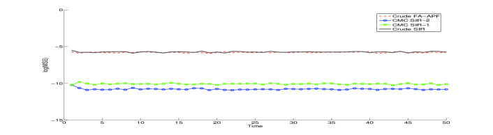
Figure 1: MSE - Gaussian model, $R=1$, $Q=10$, $N=1000$ - $f(x_{n})=x_{n}$. Estimator CMC-SIR-2 which propagates the samples with an FA algorithm outperforms CMC-SIR-1 which uses a SIR algorithm. Both CMC estimators outperform the crude ones.

2.4.2 ARCH Model

We next consider the ARCH model recalled in section 2.2.1 We set $R_{n}^{v}=3$, $\beta_{0}=1$ and $\beta_{1}=0.1$. We want to estimate $x_{n}$ (so $f(x_{n})=x_{n}$), and the variance of the process noise (so $f(x_{n})=\beta_{0}+\beta_{1}x_{n}^{2})$. Since $p(x_{n}|x_{n-1},y_{n})$ is Gaussian (see (25)), it is possible to calculate both moments. We compare $\widehat{\Theta}_{n}^{\rm FA}(1000)$ and $\widetilde{\Theta}_{n}^{{\rm SIR},2}(1000)$, both computed with $N=1000$ particles, and $\widetilde{\Theta}_{n}^{{\rm SIR},2}(100)$. MSEs are displayed on Fig. 2 for the estimate of $x_{n}$ and Fig. 3 for the variance of the process noise. As we see $\widetilde{\Theta}_{n}^{{\rm SIR},2}(1000)$, and even $\widetilde{\Theta}_{n}^{{\rm SIR},2}(100)$, both outperform $\widehat{\Theta}_{n}^{\rm FA}(1000)$. However the gap between the three algorithms is function dependent and so the previous considerations are model and function dependent.

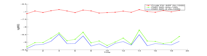
Figure 2: MSE - ARCH Model - $\beta_{0}=1$, $\beta_{1}=0.1$ and $R_{n}^{v}=3$ - $f(x_{n})=x_{n}$. The CMC estimator with $N=100$ particles outperforms the crude one with $N=1000$ particles and is close to the CMC one with $N=1000$ particles.

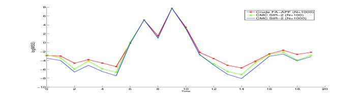
Figure 3: MSE - ARCH Model - $\beta_{0}=1$, $\beta_{1}=0.1$ and $R_{n}^{v}=3$ - $f(x_{n})=\beta_{0}+\beta_{1}x_{n-1}^{2}$. The gap between the three estimators depends on function $f(.)$ and has decreased compared to the previous simulation.

2.4.3 Stochastic Volatility Model

Let us consider the following model:

$$X_{n+1}= \Phi X_{n}+U_{n}$$ (32)

$$Y_{n}= \beta{\rm exp}(X_{n}/2)\times V_{n}$$ (33)

in which $U_{n}\sim\mathcal{N}(0,\sigma^{2})$ and $V_{n}\sim\mathcal{N}(0,1)$. In this model $\widetilde{\Theta}_{n}$ is not computable, whatever function $f$, because $p(y_{n}|x_{n-1})$ is not computable. We propose to compare two approximations of the Bayesian CMC estimator with a SIR based crude estimator. Our first approximation $\overline{\Theta}_{n}^{{\rm SIR},1}$ only relies on the approximation of $\int f(x_{n})p(x_{n}|x_{n-1},y_{n}){\rm d}x_{n}$ (second item in §2.2.2) while the second one $\overline{\Theta}_{n}^{{\rm SIR},2}$ relies in addition on that of $p(y_{n}|x_{n-1})$ (first item in §2.2.2). In this model, an approximation of $p(y_{n}|x_{n-1})$ is obtained by a first order Taylor series expansion of function ${\rm log}(g_{n}(y_{n}|x_{n}))$ in $\Phi x_{n-1}$. If the deduced approximation of $g_{n}(y_{n}|x_{n})$ is noted $\widehat{g}_{n}(y_{n}|x_{n})$ then $\widehat{p}(y_{n}|x_{n-1})=\int f_{n|n-1}(x_{n}|x_{n-1})\widehat{g}_{n}(y_{n}|x_{n}){\rm d}x_{n}$ where $f_{n|n-1}(x_{n}|x_{n-1})=\mathcal{N}(x_{n};\Phi x_{n-1};\sigma^{2})$, is now computable. If $\sigma$ is small, $f_{n|n-1}(x_{n}|x_{n-1})$ is approximately non-null for values close to $\Phi{\mathbf{x}}_{n-1}$, and for such values $\widehat{g}_{n}(y_{n}|x_{n})$ is a good approximation of $g_{n}(y_{n}|x_{n})$. So one should get a good approximation $\widehat{p}(y_{n}|x_{n-1})$ when $\sigma$ is small. Finally, a deduced approximation of $p(x_{n}|x_{n-1},y_{n})$ is given by a Gaussian pdf, see auxiliary .

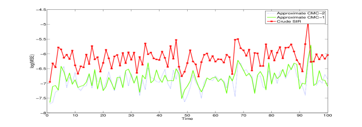
Figure 4: MSE - Stochastic Volatility Model - $\Phi=0.8$, $\beta=0.6$, $\sigma=0.18$, $N=1000$. Both approximate CMC estimators outperform the crude one.

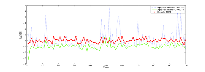
Figure 5: MSE - Stochastic Volatility Model - $\Phi=0.8$, $\beta=0.6$, $\sigma=0.4$, $N=1000$. Only the approximate estimator CMC-1 outperforms the crude estimator. This is because the approximation of $p({\mathbf{y}}_{n}|{\mathbf{x}}_{n-1})$ used by the approximate estimator CMC-2 is not reliable with these parameters.

We estimate the standard deviation of the observation noise at time $n$ so $f(x_{n})=\beta{\rm exp}(x_{n}/2)$. We first take $\Phi=0.8$, $\beta=0.6$, $\sigma=0.18$. Results are displayed in Fig. 4. We observe that both approximations of the Bayesian CMC estimator outperform the crude SIR-based one, and that the second approximation, which does not use ${\mathbf{x}}_{n}^{1:N}$, is preferable. However, in Fig. 5 we take $\sigma=0.40$. Remember that increasing $\sigma$ has consequences on the approximation of $p(y_{n}|x_{n-1})$; as expected, $\overline{\Theta}_{n}^{{\rm SIR},2}$, which relies on this approximation, is outperformed by the two other estimators. It is particularly interesting to notice that the first approximation $\overline{\Theta}_{n}^{{\rm SIR},1}$ is not affected and still outperforms the SIR based estimator. This confirms that Bayesian CMC estimators can still be of practical interest in models which are not semi-linear.

3 Bayesian CMC algorithms for JMSS models

As in §2 we still consider the estimation of $\Theta_{n}=\int\phi({\mathbf{x}}_{n})p({\mathbf{x}}_{n}|{\mathbf{y}}_{0:n}){\rm d}{\mathbf{x}}_{n}$ (the reason why we replaced $f$ by $\phi$ will become clear a few lines below), but now in a so-called JMSS:

$$p({\bf r}_{0:n},{\bf x}_{0:n},{\bf y}_{0:n})\!=\!p({r}_{0})\!\prod_{i=1}^{n}\!p({r}_{i}|{r}_{i-1})p({\bf x}_{0})\!\prod_{i=1}^{n}\!f_{i|i-1}({\bf x}_{i}|{\bf x}_{i-1},r_{i})\!\prod_{i=0}^{n}\!g_{i}({\bf y}_{i}|{\bf x}_{i},r_{i}).$$ (34)

Model (34) can be thought of as an HMC model, in which $f_{i|i-1}$ and $g_{i}$ depend on the realization of a discrete Markov Chain $\{R_{n}\}_{n\geq 0}$ where each $R_{n}$ takes its values in $\{1,\cdots,K\}$. So now both $X_{n}$ and $R_{n}$ are hidden, and $\Theta_{n}$ can be rewritten as

$$\Theta_{n}=\sum_{{\bf r}_{0:n}}\int\phi({\bf x}_{n})p({\bf x}_{n},{\bf r}_{0:n}|{\bf y}_{0:n}){\rm d}{\bf x}_{n}.$$ (35)

Note that $\phi(.)$ can also depend on $r_{n}$. As is well known tugnait shalom-li-kirubarajan doucet-jump-Mkv , in a JMSS exact Bayesian filtering is either impossible (in the general case) or an NP-hard problem (in the linear and Gaussian case), so one has to use suboptimal techniques. Among them, SMC methods can be divided into two classes:

• In the first class musso-oudjane-legland ginnity Cappeetal $\Theta_{n}$ is computed by injecting an SMC approximation of $p({\bf x}_{0:n},{\bf r}_{0:n}|{\bf y}_{0:n})$ into (35);

• In the second class of SMC methods we start from

  $$\Theta_{n}=\sum_{{\bf r}_{0:n}}\underbrace{p({\bf r}_{0:n}|{\bf y}_{0:n})}_{\rm PF}\int\phi({\bf x}_{n})\underbrace{p({\bf x}_{n}|{\bf r}_{0:n},{\bf y}_{0:n})}_{\rm KF}{\rm d}{\bf x}_{n},$$ (36)

  and propagate an SMC approximation $\sum_{i=1}^{N}w_{n}^{i}\delta_{{\bf r}_{0:n}^{i}}$ of $p({\bf r}_{0:n}|{\bf y}_{0:n})$ only; then $\widehat{\Theta}_{n}$ is computed as

  $$\widehat{\Theta}_{n}=\sum_{i=1}^{N}w_{n}^{i}\int\phi({\bf x}_{n})\underbrace{p({\bf x}_{n}|{\bf r}_{0:n}^{i},{\bf y}_{0:n})}_{\rm KF}{\rm d}{\bf x}_{n},$$ (37)

  in which $p({\bf x}_{n}|{\bf r}_{0:n}^{i},{\bf y}_{0:n})$ is computed exactly via KF if model (34), conditionally on ${\bf r}_{0:n}$, is linear and Gaussian, i.e. if $f_{i+1|i}({\bf x}_{i+1}|{\bf x}_{i},r_{i+1})$ and $g_{i}({\bf y}_{i}|{\bf x}_{i},r_{i})$ are Gaussian with means linear in ${\bf x}_{i}$ doucet-jump-Mkv .

3.1 Bayesian CMC algorithms for linear and Gaussian JMSS models

3.1.1 Deriving the Bayesian CMC algorithm

In this section we begin with the second class of algorithms. Let us first see that (36) coincides with (6) (in which the integral is replaced by a sum, since $R_{n}$ is discrete), up to the identification: $X_{1}={\bf R}_{0:n-1}$, $X_{2}=R_{n}$, $f(x_{1},x_{2})=\int\phi({\bf x}_{n})p({\bf x}_{n}|{\bf r}_{0:n-1},r_{n},{\bf y}_{0:n}){\rm d}{\bf x}_{n}$, and $p(x_{1},x_{2})$ is the joint pdf

$$p({\bf r}_{0:n}|{\bf y}_{0:n})=\underbrace{p({\bf r}_{0:n-1}|{\bf y}_{0:n})}_{p(x_{1})}\underbrace{p(r_{n}|{\bf r}_{0:n-1},{\bf y}_{0:n})}_{p(x_{2}|x_{1})}.$$ (38)

We need to compute both factors (we cannot simply apply the results of §2.1, because in (34) the marginal chain $(R_{n},{\bf Y}_{n})$ is not an HMC, as was $({\bf X}_{n},{\bf Y}_{n})$ in (13)). We first need an approximation of $p(x_{1})$, i.e. of

$$p({\bf r}_{0:n-1}|{\bf y}_{0:n})=\frac{p({\bf y}_{n}|{\bf r}_{0:n-1},{\bf y}_{0:n-1})p({\bf r}_{0:n-1}|{\bf y}_{0:n-1})}{\sum_{{\bf r}_{0:n-1}}p({\bf y}_{n}|{\bf r}_{0:n-1},{\bf y}_{0:n-1})p({\bf r}_{0:n-1}|{\bf y}_{0:n-1})}.$$ (39)

However the SMC algorithm propagates approximations of $p({\bf r}_{0:n}|{\bf y}_{0:n})$. So let $\widehat{p}({\bf r}_{0:n-1}|{\bf y}_{0:n-1})=$ $\sum_{i=1}^{N}w_{n-1}^{i}\delta_{{\bf r}_{0:n-1}^{i}}$; applying again Rubin’s SIR mechanism, $\widehat{p}({\bf r}_{0:n-1}|{\mathbf{y}}_{0:n})=\sum_{i=1}^{N}\widetilde{w}_{n-1}^{i}\delta_{{\bf r}_{0:n-1}^{i}}$, where

$$\widetilde{w}_{n-1}^{i}\propto{w}_{n-1}^{i}p({\mathbf{y}}_{n}|{\mathbf{y}}_{0:n-1},{\bf r}_{0:n-1}^{i}),\;\;\sum_{i=1}^{N}\widetilde{w}_{n-1}^{i}=1,$$ (40)

is an MC approximation of $p({\bf r}_{0:n-1}|{\mathbf{y}}_{0:n})$. Next from (34), the second factor $p(x_{2}|x_{1})$ of (38) can be rewritten as (here ${\cal N}$ stands for numerator):

$$p(r_{n}|{\bf r}_{0:n-1}^{i},{\mathbf{y}}_{0:n}) = \frac{p({\mathbf{y}}_{n}|{\mathbf{y}}_{0:n-1},{\bf r}_{0:n-1}^{i},r_{n})p(r_{n}|r_{n-1}^{i})}{p({\mathbf{y}}_{n}|{\mathbf{y}}_{0:n-1},{\mathbf{r}}_{0:n-1}^{i})=\sum_{r_{n}}{\cal N}}.$$ (41)

Note that as in section 2, $p(r_{n}|{\bf r}_{0:n-1}^{i},{\mathbf{y}}_{0:n})$ is the optimal conditional IS distribution, i.e. that which minimizes the conditional variance of the weights, given ${\bf r}_{0:n-1}^{i}$ and ${\mathbf{y}}_{0:n}$. Finally, setting $f({\bf r}_{0:n-1}^{i},r_{n})=$ ${\rm E}(\phi({\mathbf{x}}_{n})|{\mathbf{y}}_{0:n},{\bf r}_{0:n-1}^{i},r_{n})$, the Bayesian CMC and crude estimators respectively read

$$\widetilde{\Theta}_{n}({\bf r}_{0:n-1}^{1:N}) = \sum_{i=1}^{N}\widetilde{w}_{n-1}^{i}({\bf r}_{0:n-1}^{1:N})\sum_{r_{n}}f({\bf r}_{0:n-1}^{i},r_{n})p(r_{n}|{\bf r}_{0:n-1}^{i},{\bf y}_{0:n}),$$ (42)

$$\widehat{\Theta}_{n}({\bf r}_{0:n-1}^{1:N},{\bf r}_{n}^{1:N}) = \sum_{i=1}^{N}\widetilde{w}_{n-1}^{i}({\bf r}_{0:n-1}^{1:N})f({\bf r}_{0:n-1}^{i},r_{n}^{i}),$$ (43)

in which $r_{n}^{i}\sim$ $p(r_{n}|{\bf r}_{0:n-1}^{i},{\bf y}_{0:n})$.

3.1.2 Computing $\widetilde{\Theta}_{n}$ in practice: linear and Gaussian JMSS

Implementing $\widetilde{\Theta}_{n}$ requires that (40) and (41) are computable, and that in (42) the conditional expectation $f({\bf r}_{0:n-1}^{i},r_{n})$ is computable too. We thus need to compute $p({\mathbf{y}}_{n}|{\mathbf{y}}_{0:n-1},{\bf r}_{0:n-1}^{i},r_{n})$, which is not possible in general JMSS models. So let us now assume that the JMSS (34) is moreover linear and (conditionally) Gaussian:

$$R_{n}\text{ is a discrete Markov Chain},$$ (44)

$${\bf X}_{n}={\bf F}_{n}(R_{n}){\bf X}_{n-1}+{\bf G}_{n}(R_{n}){\bf U}_{n},$$ (45)

$${\bf Y}_{n}={\bf H}_{n}(R_{n}){\bf X}_{n}+{\bf L}_{n}(R_{n}){\bf V}_{n},$$ (46)

where ${\bf X}_{0}$, ${\bf U}_{1},\cdots,{\bf U}_{n}$ and ${\bf V}_{0},\cdots,{\bf V}_{n}$ are independent and independent of $R_{0},\cdots,R_{n}$. We set ${\bf X}_{0}\sim\mathcal{N}({\bf m}_{0},{\bf P}_{0})$, ${\bf U}_{n}\sim\mathcal{N}({\bf 0},{\bf Q}_{n})$ and ${\bf V}_{n}\sim\mathcal{N}({\bf 0},{\bf R}^{v}_{n})$. Then let $p({\bf x}_{n-1}|{\bf r}_{0:n-1}^{i},{\bf y}_{0:n-1})={\cal N}({\mathbf{x}}_{n-1};{\bf m}_{n-1|n-1}^{i};{\bf P}_{n-1|n-1}^{i}).$ Then $p({\bf y}_{n}|$ ${\bf y}_{0:n-1},{\bf r}_{0:n-1}^{i},r_{n})$ is given by the predicted observation mean and covariance of the KF, i.e.

$$p({\bf y}_{n}|{\bf y}_{0:n-1},{\bf r}_{0:n-1}^{i},r_{n})=\mathcal{N}({\bf y}_{n};\widetilde{\bf y}_{n}^{i}(r_{n});{\bf S}_{n}^{i}(r_{n})),$$ (47)

where

$$\widetilde{\bf y}_{n}^{i}(r_{n}) = {\bf y}_{n}-{\bf H}_{n}(r_{n}){\bf F}_{n}(r_{n}){\bf m}_{n-1|n-1}^{i}\text{,}$$ (48)

$${\bf S}_{n}^{i}(r_{n}) = {\bf H}_{n}(r_{n}){\bf P}_{n|n-1}^{i}(r_{n}){\bf H}_{n}(r_{n})^{T}+{\bf L}_{n}(r_{n}){\bf R}_{n}^{v}{\bf L}_{n}(r_{n})^{T}$$ (49)

$${\bf P}_{n|n-1}^{i}(r_{n}) = {\bf F}_{n}(r_{n}){\bf P}_{n-1|n-1}^{i}{\bf F}_{n}^{T}(r_{n})+{\bf G}_{n}(r_{n}){\bf Q}_{n}{\bf G}_{n}(r_{n})^{T}.$$ (50)

In summary, (47)-(50) enable to compute (40) and (41), and finally (42).

Remark 2

Estimator $\widetilde{\Theta}_{n}$ in (42) is the Bayesian CMC counterpart of $\widehat{\Theta}_{n}$ in (43), which itself coincides with the so-called RB SMC estimator (37) for JMSS doucet-jump-Mkv . Indeed, $\widehat{\Theta}_{n}$ corresponds to $\widehat{\Theta}^{\rm RB}$ in (5) where ${\mathbf{x}}_{1}={\mathbf{r}}_{0:n}$, ${\mathbf{x}}_{2}={\mathbf{x}}_{0:n}$, $f({\mathbf{x}}_{1},{\mathbf{x}}_{2})=\phi({\mathbf{x}}_{n})$ and $q_{1}(r_{n}|{\mathbf{r}}_{0:n-1})=p(r_{n}|{\bf r}_{0:n-1},{\bf y}_{0:n})$. So (42) can be seen as a further RB step of an already RB SMC estimator; the RB step leading to (37) was a spatial one, since PF was performed on variables ${\bf r}_{0:n}$, rather than on the extended state $({\bf x}_{0:n},{\bf r}_{0:n})$; here this second RB step is temporal, since in (42) PF acts on ${\bf r}_{0:n-1}$, rather than on ${\bf r}_{0:n}$. So here is an example where we can jointly use the classical RB-PF and our CMC Bayesian technique; but we will see in the next section that a CMC Bayesian estimator can also be derived in JMSS models in which classical RB-PF is not available.

Remark 3

One should observe that if $\widehat{\Theta}_{n}$ can be computed, $\widetilde{\Theta}_{n}$ can be computed as well; so the variance reduction can be achieved under the same assumptions (linear and Gaussian JMSS) as those needed for the RB SMC estimator doucet-jump-Mkv . On the other hand this new variance reduction involves an extra computational effort, which however is not prohibitive (at least if $K$ is small), as we see from (42) and (43). First, weights $\widetilde{w}_{n-1}^{i}$ in (40) have to be computed by both algorithms. Next for each $i$, $1\leq i\leq N$, both algorithms compute $\{p(r_{n}|{\bf r}_{0:n-1}^{i},{\bf y}_{0:n})\}_{r_{n}=1}^{K}$. The difference is that in the CMC algorithm we compute directly means $\sum_{r_{n}}f({\bf r}_{0:n-1}^{i},r_{n})p(r_{n}|{\bf r}_{0:n-1}^{i},{\bf y}_{0:n})$, which requires running $K$ KF updating steps per trajectory ${\bf r}_{0:n-1}^{i}$ while the crude estimator first extends randomly each trajectory before computing conditional expectations.

Remark 4

Finally our Bayesian CMC estimator $\widetilde{\Theta}_{n}$ stems from the RB PF which, itself, assumes that the JMSS model is conditionally linear with additive Gaussian noise. If this is not the case, but the non-linearities are not too severe, one can approximate ${\rm E}(\phi({\mathbf{x}}_{n})|{\mathbf{y}}_{0:n},{\bf r}_{0:n})$ by EKF or UKF, and next compute $\widetilde{\Theta}_{n}$ from such an approximation, by using an approximation of $p({\mathbf{y}}_{n}|{\mathbf{y}}_{0:n-1},{\bf r}_{0:n})$, also given by EKF or UKF.

3.2 Bayesian CMC algorithms for non linear JMSS models

In this section we derive Bayesian CMC estimators in non linear JMSS models, in the case where, by contrast with Remark 4 above, it is not possible to approximate ${\rm E}(\phi({\mathbf{x}}_{n})|{\mathbf{y}}_{0:n},{\bf r}_{0:n})$. In that case we need to turn back to the first class of SMC methods for JMSS (see the beginning of section 3), which consists in propagating an SMC approximation of $p({\mathbf{x}}_{0:n},{\mathbf{r}}_{0:n}|{\mathbf{y}}_{0:n})$ doucet-jump-Mkv Andrieux-JM .

3.2.1 Deriving Bayesian CMC estimators

Let us first rewrite $\Theta_{n}$ as

$$\Theta_{n} =\sum_{{\mathbf{r}}_{0:n-1},r_{n}}\int\phi({\mathbf{x}}_{n})p({\mathbf{x}}_{0:n-1},{\mathbf{r}}_{0:n-1},{\mathbf{x}}_{n},r_{n}|{\mathbf{y}}_{0:n}){\rm d}{\mathbf{x}}_{0:n-1}{\rm d}{\mathbf{x}}_{n}\text{.}$$ (51)

Let now $\sum_{i=1}^{N}w_{n-1}^{i}({\bf x}_{0:n-1}^{1:N},{\bf r}_{0:n-1}^{1:N})\delta_{{\mathbf{x}}_{0:n-1}^{i},{\mathbf{r}}_{0:n-1}^{i}}$ be an MC approximation of $p({\mathbf{x}}_{0:n-1},$ ${\mathbf{r}}_{0:n-1}|{\mathbf{y}}_{0:n-1})$. Then $\widehat{p}({\mathbf{x}}_{0:n-1},{\mathbf{r}}_{0:n-1}|{\mathbf{y}}_{0:n})=\sum_{i=1}^{N}\widetilde{w}_{n-1}^{i}\delta_{{\mathbf{x}}_{0:n-1}^{i},{\mathbf{r}}_{0:n-1}^{i}}$, in which

$$\widetilde{w}_{n-1}^{i} \propto w_{n-1}^{i}p({\mathbf{y}}_{n}|{\mathbf{x}}_{n-1}^{i},r_{n-1}^{i}),\sum_{i=1}^{N}\widetilde{w}_{n-1}^{i}=1$$ (52)

is an MC approximation of $p({\mathbf{x}}_{0:n-1},{\mathbf{r}}_{0:n-1}|{\mathbf{y}}_{0:n})$. Let also

$$({\mathbf{x}}_{n}^{i},r_{n}^{i})\sim p({\mathbf{x}}_{n},r_{n}|{\mathbf{x}}_{n-1}^{i},r_{n-1}^{i},{\mathbf{y}}_{n})\text{.}$$ (53)

Then the associated crude MC estimator is given by doucet-jump-Mkv Andrieux-JM :

$$\widehat{\Theta}_{n}({\bf x}_{0:n}^{1:N},{\bf r}_{0:n}^{1:N}) = \sum_{i=1}^{N}\widetilde{w}_{n-1}^{i}({\bf x}_{0:n-1}^{1:N},{\bf r}_{0:n-1}^{1:N})\phi({\mathbf{x}}_{n}^{i}),$$ (54)

We now propose two Bayesian CMC estimators of $\Theta_{n}$, associated to two different partitions of $({\bf X}_{0:n},{\bf R}_{0:n})$. Setting $X_{1}=({\bf X}_{0:n-1},{\bf R}_{0:n})$ and $X_{2}={\bf X}_{n}$ leads to $\widetilde{\Theta}_{n}^{{\bf X}_{n}}$; setting $X_{1}=({\bf X}_{0:n-1},{\bf R}_{0:n-1})$, $X_{2}=({\bf X}_{n},R_{n})$ and $f({\mathbf{x}}_{n-1}^{i},{\mathbf{y}}_{n},$ ${\mathbf{r}}_{n})=\int\phi({\mathbf{x}}_{n})p({\mathbf{x}}_{n}|{\mathbf{x}}_{n-1}^{i},r_{n},{\mathbf{y}}_{n}){\rm d}{\mathbf{x}}_{n}$ leads to $\widetilde{\Theta}_{n}^{({\bf X}_{n},R_{n})}$, with

$$\widetilde{\Theta}^{{\bf X}_{n}}_{n}\!({\bf x}_{0:n-1}^{1:N},{\bf r}_{0:n}^{1:N}) \!\!=\!\! \sum_{i=1}^{N}\widetilde{w}_{n-1}^{i}f({\mathbf{x}}_{n-1}^{i},{\mathbf{y}}_{n},{\mathbf{r}}_{n}^{i}),$$ (55)

$$\widetilde{\Theta}_{n}^{({\bf X}_{n},R_{n})}({\bf x}_{0:n-1}^{1:N},{\bf r}_{0:n-1}^{1:N}) \!\!=\!\! \sum_{i=1}^{N}\!\widetilde{w}_{n-1}^{i}\!\!\sum_{r_{n}}\!\!\int\!\!\phi({\mathbf{x}}_{n})p({\mathbf{x}}_{n},r_{n}|{\mathbf{x}}_{n-1}^{i},r_{n-1}^{i},{\mathbf{y}}_{n}){\rm d}{\mathbf{x}}_{n}$$

$$\!\!=\!\! \sum_{i=1}^{N}\widetilde{w}_{n-1}^{i}\!\!\sum_{r_{n}}p(r_{n}|{\mathbf{x}}_{n-1}^{i},r_{n-1}^{i},{\mathbf{y}}_{n})f({\mathbf{x}}_{n-1}^{i},{\mathbf{y}}_{n},{\mathbf{r}}_{n}),$$

in which $\widetilde{w}_{n-1}^{i}({\bf x}_{0:n-1}^{1:N},{\bf r}_{0:n-1}^{1:N})$ is given by (52), and in (55) $r_{n}^{i}\sim p(r_{n}|{\mathbf{x}}_{n-1}^{i},$ $r_{n-1}^{i},{\mathbf{y}}_{n})$ (a marginal of (53)). Of course, $\widetilde{\Theta}^{{\bf X}_{n}}_{n}={\rm E}(\widehat{\Theta}_{n}|{\mathbf{x}}_{0:n-1}^{1:N},r_{0:n}^{1:N},{\mathbf{y}}_{0:n})$ and $\widetilde{\Theta}_{n}^{({\bf X}_{n},R_{n})}={\rm E}(\widetilde{\Theta}^{{\bf X}_{n}}_{n}|{\mathbf{x}}_{0:n-1}^{1:N},r_{0:n-1}^{1:N},{\mathbf{y}}_{0:n})$, so ${\rm var}(\widetilde{\Theta}_{n}^{({\bf X}_{n},R_{n})})\leq{\rm var}(\widetilde{\Theta}_{n}^{{\bf X}_{n}})\leq{\rm var}(\widehat{\Theta}_{n})$.

3.2.2 Computing $\widetilde{\Theta}_{n}^{{\bf X}_{n}}$ and $\widetilde{\Theta}_{n}^{({\bf X}_{n},R_{n})}$ in practice

Let us now discuss when (55) and (3.2.1) can be computed. In model (34), $p({\mathbf{y}}_{n}|{\mathbf{x}}_{n-1}^{i},r_{n-1}^{i})=\sum_{r_{n}}p(r_{n}|r_{n-1}^{i})p({\mathbf{y}}_{n}|{\mathbf{x}}_{n-1}^{i},r_{n})$ and $p({\mathbf{y}}_{n}|{\mathbf{x}}_{n-1}^{i},r_{n-1}^{i})p({\mathbf{x}}_{n},$ $r_{n}|{\mathbf{x}}_{n-1}^{i},r_{n-1}^{i},{\mathbf{y}}_{n})=p(r_{n}|r_{n-1}^{i})p({\mathbf{y}}_{n}|{\mathbf{x}}_{n-1}^{i},r_{n})p({\mathbf{x}}_{n}|{\mathbf{x}}_{n-1}^{i},r_{n},{\mathbf{y}}_{n})$. So let

$$\overline{w}_{n-1}^{i}(r_{n}) = \frac{w_{n-1}^{i}p(r_{n}|r_{n-1}^{i})p({\mathbf{y}}_{n}|{\mathbf{x}}_{n-1}^{i},r_{n})}{\sum_{r_{n}}\sum_{i=1}^{N}w_{n-1}^{i}p(r_{n}|r_{n-1}^{i})p({\mathbf{y}}_{n}|{\mathbf{x}}_{n-1}^{i},r_{n}^{i})}$$ (57)

(note that $\sum_{r_{n}}\overline{w}_{n-1}^{i}(r_{n})=$ $\widetilde{w}_{n-1}^{i}$). Then $\widetilde{\Theta}_{n}^{{\bf X}_{n}}$ and $\widetilde{\Theta}_{n}^{({\bf X}_{n},R_{n})}$ can be rewritten as

$$\widetilde{\Theta}_{n}^{{\bf X}_{n}} = \sum_{i=1}^{N}\left[\sum_{r_{n}}\overline{w}_{n-1}^{i}(r_{n})\right]\int\phi({\mathbf{x}}_{n})p({\mathbf{x}}_{n}|{\mathbf{x}}_{n-1}^{i},{\mathbf{y}}_{n},r_{n}^{i}){\rm d}{\mathbf{x}}_{n},$$ (58)

$$\widetilde{\Theta}_{n}^{({\bf X}_{n},R_{n})} = \sum_{i=1}^{N}\left[\sum_{r_{n}}\overline{w}_{n-1}^{i}(r_{n})\int\phi({\mathbf{x}}_{n})p({\mathbf{x}}_{n}|{\mathbf{x}}_{n-1}^{i},{\mathbf{y}}_{n},r_{n}){\rm d}{\mathbf{x}}_{n}\right].$$ (59)

So (59) is computable as soon as (58) is computable. On the other hand, $\widetilde{\Theta}_{n}^{{\bf X}_{n}}$ is a generalization of (19): $p({\mathbf{x}}_{n}|{\mathbf{x}}_{n-1},{\mathbf{y}}_{n},r_{n})$ and $p({\mathbf{y}}_{n}|{\mathbf{x}}_{n-1},r_{n})$ play the same role as $p({\mathbf{x}}_{n}|{\mathbf{x}}_{n-1},{\mathbf{y}}_{n})$ and $p({\mathbf{y}}_{n}|{\mathbf{x}}_{n-1})$ in §2.1 except that we have now introduced a dependency in $r_{n}$. This means that $\widetilde{\Theta}_{n}^{{\bf X}_{n}}$ and $\widetilde{\Theta}_{n}^{({\bf X}_{n},R_{n})}$ are computable as soon as the Bayesian CMC estimator (19) of §2.1 is computable in the underlying HMC model (i.e., the HMC model to which the JMSS reduces when the jumps are known), see section 2.2.1. For example, semi-linear stochastic models (including the ARCH ones) with Markov jumps are a class of models in which (58) and (59) are computable.

Finally the only difference between (58) and (59) comes from the computational cost that we discuss now. For a given $i$, in (59) the computation of $\int\phi({\mathbf{x}}_{n})p({\mathbf{x}}_{n}|{\mathbf{x}}_{n-1}^{i},r_{n},{\mathbf{y}}_{n}){\rm d}{\mathbf{x}}_{n}$ has to be done for all $r_{n}$, while in (58) it has only to be done for the $r_{n}^{i}$ which has been sampled. So as expected, $\widetilde{\Theta}_{n}^{({\bf X}_{n},R_{n})}$ is preferable to $\widetilde{\Theta}_{n}^{{\bf X}_{n}}$ but requires an extra computational cost. On the other hand, comparing the computational cost of $\widetilde{\Theta}_{n}^{{\bf X}_{n}}$ and $\widehat{\Theta}_{n}$ is the same issue as comparing that of the Bayesian CMC estimator (19) to that of the crude MC one (18) in Section 2.2, and is thus problem dependent. However, one should observe that in the particular case described at the end of section 2.2.1, i.e. when sampling according to $p({\mathbf{x}}_{n}|{\mathbf{x}}_{n-1},r_{n},{\mathbf{y}}_{n})$ requires the computation of $\int\phi({\mathbf{x}}_{n})p({\mathbf{x}}_{n}|{\mathbf{x}}_{n-1},r_{n},{\mathbf{y}}_{n}){\rm d}{\mathbf{x}}_{n}$, then the computation of $\widetilde{\Theta}_{n}^{{\bf X}_{n}}$ does not involve an extra computational cost as compared to that of $\widehat{\Theta}_{n}$.

3.2.3 Approximate computation

Let us finally discuss on approximate computation of $\widetilde{\Theta}_{n}$ when $p({\mathbf{y}}_{n}|{\mathbf{x}}_{n-1},r_{n})$ and $p({\mathbf{x}}_{n}|{\mathbf{x}}_{n-1},{\mathbf{y}}_{n},r_{n})$ in (59) are not available. First notice that (59) can be computed with the same numerical approximations as those which were used in the computation of (19) (see section 2.2.2 above), except that they have to be done for all possible values of $r_{n}$. However, $r_{n}$ is discrete and as we now see, one can derive other approximation techniques:

• In (34) we have $p(r_{n},{\mathbf{x}}_{n},{\mathbf{y}}_{n}|{\mathbf{x}}_{n-1},r_{n-1})=p(r_{n}|r_{n-1})f_{n|n-1}({\mathbf{x}}_{n}|{\mathbf{x}}_{n-1},r_{n})$ $g_{n}({\mathbf{y}}_{n}|{\mathbf{x}}_{n},r_{n})$ so the numerator of (59) can be rewritten as

  $$\sum_{r_{n}}\int\phi({\mathbf{x}}_{n})\left[\sum_{i=1}^{N}p(r_{n}|r_{n-1}^{i})w_{n-1}^{i}f_{n|n-1}({\mathbf{x}}_{n}|{\mathbf{x}}_{n-1}^{i},r_{n})g_{n}({\mathbf{y}}_{n}|{\mathbf{x}}_{n},r_{n})\right]{\rm d}{\mathbf{x}}_{n}.$$

  If for a given $r_{n}$ the integral is not computable, one can approximate it with IS by sampling ${\mathbf{x}}_{n}^{r_{n},i}\sim q({\mathbf{x}}_{n}|{\mathbf{x}}_{n-1}^{i},r_{n})$ for all $i$, $1\leq i\leq N$ and for all $r_{n}$. An approximation of the numerator is then given by $\sum_{r_{n}}\sum_{i=1}^{N}\phi({\mathbf{x}}_{n}^{r_{n},i})$ $p(r_{n}|r_{n-1}^{i})w_{n-1}^{i}f_{n|n-1}({\mathbf{x}}_{n}^{r_{n},i}|{\mathbf{x}}_{n-1}^{i},r_{n})g_{n}({\mathbf{y}}_{n}|{\mathbf{x}}_{n}^{r_{n},i},r_{n})/q({\mathbf{x}}_{n}^{r_{n},i}|{\mathbf{x}}_{n-1}^{i},r_{n})$. So we do not use samples for the discrete part $r_{n}$. We apply the same approximation for the denominator which can be rewritten as $\sum_{r_{n}}\sum_{i=1}^{N}w_{n-1}^{i}$ $p(r_{n}|r_{n-1}^{i})\times\int f_{n|n-1}({\mathbf{x}}_{n}|r_{n},{\mathbf{x}}_{n-1}^{i})g_{n}({\mathbf{y}}_{n}|{\mathbf{x}}_{n},r_{n}){\rm d}{\mathbf{x}}_{n}$;

• When the optimal distribution $p({\mathbf{x}}_{n},r_{n}|{\mathbf{x}}_{n-1},r_{n-1},{\mathbf{y}}_{n})$ is not available, it has been proposed doucet-jump-Mkv to sample independently $({\mathbf{x}}_{n}^{i},r_{n}^{i})$ according to an importance distribution $q({\mathbf{x}}_{n},r_{n}|{\mathbf{x}}_{n-1}^{i},r_{n-1}^{i})=q(r_{n}|{\mathbf{x}}_{n-1}^{i},r_{n-1}^{i})q({\mathbf{x}}_{n}|{\mathbf{x}}_{n-1}^{i},$ $r_{n},r_{n-1}^{i})$, for all $i$, $1\leq i\leq N$, then to compute the estimator $\widehat{\Theta}^{\rm SIR}_{n}=\sum_{i=1}^{N}\frac{w_{n}^{i}}{\sum_{i=1}^{N}w_{n}^{i}}\phi({\mathbf{x}}_{n}^{i})$, $w_{n}^{i}=w_{n-1}^{i}\frac{p(r_{n}^{i}|r_{n-1}^{i})f_{n|n-1}({\mathbf{x}}_{n}^{i}|r_{n}^{i},{\mathbf{x}}_{n-1}^{i})g_{n}({\mathbf{y}}_{n}|{\mathbf{x}}_{n}^{i},r_{n}^{i})}{q({\mathbf{x}}_{n}^{i},r_{n}^{i}|{\mathbf{x}}_{n-1}^{i},r_{n-1}^{i})}$. Remember that the Bayesian CMC estimator $\widetilde{\Theta}_{n}$ is actually the expectation of the crude MC estimator $\widehat{\Theta}_{n}$ given some variables. One can wonder if it is not possible to compute ${\rm E}(\widehat{\Theta}_{n}^{\rm SIR}|\{r_{n-1}^{i},{\mathbf{x}}_{n-1}^{i},{\mathbf{x}}_{n}^{i}\}_{i=1}^{N},{\mathbf{y}}_{n})$, i.e. to compute the expectation of $\widehat{\Theta}^{\rm SIR}_{n}$ as a function of $r_{n}$. Since $\phi(.)$ does not depend on $r_{n}$, it is equivalent to compute the conditional expectation of the unnormalized weights $w_{n}^{i}$ and so to reduce their variance. Unfortunately this is not possible because of the normalization factor. However one can compute separately the conditional expectation of the numerator and that of the denominator. This is an easy task since $r_{n}$ takes its values in a discrete set, and $q(r_{n}|{\mathbf{x}}_{n},{\mathbf{x}}_{n-1},r_{n-1})\!\!=\!q(r_{n}|{\mathbf{x}}_{n-1},r_{n-1})q({\mathbf{x}}_{n}|{\mathbf{x}}_{n-1},r_{n},r_{n-1})\!/\!\sum_{r_{n}}\!q(r_{n}|{\mathbf{x}}_{n-1},$ $r_{n-1})q({\mathbf{x}}_{n}|{\mathbf{x}}_{n-1},r_{n},r_{n-1})$. This variance reduction of the unnormalized weights comes from a normalized IS implementation of (59) which is rewritten as

  $$\widetilde{\Theta}_{n}=$$

  $$\frac{\int\phi({\mathbf{x}}_{n})\sum_{i=1}^{N}\left[\sum_{r_{n}}p(r_{n}|r_{n-1}^{i})w_{n-1}^{i}f_{n|n-1}({\mathbf{x}}_{n}|{\mathbf{x}}_{n-1}^{i},r_{n})g_{n}({\mathbf{y}}_{n}|{\mathbf{x}}_{n},r_{n})\right]{\rm d}{\mathbf{x}}_{n}}{\int\sum_{i=1}^{N}\left[\sum_{r_{n}}p(r_{n}|r_{n-1}^{i})w_{n-1}^{i}f_{n|n-1}({\mathbf{x}}_{n}|{\mathbf{x}}_{n-1}^{i},r_{n})g_{n}({\mathbf{y}}_{n}|{\mathbf{x}}_{n},r_{n})\right]{\rm d}{\mathbf{x}}_{n}}\text{}$$ (60)

  with the importance distribution

  $$q({\mathbf{x}}_{n}|{\mathbf{x}}_{n-1},r_{n-1})=\sum_{r_{n}}q(r_{n}|{\mathbf{x}}_{n-1},r_{n-1})q({\mathbf{x}}_{n}|{\mathbf{x}}_{n-1},r_{n},r_{n-1})\text{.}$$

  Note that the computation of the new weights is not prohibitive as long as $K<<N$.

3.3 Simulations

We now test our approach in a linear and Gaussian JMSS model, described by equations (44)-(46) in which

$${\bf F}_{n}(r)=\begin{bmatrix}1&\frac{\sin(\omega_{r}T)}{\omega_{r}}&0&-\frac{1-\cos(\omega_{r}T)}{\omega_{r}}\\ 0&\cos(\omega_{r}T)&0&-\sin(\omega_{r}T)\\ 0&\frac{1-\cos(\omega_{r}T)}{\omega_{r}}&1&\frac{\sin(\omega_{r}T)}{\omega_{r}}\\ 0&\sin(\omega_{r}T)&0&\cos(\omega_{r}T)\end{bmatrix}\text{, }{\bf Q}_{n}=\sigma_{v}^{2}\begin{bmatrix}\frac{T^{3}}{3}&\frac{T^{2}}{2}&0&0\\ \frac{T^{2}}{2}&T&0&0\\ 0&0&\frac{T^{3}}{3}&\frac{T^{2}}{2}\\ 0&0&\frac{T^{2}}{2}&T\end{bmatrix}\text{, }$$

${\bf H}_{n}=\begin{bmatrix}1&0&0&0\\ 0&0&1&0\end{bmatrix}$, ${\bf R}_{n}=\begin{pmatrix}\sigma_{x}^{2}&0\\ 0&\sigma_{y}^{2}\end{pmatrix}\text{ and}$ ${\bf G}_{n}(r)={\bf I}$, $T=2s$, $\sigma_{v}=3m^{2}/sec^{3}$ and $\sigma_{x}=\sigma_{y}=10m$. We track a maneuvering target described by its position and velocity in the Cartesian coordinates, ${\mathbf{x}}_{n}=[p_{x},\dot{p}_{x},p_{y},\dot{p}_{y}]^{T}_{n}$. Mode $r_{n}$ represents the behavior of the target: straight, left turn and right turn. Remember from 3.1.2 that the computation of $\widetilde{\Theta}_{n}$ involves an extra computational cost compared to that of $\widehat{\Theta}_{n}$. So we compute the efficiency over $P=200$ simulations defined as lecuyer

$${\rm Eff}(n)=\frac{1}{{\rm MSE}(n){\rm E}(C(n))}\text{,}$$ (61)

where $C(n)$ is the CPU time to compute the estimator, and we discuss the performances of $\widehat{\Theta}_{n}$ and $\widetilde{\Theta}_{n}$ in function of the model parameters. Both estimators are computed with $N=1000$ particles.

We first set $\omega_{1}=0\text{ rad}.\text{s}^{-1}$, $\omega_{2}=3\pi/180\text{ rad}.\text{s}^{-1}$ and $\omega_{3}=-3\pi/180\text{ rad}.\text{s}^{-1}$. The Markovian transition probability is $p(r_{n}|r_{n-1})=0.4$ if $r_{n}=r_{n-1}$ and $p(r_{n}|r_{n-1})=0.3$ otherwise. In Figure 6, we display the (averaged) efficiency of both estimators over time. The efficiency of $\widetilde{\Theta}_{n}$ is greater than that of $\widehat{\Theta}_{n}$, so the Bayesian CMC estimator for linear JMSS is of practical interest. Note that the dependency of the model in $\{r_{n}\}$ is weak since $w_{r}$ is small and the Markovian transition probabilities are close. So distributions $\{p(r_{n}|{\mathbf{r}}_{0:n-1}^{i},{\mathbf{y}}_{0:n})\}_{i=1}^{N}$ tend to be uniform, and remember that $\widetilde{\Theta}_{n}$ computes directly the expectations according to these distributions while $\widehat{\Theta}_{n}$ uses samples ${\bf r}_{n}^{1:N}$ according to them. This is why the gap between both estimators gets larger when distributions $\{p(r_{n}|{\mathbf{r}}_{0:n-1}^{i},{\mathbf{y}}_{0:n})\}_{i=1}^{N}$ become almost uniform.

Next we increase the dependency of the model in $\{r_{n}\}$ by setting $\omega_{1}=0\text{ rad}.\text{s}^{-1}$, $\omega_{2}=8\pi/180\text{ rad}.\text{s}^{-1}$ and $\omega_{3}=-8\pi/180\text{ rad}.\text{s}^{-1}$. We also set $p(r_{k}|r_{k-1})=0.6$ if $r_{k}=r_{k-1}$ and $p(r_{k}|r_{k-1})=0.2$ otherwise. In Figure 7, we display the averaged efficiency of both estimators for this new set of parameters. Indeed, the gap between both estimators is reduced but $\widetilde{\Theta}_{n}$ still outperforms $\widehat{\Theta}_{n}$.

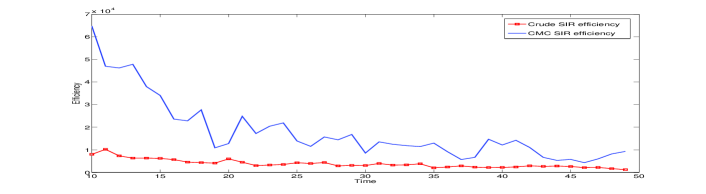
Figure 6: Efficiency - Linear JMSS Model - Close Markovian transition probabilities - $\phi({\mathbf{x}}_{n})={\mathbf{x}}_{n}$. Due to the weak dependency of the model in ${\mathbf{r}}_{n}$, it is dangerous to sample new particles (Crude SIR) before computing the estimator.

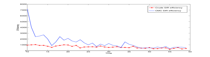
Figure 7: Efficiency - Linear JMSS Model - Dispersed Markovian transition probabilities - $\phi({\mathbf{x}}_{n})={\mathbf{x}}_{n}$. Contrary to the previous simulation, distributions $\{p(r_{n}|{\mathbf{r}}_{0:n-1}^{i},{\mathbf{y}}_{0:n})\}_{i=1}^{N}$ are dispersed so the gap between the crude SIR estimator and the CMC SIR one shrinks.

4 Bayesian CMC algorithms for Multi-Target filtering

In this final section we apply CMC to multi-target filtering. Some adaptations are necessary, because in the multi-target context we do not necessary deal with classical pdf. However, the discussion in section 1.3 still holds, as we shall see. Let us begin with a brief review of multi-object filtering.

4.1 A brief review of Random Finite Sets (RFS) based multi-target filtering

Multi-object filtering extends the previous problem in the sense that we now look for estimating an unknown number of targets from a set of observations which are either due to detected targets or are false alarms measurements. Classical solutions such as the Joint Probabilist Data association filter SHALOM_JPDAshort or the Multiple Hypothesis Tracker BLACKMAN include a matching mechanism between targets and observations. Alternate solutions are based on RFS, which are sets of random variables with random and time-varying cardinal (see e.g. MAHLER_LIVRE2007 ). The interest of RFS based techniques over classical solutions is that they no longer require such a matching mechanism. The RFS formulation was first used to derive the multi-object Bayesian filter, which generalizes the classical single object one MAHLER_ARTICLE2003 . This multi-object Bayesian filter involves the computation of set integrals of multi-object densities, i.e. of positive functions $f(X)$ of a given RFS $X$, and cannot be computed in practice (SMC approximations can however be of interest when the number of targets is small VO_SMC_PHD ). Later on, Mahler proposed to propagate a first order moment of the multi-object density, the so-called PHD or intensity MAHLER_ARTICLE2003 . Let $|X\cap S|$ be the number of objects in RFS $X$ which belong to region $S$; then the PHD $v({\mathbf{x}})$ is defined as the spatial density of the expected number of targets, i.e.

$$\int_{S\ \subset{\rm I\!R}^{p}}v({\mathbf{x}})\,\mathrm{\rm d}{\mathbf{x}}={\rm E}(|X\cap S|)\text{.}$$ (62)

Its interest in multi-object filtering is twofold; first, $\int v({\mathbf{x}}){\rm d}{\mathbf{x}}$ is an estimate of the number of targets; in addition, extracting the states consists in looking for regions where the PHD is high, and so local maxima of $v$ are required. Let now $v_{n}({\mathbf{x}})$ be the a posteriori PHD, i.e. the first order moment $v_{n}({\mathbf{x}})$ of the multi-object density at time $n$, given the set of past measurements $Z_{0:n}=\{Z_{1},\cdots,Z_{n}\}$, where $Z_{k}$ is the set of measurements available at time $k$. The PHD filter is a set of equations which enables to propagate $v_{n}$ and which has the advantage to make use of classical integrals only. If we assume that the cardinality distributions of the number of targets and of false alarm measurements are Poisson, and that each target evolves and generates observations independently of one another, then PHD $v_{n}$ is propagated as follows (we assume for simplicity that there is no spawning) MAHLER_ARTICLE2003 MAHLER_LIVRE2007 :

$$v_{n|n-1}({\mathbf{x}}_{n}) = \!\!\int\!\!p_{s,n}({\mathbf{x}}_{n-1})f_{n|n-1}({\mathbf{x}}_{n}|{\mathbf{x}}_{n-1})v_{n-1}({\mathbf{x}}_{n-1}){\rm d}{\mathbf{x}}_{n-1}+\gamma_{n}({\mathbf{x}}_{n})\text{,}$$ (63)

$$v_{n}({\mathbf{x}}_{n}) = \left[1-p_{d,n}({\mathbf{x}}_{n})\right]v_{n|n-1}({\mathbf{x}}_{n})$$ (64)

$$+ \sum_{{\mathbf{z}}\in Z_{n}}\frac{p_{d,n}({\mathbf{x}}_{n})g_{n}({\mathbf{z}}|{\mathbf{x}}_{n})v_{n|n-1}({\mathbf{x}}_{n})}{\kappa_{n}({\mathbf{z}})+\int p_{d,n}({\mathbf{x}}_{n})g_{n}({\mathbf{z}}|{\mathbf{x}}_{n})v_{n|n-1}({\mathbf{x}}_{n})\,{\rm d}{\mathbf{x}}_{n}}\text{,}$$

where $p_{s,n}(.)$ (resp. $p_{d,n}(.)$) is the probability of survival (resp. of detection) at time $n$ which can depend on state ${\mathbf{x}}_{n-1}$ (resp. on ${\mathbf{x}}_{n}$); and $\kappa_{n}(.)$ (resp. $\gamma_{n}(.)$) is the intensity of the false alarms measurements (resp. of the birth targets) at time $n$.

4.2 Deriving the Bayesian CMC PHD estimator

Let us now turn back to the derivation of a Bayesian CMC PHD estimator. First, the problem we address is to compute the moment $\Theta_{n}=\int f({\mathbf{x}}_{n})v_{n}({\mathbf{x}}_{n}){\rm d}{\mathbf{x}}_{n}$ (typically, we shall take either $f({\mathbf{x}}_{n})=1$ or $f({\mathbf{x}}_{n})={\bf 1}_{S}({\mathbf{x}}_{n})$, where $S$ is some region of interest). From now on we assume that $p_{d,n}$ does not depend on ${\mathbf{x}}_{n}$. Plugging (63) in (64), the PHD at time $n$ can be written as

$$v_{n}({\mathbf{x}}_{n})=\sum_{i=1}^{4}v_{n}^{i}({\mathbf{x}}_{n})\text{,}$$ (65)

where

$$v_{n}^{1}({\mathbf{x}}_{n}) =\left[1-p_{d,n}\right]\int p_{s,n}({\mathbf{x}}_{n-1})f_{n|n-1}({\mathbf{x}}_{n}|{\mathbf{x}}_{n-1})v_{n-1}({\mathbf{x}}_{n-1}){\rm d}{\mathbf{x}}_{n-1}\text{,}$$ (66)

$$v_{n}^{2}({\mathbf{x}}_{n}) =\left[1-p_{d,n}\right]\gamma_{n}({\mathbf{x}}_{n})\text{,}$$ (67)

$$v_{n}^{3}({\mathbf{x}}_{n})\!\! =\!\!\!\!\!\sum_{{\mathbf{z}}\in Z_{n}}\!\!\frac{\!p_{d,n}g_{n}({\mathbf{z}}|{\mathbf{x}}_{n})\!\!\int\!p_{s,n}({\mathbf{x}}_{n-1})\!f_{n|n-1}({\mathbf{x}}_{n}|{\mathbf{x}}_{n-1})v_{n-1}({\mathbf{x}}_{n-1}){\rm d}{\mathbf{x}}_{n-1}}{B_{n}({\mathbf{z}})}\text{,}$$ (68)

$$v_{n}^{4}({\mathbf{x}}_{n}) =\sum_{{\mathbf{z}}\in Z_{n}}\frac{p_{d,n}g_{n}({\mathbf{z}}|{\mathbf{x}}_{n})\gamma_{n}({\mathbf{x}}_{n})}{B_{n}({\mathbf{z}})}\text{,}$$ (69)

and where

$$B_{n}({\mathbf{z}}) =\kappa_{n}({\mathbf{z}})+B^{1}_{n}({\mathbf{z}})+B^{2}_{n}({\mathbf{z}})\text{,}$$ (70)

$$B^{1}_{n}({\mathbf{z}})\! =\!\int p_{d,n}g_{n}({\mathbf{z}}|{\mathbf{x}}_{n})\int p_{s,n}({\mathbf{x}}_{n-1})f_{n|n-1}({\mathbf{x}}_{n}|{\mathbf{x}}_{n-1})v_{n-1}({\mathbf{x}}_{n-1}){\rm d}{\mathbf{x}}_{n-1}{\rm d}{\mathbf{x}}_{n}$$

$$=p_{d,n}\int p_{s,n}({\mathbf{x}}_{n-1})p({\mathbf{z}}|{\mathbf{x}}_{n-1})v_{n-1}({\mathbf{x}}_{n-1}){\rm d}{\mathbf{x}}_{n-1}\text{,}$$ (71)

$$B^{2}_{n}({\mathbf{z}}) =\int p_{d,n}g_{n}({\mathbf{z}}|{\mathbf{x}}_{n})\gamma_{n}({\mathbf{x}}_{n}){\rm d}{\mathbf{x}}_{n}\text{.}$$ (72)

Term $v_{n}^{1}$ (resp. $v_{n}^{2}$) is due to non-detected persistent (resp. birth) targets, while $v_{n}^{3}$ (resp. $v_{n}^{4}$) is due to detected persistent (resp. birth) targets.

From (65) we see that

$$\Theta_{n}=\sum_{i=1}^{4}\underbrace{\int f({\mathbf{x}}_{n})v_{n}^{i}({\mathbf{x}}_{n}){\rm d}{\mathbf{x}}_{n}}_{\Theta_{n}^{i}},$$ (73)

so we now consider whether one can adapt the Bayesian CMC methodology of section 1.3 to any of the moments $\Theta_{n}^{i}$. First, note that $v_{n}^{2}({\mathbf{x}}_{n})$ and $v_{n}^{4}({\mathbf{x}}_{n})$ do not depend on $v_{n-1}({\mathbf{x}}_{n-1})$ so we use a crude MC procedure to compute $\Theta_{n}^{2}$ and $\Theta_{n}^{4}$. Let $\widehat{v}_{n-1}=\sum_{i=1}^{L_{n-1}}w_{n-1}^{i}\delta_{{\mathbf{x}}_{n-1}^{i}}$ and $\widehat{\gamma}_{n}=\sum_{i=1}^{L_{\gamma_{n}}}w_{\gamma_{n}}^{i}\delta_{{\mathbf{x}}_{\gamma_{n}}^{i}}$ be MC approximations of $v_{n-1}({\mathbf{x}}_{n-1})$ and of $\gamma_{n}({\mathbf{x}}_{n})$, respectively. Then $\widehat{\Theta}_{n}^{2}=\sum_{i=1}^{L_{\gamma_{n}}}w_{n}^{2,i}f({\mathbf{x}}_{\gamma_{n}}^{i})\text{,}$ $\widehat{\Theta}_{n}^{4}=\sum_{i=1}^{L_{\gamma_{n}}}\left[\sum_{{\mathbf{z}}\in Z_{n}}w_{n}^{4,i}({\mathbf{z}})\right]f({\mathbf{x}}_{\gamma_{n}}^{i})\text{,}$ where $w_{n}^{2,i}=w_{\gamma_{n}}^{i}\left[1-p_{d,n}\right]\text{,}$ $w_{n}^{4,i}({\mathbf{z}})=w_{\gamma_{n}}^{i}\frac{p_{d,n}g_{n}({\mathbf{z}}|{\mathbf{x}}_{\gamma_{n}}^{i})}{\widetilde{B}_{n}({\mathbf{z}})}\text{ and }\\$

$$\widetilde{B}_{n}({\mathbf{z}})\!\! =\!\!\kappa_{n}({\mathbf{z}})\!+\!p_{d,n}\!\!\sum_{i=1}^{L_{\gamma_{n}}}\!w_{\gamma_{n}}^{i}g_{n}({\mathbf{x}}_{\gamma_{n}}^{i}|{\mathbf{z}})\!+\!p_{d,n}\!\sum_{i=1}^{L_{n-1}}\!\!\!w_{n-1}^{i}p_{s,n}({\mathbf{x}}_{n-1}^{i})p({\mathbf{z}}|{\mathbf{x}}_{n-1}^{i})\text{.}$$ (74)

By contrast, the computation of $v_{n}^{1}({\mathbf{x}}_{n})$ and of $v_{n}^{3}({\mathbf{x}}_{n})$ depends on $v_{n-1}({\mathbf{x}}_{n-1})$. This suggests adapting the common methodology described in section 1, even though the PHD is not a pdf (it is a positive function, but remember from (62) that its integral is not equal to $1$), and that weights $\{w_{n-1}^{i}\}_{i=1}^{L_{n-1}}$ may depend on variables different from ${\mathbf{x}}_{n-1}^{1:L_{n-1}}$, but which are known at time $n-1$. These differences do not impact the discussion of section 1.3 which can be used in this context. Indeed, we have $f_{n|n-1}({\mathbf{x}}_{n})g_{n}({\mathbf{z}}|{\mathbf{x}}_{n})=p({\mathbf{x}}_{n}|{\mathbf{x}}_{n-1},{\mathbf{z}})p({\mathbf{z}}|{\mathbf{x}}_{n-1})$, so $\Theta_{n}^{1}$ and $\Theta_{n}^{3}$ can be rewritten as

$$\Theta_{n}^{1}\!\! = \!\!\left[1-p_{d,n}\right]\int{\rm E}(f({\mathbf{x}}_{n})|{\mathbf{x}}_{n-1})\times\left[p_{s,n}({\mathbf{x}}_{n-1})v_{n-1}({\mathbf{x}}_{n-1})\right]{\rm d}{\mathbf{x}}_{n-1},$$ (75)

$$\Theta_{n}^{3}\!\! = \!\!\!\sum_{{\mathbf{z}}\in Z_{n}}\!\!\!\int\!\!{\rm E}(f({\mathbf{x}}_{n})|{\mathbf{x}}_{n-1},{\mathbf{z}})\!\left[\frac{p_{d,n}p_{s,n}({\mathbf{x}}_{n-1})p({\mathbf{z}}|{\mathbf{x}}_{n-1})v_{n-1}({\mathbf{x}}_{n-1})}{B_{n}({\mathbf{z}})}\right]\!\!{\rm d}{\mathbf{x}}_{n-1}.$$ (76)

Let us start with the computation of $\Theta_{n}^{1}$ in (75). Even if is not a pdf, the factor $p_{s,n}({\mathbf{x}}_{n-1})v_{n-1}({\mathbf{x}}_{n-1})$ within brackets plays the role of $p(x_{1})$ in (7), and can be approximated by $\sum_{i=1}^{L_{n-1}}w_{n}^{1,i}\delta_{{\mathbf{x}}_{n-1}^{i}}$ where $w_{n}^{1,i}=\left[1-p_{d,n}\right]p_{s,n}({\mathbf{x}}_{n-1}^{i})w_{n-1}^{i}$. So the crude MC and Bayesian CMC estimators of $\Theta_{n}^{1}$ are respectively

$$\widehat{\Theta}_{1,n} =\sum_{i=1}^{L_{n-1}}w_{n}^{1,i}f({\mathbf{x}}_{n}^{i})\text{,}$$ (77)

$$\widetilde{\Theta}_{1,n} =\sum_{i=1}^{L_{n-1}}w_{n}^{1,i}{\rm E}(f({\mathbf{x}}_{n})|{\mathbf{x}}_{n-1}^{i})\text{,}$$ (78)

in which ${\mathbf{x}}_{n}^{i}\sim f_{n|n-1}({\mathbf{x}}_{n}|{\mathbf{x}}_{n-1}^{i})$. Let us next address $\Theta_{n}^{3}$ in (76). For each measurement ${\mathbf{z}}\in Z_{n}$, the factor $\frac{p_{d,n}p_{s,n}({\mathbf{x}}_{n-1})p({\mathbf{z}}|{\mathbf{x}}_{n-1})v_{n-1}({\mathbf{x}}_{n-1})}{B_{n}({\mathbf{z}})}$ within brackets plays the role of $p(x_{1})$ in (7), and can be approximated by $\sum_{i=1}^{L_{n-1}}w_{n}^{3,i}({\mathbf{z}})\delta_{{\mathbf{x}}_{n-1}^{i}}$ where $w_{n}^{3,i}({\mathbf{z}})=p_{d,n}p_{s,n}({\mathbf{x}}_{n-1}^{i})p({\mathbf{z}}|{\mathbf{x}}_{n-1}^{i})w_{n-1}^{i}/\widetilde{B}_{n}({\mathbf{z}})$. So the crude MC and Bayesian CMC estimators of $\Theta_{n}^{3}$ are respectively

$$\widehat{\Theta}_{n}^{3} =\sum_{{\mathbf{z}}}\sum_{i=1}^{L_{n-1}}w_{n}^{3,i}({\mathbf{z}})f({\mathbf{x}}_{n}^{{\mathbf{z}},i})\text{,}$$ (79)

$$\widetilde{\Theta}_{n}^{3} =\sum_{{\mathbf{z}}\in Z_{n}}\sum_{i=1}^{L_{n-1}}w_{n}^{3,i}({\mathbf{z}}){\rm E}(f({\mathbf{x}}_{n})|{\mathbf{x}}_{n-1}^{i},{\mathbf{z}})\text{,}$$ (80)

in which ${\mathbf{x}}_{n}^{{\mathbf{z}},i}\sim p({\mathbf{x}}_{n}|{\mathbf{x}}_{n-1}^{i},{\mathbf{z}})$.

In summary, the crude MC PHD estimator $\widehat{\Theta}_{n}$ of $\Theta_{n}$ is the sum of four crude MC estimators: $\widehat{\Theta}_{n}=\sum_{i=1}^{4}\widehat{\Theta}_{n}^{i}$, while our Bayesian CMC PHD estimator $\widetilde{\Theta}_{n}$ is a sum of two crude MC and two Bayesian CMC estimators: $\widetilde{\Theta}_{n}=\widetilde{\Theta}_{n}^{1}+\widehat{\Theta}_{n}^{2}+\widetilde{\Theta}_{n}^{3}+\widehat{\Theta}_{n}^{4}$. Since $\widetilde{\Theta}_{n}^{1}$ and $\widetilde{\Theta}_{n}^{3}$ are computed from the same MC approximation of $v_{n-1}({\mathbf{x}}_{n-1})$, $\widetilde{\Theta}_{n}={\rm E}(\widehat{\Theta}_{n}|\{{\mathbf{x}}_{n-1}^{i}\}_{i=1}^{L_{n-1}},\{{\mathbf{x}}_{\gamma_{n}}^{i}\}_{i=1}^{L_{\gamma_{n}}},Z_{n})$, so section 1 enables to conclude that $\widetilde{\Theta}_{n}$ indeed outperforms $\widehat{\Theta}_{n}$.

Remark 5

The computation of $\widehat{\Theta}_{n}^{1}+\widehat{\Theta}_{n}^{3}$ involves to sample $L_{n-1}(|Z_{n}|+1)$ particles where $|Z_{n}|$ is the cardinal of $Z_{n}$. It is possible to compute an approximation with $L_{n-1}$ particles by sampling ${\mathbf{x}}_{n}^{i}\sim q^{i}(x)$ with $q^{i}(x)\propto w_{n}^{1,i}f_{n|n-1}({\mathbf{x}}_{n}|{\mathbf{x}}_{n-1}^{i})+\sum_{{\mathbf{z}}}w_{n}^{3,i}({\mathbf{z}})p({\mathbf{x}}_{n}|{\mathbf{x}}_{n-1}^{i},{\mathbf{z}})$ for all $i$, $1\leq i\leq L_{n-1}$, and by taking

$$\widehat{\Theta}_{n}^{1}+\widehat{\Theta}_{n}^{3} =\sum_{i=1}^{L_{n-1}}\left[w_{n}^{1,i}+\sum_{{\mathbf{z}}}w_{n}^{3,i}({\mathbf{z}})\right]f({\mathbf{x}}_{n}^{i})\text{.}$$ (81)

Remark 6

Depending on the form of $\gamma_{n}({\mathbf{x}}_{n})$ and $g_{n}({\mathbf{z}}|{\mathbf{x}}_{n})$, $\int g_{n}({\mathbf{z}}|{\mathbf{x}}_{n})\gamma_{n}({\mathbf{x}}_{n}){\rm d}{\mathbf{x}}_{n}$ may be directly computable, so $B^{2}_{n}({\mathbf{z}})$, $\Theta_{2,n}$ and $\Theta_{4,n}$ may be computable too. In this case one can replace $\widetilde{B}_{n}({\mathbf{z}})$ in (74) by $\kappa_{n}({\mathbf{z}})+B^{2}_{n}({\mathbf{z}})+p_{d,n}\sum_{i=1}^{L_{n-1}}w_{n-1}^{i}$ $p_{s,n}({\mathbf{x}}_{n-1}^{i})p({\mathbf{z}}|{\mathbf{x}}_{n-1}^{i})\text{.}$

4.3 Computing the CMC PHD filter $\widetilde{\Theta}_{n}$ in practice

In the multi-target filter problem, we look for computing an estimator of the number of targets and of multi-target states. From (62), an estimator of the number of targets is given by

$$\widetilde{N}_{n} =\sum_{i=1}^{L_{n-1}}w_{n}^{1,i}+\sum_{{\mathbf{z}}\in Z_{n}}\sum_{i=1}^{L_{n-1}}w_{n}^{3,i}({\mathbf{z}})+\sum_{i=1}^{L_{\gamma_{n}}}w_{n}^{2,i}+\sum_{{\mathbf{z}}\in Z_{n}}\sum_{i=1}^{L_{\gamma_{n}}}w_{n}^{4,i}({\mathbf{z}}).$$ (82)

The procedure to extract persistent targets consists in looking for local maxima of $\sum_{i=1}^{L_{n-1}}w_{n}^{1,i}p({\mathbf{x}}_{n}|{\mathbf{x}}_{n-1}^{i})+\sum_{{\mathbf{z}}\in Z_{n}}\sum_{i=1}^{L_{n-1}}w_{n}^{3,i}({\mathbf{z}})p({\mathbf{x}}_{n}|{\mathbf{x}}_{n-1}^{i},{\mathbf{z}})$. For birth targets, this procedure cannot be used if the PHD due to birth targets was computed via an MC approximation. One can use clustering techniques VO_SMC_PHD , or the procedure described in Ristic-Clark-SMC , which consists in looking for measurements ${\mathbf{z}}$ such that $\sum_{i=1}^{L_{\gamma_{n}}}w_{n}^{4,i}({\mathbf{z}})$ is above a given threshold (typically $0.5$); then an estimator of the state associated to ${\mathbf{z}}$ is given by $\sum_{i=1}^{L_{\gamma_{n}}}w_{n}^{4,i}({\mathbf{z}}){\mathbf{x}}_{\gamma_{n}}^{i}$. However, birth targets become persistent targets at the next time step; so their extraction becomes easy at the next iteration since an SMC extraction procedure can be avoided.

Remark 7

One can also adapt the procedure described above Ristic-Clark-SMC to the extraction of persistent target states, i.e. looking for measurements ${\mathbf{z}}$ such that $\sum_{i=1}^{L_{n-1}}w_{n}^{3,i}({\mathbf{z}})$ is above a given threshold, and estimating the associated state by $\sum_{i=1}^{L_{n-1}}w_{n}^{3,i}({\mathbf{z}})\int{\mathbf{x}}_{n}p({\mathbf{x}}_{n}|{\mathbf{x}}_{n-1}^{i},{\mathbf{z}}){\rm d}{\mathbf{x}}_{n}$. The advantage of this procedure is that we just need to compute $\int{\mathbf{x}}_{n}p({\mathbf{x}}_{n}|{\mathbf{x}}_{n-1}^{i},{\mathbf{z}}){\rm d}{\mathbf{x}}_{n}$ for such measurements.

Let us now detail some applications of the CMC-PHD filter.

4.3.1 Gaussian and linear models with Gaussian Mixture (GM) birth intensity: an alternative to the GM implementation of the PHD filter

We first assume that $f_{n|n-1}({\mathbf{x}}_{n}|{\mathbf{x}}_{n-1})=\mathcal{N}({\mathbf{x}}_{n};{\bf F}_{n}{\mathbf{x}}_{n-1};{\bf Q}_{n})$, $g_{n}({\mathbf{z}}|{\mathbf{x}}_{n})=\mathcal{N}({\mathbf{z}};{\bf H}_{n}{\mathbf{x}}_{n};{\bf R}_{n})$, and that $\gamma_{n}$ is a GM, i.e. that $\gamma_{n}({\mathbf{x}}_{n})\!=\!\sum_{i=1}^{N_{\gamma_{n}}}w_{\gamma_{n}}^{i}\!\mathcal{N}({\mathbf{x}}_{n};{\bf m}_{\gamma_{n}}^{i};$ ${\bf P}_{\gamma_{n}}^{i}).$ For such models a GM implementation has been proposed VO_GM , which consists in propagating a GM approximation of PHD $v_{n}$ via (63)-(64). The mixture grows exponentially due to the summation on the set of measurements in (64), so pruning and merging approximations are necessary. In addition, this implementation requires that $p_{d,n}$ and $p_{s,n}$ are constant (or possibly GM VO_GM ). In our algorithm we do not need to make any assumption about $p_{s}({\mathbf{x}}_{n-1})$. For this model $B_{n}^{2}({\mathbf{z}})$ is directly computable, and the Bayesian CMC procedure for estimating the number of targets and extracting the states is valid since $p({\mathbf{x}}_{n}|{\mathbf{x}}_{n-1},{\mathbf{z}})$ and $p({\mathbf{z}}|{\mathbf{x}}_{n-1})$ are computable (see (20)-(21) and (25)-(26)). Finally, in the case where $p_{s}({\mathbf{x}}_{n-1})$ is constant, we have at our disposal three implementations of the PHD filter: the GM VO_GM , the SMC VO_SMC_PHD and our Bayesian CMC implementations which will be compared in section 4.4 below.

4.3.2 Gaussian and linear models with ordinary birth intensity

If $\gamma_{n}$ is not a GM the GM implementation cannot be used any longer. However, our method remains valid if we compute $\Theta_{2,n}$, $\Theta_{4,n}$ and $B_{n}^{2}({\mathbf{z}})$ via an MC approximation. By constrast to the pure SMC technique, our Bayesian CMC implementation enables to keep the GM structure for persistent targets.

4.3.3 Non linear models

In a non-linear model the GM implementation cannot be used any longer. The extended (resp. unscented) Kalman PHD filter VO_GM approximates the PHD by a GM, the parameters of which are propagated by an EKF (resp. UKF). By contrast, we propose to adapt our Bayesian CMC implementation, by approximating $p({\mathbf{x}}_{n}|{\mathbf{x}}_{n-1},{\mathbf{z}})$ and $p({\mathbf{z}}|{\mathbf{x}}_{n-1})$ at time $n$ by techniques described in §2.2. The main difference is that we start from a discrete approximation of the PHD at time $n-1$, and compute an estimate of the states without using clustering techniques of the MC implementation. This way we get an approximation of the PHD which does not rely on a numerical approximation at time $n-1$ and which enables to extract the states easily. In addition, by contrast to the extended and unscented implementations of the PHD filter, numerical approximations are not propagated over time since they are only used locally for the extraction of states.

4.4 Simulations

We now compare our Bayesian CMC PHD estimator to alternative implementations of the PHD filter. The MSE criterion used previously is not appropriate in the multi-target context: since the number of targets evolves, a performances criterion should take into account an estimator of the number of targets and an estimator of their states. So in this section we will use the optimal subpattern assignment (OSPA) distance SCHUH_OSPA , which is a classical tool for comparing multi-target filtering algorithms. Let $X=\{x_{1},...,x_{m}\}$ and $Y=\{y_{1},...,y_{n}\}$ be two finite sets, which respectively represent the estimated and true sets of targets. For $1\leq p<+\infty$ and $c>0$, let $d^{(c)}(x,y)=min(c,||{x-y}||)$ ($||.||$ is the euclidean norm) and let $\Pi_{n}$ be the set of permutations on $\left\{1,2,...,n\right\}$. The OSPA metric is defined by :

$$\overline{d}_{p}^{c}(X,Y)\!\overset{\Delta}{=}\!\left(\frac{1}{n}\left(\underset{\pi\in\Pi_{n}}{\min}\sum\limits_{i=1}^{m}d^{(c)}(x_{i},y_{\pi(i)})^{p}+c^{p}(n\!-\!m)\right)\right)^{\frac{1}{p}}$$ (83)

if $m\leq n$, and $\overline{d}_{p}^{c}(X,Y)\overset{\Delta}{=}\overline{d}_{p}^{c}(Y,X)$ if $m>n$. The term $\underset{\pi\in\Pi_{n}}{\min}\sum\limits_{i=1}^{m}d^{(c)}(x_{i},y_{\pi(i)})^{p}$ represents the localization error, while the second term represents the cardinality error.

We focus on the linear and Gaussian model in which the GM-PHD is used as a benchmark solution and enables to appreciate the performance of our Bayesian CMC-PHD filter. So we compare the GM-PHD, the SMC-PHD and our Bayesian CMC-PHD filters. We track the position and velocity of the targets so ${\mathbf{x}}_{n}=[p_{x},\dot{p}_{x},p_{y},\dot{p}_{y}]_{n}^{T}$. Let also $f_{n|n-1}({\mathbf{x}}_{n}|$ ${\mathbf{x}}_{n-1})=\mathcal{N}({\mathbf{x}}_{n};{\bf F}_{n}{\mathbf{x}}_{n-1},{\bf Q}_{n})$ and $g_{n}({\bf z}_{n}|{\mathbf{x}}_{n})=\mathcal{N}({\bf z}_{n};{\bf H}_{n}{\mathbf{x}}_{n},{\bf R}_{n})$, where ${\bf F}_{n}=\begin{bmatrix}1&T&0&0\\ 0&1&0&0\\ 0&0&1&T\\ 0&0&0&1\end{bmatrix}$, and the other parameters (${\bf H}_{n}$, ${\bf Q}_{n}$ and ${\bf R}_{n}$) are identical to those of §3.3.

We compare the SMC-PHD and our Bayesian CMC filters in the case where both algorithms use the transition pdf $f_{n|n-1}({\mathbf{x}}_{n}|{\mathbf{x}}_{n-1})$ (remember that in our approach, we need to propagate a discrete approximation of the PHD, even if it not used for computing an estimator of the number of targets). We take $T=2s$, $\sigma_{v}=3m^{2}/sec^{3}$ but $\sigma_{x}=\sigma_{y}=0.3m$, which means that the likelihood $g_{n}({\mathbf{z}}|{\mathbf{x}}_{n})$ is sharp; since the transition pdf does not take into account available measurements, it is difficult to guide particles into promising regions, so this experimental scenario is challenging for the SMC-PHD implementation. Particles are initialized around the measurements Ristic-Clark-SMC . In both algorithms we use $N_{b}=20$ particles per newborn target and $N=200$ particles per persistent target. The probability of detection is $p_{d,k}=0.95$ and that of survival $p_{s,k}=0.98$, for all $k$, $1\leq k\leq 100$, and we generate $10$ false alarm measurements (in mean). We consider a scenario with $6$ targets which appear either at $k=0$, $k=20$ or $k=50$. We also test the GM implementation in which $T_{p}=10^{-5}$ for the pruning threshold, $T_{m}=4m$ for the merging threshold and we keep at most $N_{\rm max}=100$ Gaussians (see §4.3.1).

The OSPA distance and estimated number of targets are displayed in Figures 8 and 9. The Bayesian CMC approach outperforms the SMC one and copes with the issue of guiding particles in promising regions. Even if we use the transition density for getting a discrete approximation of $v_{n-1}$, the Bayesian CMC approach provides a correct estimate of the number of targets, by contrast to the SMC one in which the new set $\{{\mathbf{x}}_{n}^{i},w_{n}^{i}\}_{i=1}^{L_{n}}$ is used to deduce a discrete approximation of $v_{n}$, then an estimate of the number of targets. The Bayesian CMC PHD estimator also outperforms the GM one in terms of OSPA distance. Finally the number of targets is well estimated both by the GM and Bayesian CMC implementations, but the Bayesian CMC estimator is more accurate, see Figure 10.

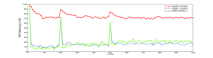
Figure 8: OSPA distance for linear and Gaussian scenario - The GM and CMC implementations widely outperform the classical SMC one because of the choice of the likelihood function $g_{n}({\mathbf{z}}|{\mathbf{x}})$.

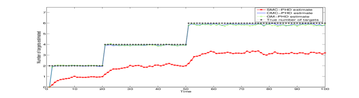
Figure 9: Estimator of the number of targets for linear and Gaussian scenario.

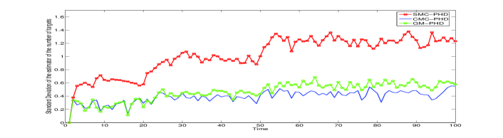
Figure 10: Standard Deviation of the estimator of the number of targets for linear and Gaussian scenario - The CMC estimator is slightly more reliable than the GM one when time increases.

5 Conclusion

In this paper we adapted CMC to single- and multi-object Bayesian filtering. In this framework, the recursive nature of SMC algorithms provides a conditioning variable at each time instant, but i.i.d. samples from this conditioning variable are unavailable. Our variance reduction method can be seen as a temporal, rather than spatial, RB-PF procedure; a Bayesian CMC estimator is ensured to outperform the associated crude MC one whatever the number of particles. We next showed that a CMC estimator can indeed be computed, or approximated, in a variety of Markovian stochastic models, including semi-linear HMC or JMSS, either at the same cost or at a reasonable extra computational cost. Finally we adapted Bayesian CMC to multi-target filtering, and showed that our CMC PHD filter has interesting practical features as compared to alternate (SMC or GM) implementations of the PHD filter. Our analysis was validated via simulations.

6 Aknowledgements

The authors would like to thank the French MOD DGA/MRIS for financial support of the Ph.D. of Y. Petetin.

References

- (1) A. Doucet, N. de Freitas, N. Gordon, Sequential Monte Carlo Methods in Practice, Statistics for Engineering and Information Science, Springer Verlag, New York, 2001.
- (2) M. S. Arulampalam, S. Maskell, N. Gordon, T. Clapp, A tutorial on particle filters for online nonlinear / non-Gaussian Bayesian tracking, IEEE Tr. Signal Processing 50 (2) (2002) 174–188.
- (3) R. Mahler, Multitarget Bayes filtering via first-order multitarget moments, IEEE Transactions on Aerospace and Electronic Systems 39 (4) (2003) 1152–1178.
- (4) S. Asmussen, P. W. Glynn, Stochastic Simulation: Algorithms and Analysis, Springer-Verlag, New York, NY, 2007.
- (5) R. Chen, J. S. Liu, Mixture Kalman filters, J. R. Statist. Soc. B 62 (2000) 493–508.
- (6) A. Doucet, S. J. Godsill, C. Andrieu, On sequential Monte Carlo sampling methods for Bayesian filtering, Statistics and Computing 10 (2000) 197–208.
- (7) A. Doucet, N. J. Gordon, V. Krishnamurthy, Particle filters for state estimation of jump Markov linear systems, IEEE Transactions on Signal Processing 49 (3) (2001) 613–24.
- (8) T. Schön, F. Gustafsson, P.-J. Nordlund, Marginalized particle filters for mixed linear nonlinear state-space models, IEEE Trans. on Signal Processing 53 (2005) 2279–2289.
- (9) J. Gewecke, Bayesian inference in econometric models using Monte Carlo integration, Econometrica 57 (6) (1989) 1317–1339.
- (10) N. Chopin, Central limit theorem for sequential Monte Carlo methods and its application to Bayesian inference, The Annals of Statistics 32 (6) (2004) 2385–2411.
- (11) F. Lindsten, T. Schön, J. Olsson, An explicit variance reduction expression for the Rao-Blackwellized particle filter, in: 18th World Congress of the Int. Federation of Automatic Control (IFAC), 2011.
- (12) D. B. Rubin, Using the SIR algorithm to simulate posterior distributions, in: M. H. Bernardo, K. M. Degroot, D. V. Lindley, A. F. M. Smith (Eds.), Bayesian Statistics III, Oxford University Press, Oxford, 1988.
- (13) A. E. Gelfand, A. F. M. Smith, Sampling based approaches to calculating marginal densities, Journal of the American Statistical Association 85 (410) (1990) 398–409.
- (14) A. F. M. Smith, A. E. Gelfand, Bayesian statistics without tears : a sampling-resampling perspective., The American Statistician 46 (2) (1992) 84–87.
- (15) V. Zaritskii, V. Svetnik, L. Shimelevich, Monte carlo techniques in problems of optimal data processing, Automation and remote control (1975) 95–103.
- (16) A. Kong, J. S. Liu, W. H. Wong, Sequential imputations and Bayesian missing data problems, Journal of the American Statistical Association 89 (425) (1994) 278–88.
- (17) J. S. Liu, R. Chen, Blind deconvolution via sequential imputation, Journal of the American Statistical Association 90 (430) (1995) 567–76.
- (18) S. Saha, P. K. Manda, Y. Boers, H. Driessen, A. Bagchi, Gaussian proposal density using moment matching in SMC methods., Statistics and Computing 19-2 (2009) 203–208.
- (19) S. Julier, J. Uhlmann, Unscented filtering and nonlinear estimation, in: Proceedings of the IEEE, Vol. 92, 2004, pp. 401–422.
- (20) M. K. Pitt, N. Shephard, Filtering via simulation : Auxiliary particle filters, Journal of the American Statistical Association 94 (446) (1999) 590–99.
- (21) P. Fearnhead, Computational methods for complex stochastic systems: A review of some alternatives to MCMC, Statistics and Computing 18 (2) (2008) 151–71.
- (22) A. M. Johansen, A. Doucet, A note on the auxiliary particle filter, Statistics and Probability Letters 78 (12) (2008) 1498–1504.
- (23) O. Cappé, É. Moulines, T. Rydén, Inference in Hidden Markov Models, Springer-Verlag, 2005.
- (24) N. J. Gordon, D. J. Salmond, A. F. M. Smith, Novel approach to nonlinear/ non-Gaussian Bayesian state estimation, IEE Proceedings-F 140 (2) (1993) 107–113.
- (25) J. K. Tugnait, Adaptive estimation and identification for discrete systems with Markov jump parameters, IEEE Transactions on Automatic Control 27 (5) (1982) 1054–65.
- (26) Y. Bar-Shalom, X. R. Li, T. Kirubarajan, Estimation with Applications to Tracking and Navigation, John Wiley and sons, New-York, 2001.
- (27) C. Musso, N. oudjane, F. LeGland, Improving regularised particle filters, in: A. Doucet, N. de Freitas, N. Gordon (Eds.), Sequential Monte Carlo Methods in Practice, Statistics for Engineering and Information Science, Springer Verlag, New York, 2001.
- (28) S. McGinnity, G. W. Irwin, Multiple model bootstrap filter for maneuvering target tracking, IEEE Transactions on Aerospace and Electronic Systems 36 (3) (2000) 1006–1012.
- (29) C. Andrieu, M. Davy, A. Doucet, Efficient Particle Filtering For Jump Markov Systems, IEEE trans. on Signal Processing 51 (2002) 1762–1770.
- (30) P. L’Ecuyer, Efficiency improvement and variance reduction, in: Winter Simulation Conference 1994, 1994, pp. 122–132.
- (31) Y. Bar-Shalom, Tracking and data association, Academic Press Professional, Inc., San Diego, CA, 1987.
- (32) S. Blackman, R. Popoli, Design and Analysis of Modern Tracking Systems, Artech House, 2009.
- (33) R. Mahler, Statistical Multisource Multitarget Information Fusion, Artech House, 2007.
- (34) B.-N. Vo, S. Singh, A. Doucet, Sequential Monte Carlo methods for multi-target filtering with random finite sets, IEEE Transactions on Aerospace and Electronic Systems 41.
- (35) B. Ristic, D. Clark, B. Vo, Improved SMC implementation of the PHD filter, in: Proceedings of the 13th International Conference on Information Fusion, 2010.
- (36) B.-N. Vo, W. Ma, The Gaussian mixture probability hypothesis density filter, IEEE Transactions on Signal Processing 54 (2006) 4091–4104.
- (37) D. Schuhmacher, B. T. Vo, B. N. Vo, A consistent metric for performance evaluation of multi-object filters, IEEE Transactions on Signal Processing 56 (8) (2008) 3447–3457.