Distilling one, two and entangled pairs of photons from a quantum dot with cavity QED effects and spectral filtering

Abstract

A quantum dot can be used as a source of one- and two-photon states and of polarisation entangled photon pairs. The emission of such states is investigated from the point of view of frequency-resolved two-photon correlations. These follow from a spectral filtering of the dot emission, which can be achieved either by using a cavity or by placing a number of interference filters before the detectors. The combination of these various options is used to iteratively refine the emission in a “distillation” process and arrive at highly correlated states with a high purity. So-called “leapfrog processes” where the system undergoes a direct transition from the biexciton state to the ground state by direct emission of two photons, are shown to be central to the quantum features of such sources. Optimum configurations are singled out in a global theoretical picture that unifies the various regimes of operation.

1 Introduction

Quantum dots have proven in the recent years to be excellent platforms for single photon sources [1, 2, 3], spin manipulation and coherent control at the exciton [4, 5, 6, 7, 8], or biexciton level [9, 10, 11, 12, 13, 14], or for entangled photon-pair generation [15, 16, 17]. The achievement of strong coupling between a single quantum dot and a cavity mode [18, 19, 20] impulsed even further these possibilities by increasing their efficiency and output-collectability [21, 22] to the point of reaching new regimes such as microlasing [23] or two-photon emission [24]. The cavity mode can also serve as a coupler between two distant dots [25, 26]. Cavity QED effects are thus a powerful resource to exploit the quantum features of a quantum dot [27, 28, 29, 30].

There is an alternative way to control, engineer and purify the emission of a quantum emitter which relies on extrinsic components at the macroscopic level, in contrast with the intrinsic approach at the microscopic level that supplements the quantum dot with a built-in microcavity. Namely, one can use spectral filtering. This approach is “extrinsic” in the sense that the filters are placed between the system which emits the light and the observer who detects it. As such, it belongs more properly with the detection part. The filter can in fact be modelling the finite resolution of a detector that is sensible only within a given frequency window. In this text, to keep the discussion as simple as possible, we will assume perfect detectors and describe the detection process through spectral filters (this means that the detector has a better resolution than the one imparted by the filter in front of it). Each filter is theoretically fully specified by its frequency of detection and linewidth. We will assume Lorentzian spectral shapes, which corresponds to the case of most interference filters. Commonly used spectral filter of this type are the thin-film filters and Fabry-Perot interferometers (in the figures, we will sketch such filters as dichroic bandpass filters, with different colours to imply different frequencies.) Since they rely on interference effects, they are basically cavities in weak coupling. This reinforces the main theme of this text which is to investigate cavity effects on a quantum emitter. The cavity itself can be, again, intrinsically part of the heterostructure itself, all packaged on-chip, or extrinsically due to the external filters. Combining these features, such as, filtering the emission of a cavity-QED system, we arrive to the notion of “distillation” where the emitter sees its output increasingly filtered by consecutive sequences to finally deliver a highly correlated quantum state of high purity.

While the idea is general and could be applied to a wealth of quantum emitters, we concentrate here on a single quantum dot, sketched as a little radiating pyramid in Fig. 1. Theoretically, it will be described as a combination of two two-level systems, representing two excitons of opposite spins. Such a system will be used for the generation of photons one by one or in pairs, with various types of quantum correlations. The four-level system formed by the two possible excitonic states (corresponding to orthogonal polarisations) and the doubly occupied state, the biexciton, is ideal to switch from one type of device to the other by simply selecting and enhancing the emission at the different intrinsic resonances [31, 32, 33]. Figure 1 gives a summary of the various filtering and detection schemes that will be applied, with the “naked” dot on the left. Its emission will be considered both from within or without a cavity, with various numbers of filters interceding. We will assume the microcavity both in the weak and strong-coupling regimes. The latter system has been extensively studied [31, 32, 33, 34, 35] and will be revisited here in the light of its spectral filtering [36] and distillation.

The rest of the text is organised as follows. In Sec. 2, we present the system and its basic properties and we introduce the two-photon spectrum which is the counterpart at the two-photon level of the photoluminescence spectrum at the single-photon one. In Sec. 3 we provide the first application of two-photon distillation, achieved via a cavity mode weakly coupled to the dot transitions or through spectral filtering. In Sec. 4, we compare the cavity filtering in the weak coupling regime with the enhancement of the emission in the strong coupling regime. In Sec. 4.1, we go one step further in the distillation of the two-photon emission and filter it from the cavity emission as well. In Sec. 5, we consider one of the most popular applications of the biexciton structure, the generation of polarisation entangled photon pairs. In Sec. 6 we draw some conclusions.

Figure 1: Sketch of the various schemes investigated in this text to study two-photon correlations from the light emitted by a quantum dot (left). The various detection configurations are, from left to right: 1, the direct emission of the dot ($g^{(2)}[\sigma_{\mathrm{H}}]$), 2, the enhanced and filtered emission of the dot by a cavity mode ($g^{(2)}[a]$); 3, the filtered emission of the dot ($g_{\Gamma}^{(2)}[\sigma_{\mathrm{H}}](\omega;\omega)$), 4, the two-photon spectroscopy of the dot ($g_{\Gamma}^{(2)}[\sigma_{\mathrm{H}}](\omega_{1};\omega_{2})$), 5, the filtered emission of the dot-in-a-cavity emission ($g_{\Gamma}^{(2)}[a](\omega;\omega)$), 6, the two-photon spectroscopy of the dot-in-a-cavity ($g_{\Gamma}^{(2)}[a](\omega_{1};\omega_{2})$) and 7, the tomographic reconstruction of the density matrix for the polarisation-entangled photon pairs, $\theta_{\Gamma}(\omega_{1},\omega_{2};\omega_{3},\omega_{4})$.

2 Two-photon spectrum from the quantum dot direct emission

The system under analysis consists of a quantum dot that can host up to two excitons with opposite spins. The corresponding orthogonal basis of linear polarisations, Horizontal (H) and Vertical (V), reads $\{\left|\mathrm{G}\right\rangle,\left|\mathrm{H}\right\rangle,\left|\mathrm{V}\right\rangle,\left|\mathrm{B}\right\rangle\}$, where G stands for the ground state, H and V for the single exciton states and B for the biexciton or doubly occupied state. The four level scheme that they form is depicted in Fig. 2(a). The Hamiltonian of the system reads ($\hbar=1$):

$$H_{\mathrm{dot}}=\Big{(}\omega_{\mathrm{X}}+\frac{\delta}{2}\Big{)}\left|\mathrm{H}\right\rangle\left\langle\mathrm{H}\right|+\Big{(}\omega_{\mathrm{X}}-\frac{\delta}{2}\Big{)}\left|\mathrm{V}\right\rangle\left\langle\mathrm{V}\right|+\omega_{\mathrm{B}}\left|\mathrm{B}\right\rangle\left\langle\mathrm{B}\right|\,,$$ (1)

where we allow the excitonic states to be split by a small energy $\delta$, as is typically the case experimentally, by the so-called fine structure splitting [24]. The biexciton at $\omega_{\mathrm{B}}=2\omega_{\mathrm{X}}-\chi$ is far detuned from twice the exciton thanks to the binding energy, $\chi$, typically the largest parameter in the system. We include the dot losses, at a rate $\gamma$, and an incoherent continuous excitation (off-resonant driving of the wetting layer), at a rate $P$, in both polarisations $x=$H, V, in a master equation:

$$\partial_{t}\rho=i[\rho,H_{\mathrm{dot}}]+\sum_{x\mathrm{=H,V}}\Big{[}\frac{\gamma}{2}\Big{(}\mathcal{L}_{\left|\mathrm{G}\right\rangle\left\langle x\right|}+\mathcal{L}_{\left|x\right\rangle\left\langle\mathrm{B}\right|}\Big{)}+\frac{P}{2}\Big{(}\mathcal{L}_{\left|x\right\rangle\left\langle\mathrm{G}\right|}+\mathcal{L}_{\left|\mathrm{B}\right\rangle\left\langle x\right|}\Big{)}\Big{]}(\rho)\,,$$ (2)

where $\mathcal{L}_{c}(\rho)=2c\rho c^{\dagger}-c^{\dagger}c\rho-\rho c^{\dagger}c$ is in the Lindblad form.

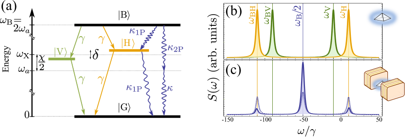
Figure 2: (a) Level scheme of the quantum dot investigated, modelled as a system able to accommodate two excitons $\left|\mathrm{V}\right\rangle$ and $\left|\mathrm{H}\right\rangle$ in the linear polarisation basis, with an energy splitting $\delta$ between them and which, when present jointly, form a biexciton $\left|\mathrm{B}\right\rangle$ with binding energy $\chi$. The excitons decay radiatively at a rate $\gamma$. When placed in a cavity (with linear polarisation H), two extra decay channels are opened for the H-polarisation: through the one-photon cascade at rate $\kappa_{\mathrm{1P}}$, and the two-photon emission at rate $\kappa_{\mathrm{2P}}$. In the sketch, the cavity is placed at the two-photon resonance $\omega_{a}=\omega_{\mathrm{B}}/2$. (b) PL spectra from the quantum dot system in H-polarisation (orange) consisting of two peaks at $\omega_{\mathrm{BH}}$ and $\omega_{\mathrm{H}}$, and in V-polarisation (green) consisting of two peaks at $\omega_{\mathrm{BV}}$ and $\omega_{\mathrm{V}}$. (c) PL spectrum when the dot is placed inside a cavity, both for the case of strong ($g=\kappa$, solid line) and weak ($g\rightarrow 0$, dotted line) coupling. A new peak appears at the centre from the two-photon emission. Parameters: $P=\gamma$, $\chi=100\gamma$, $\delta=20\gamma$, $\kappa=5\gamma$. We consider $\omega_{\mathrm{X}}\rightarrow 0$ as the reference frequency.

We assume in what follows an experimentally relevant situation, $\chi=100\gamma$, $\delta=20\gamma$, and study the steady state under $P=\gamma$, in which case all levels are equally populated (the populations read $\rho_{\mathrm{G}}=\gamma^{2}/(P+\gamma)^{2}$, $\rho_{\mathrm{H}}=\rho_{\mathrm{V}}=P\gamma/(P+\gamma)^{2}$ and $\rho_{\mathrm{B}}=P^{2}/(P+\gamma)^{2}$). The photoluminescence spectra of the system, $S(\omega)$, are shown in Fig. 2(b) for the H- and V-polarised emission with orange and green lines respectively. The four peaks are well separated thanks to the binding energy and fine structure splitting, corresponding to the four transitions depicted in panel (a) with the same colour code:

$$\omega_{\mathrm{BH}}=\omega_{\mathrm{B}}-\omega_{\mathrm{H}}=\omega_{\mathrm{X}}-\chi-\delta/2=-110\gamma\,,$$ (3)

$$\omega_{\mathrm{H}}=\omega_{\mathrm{X}}+\delta/2=10\gamma\,,$$ (4)

$$\omega_{\mathrm{BV}}=\omega_{\mathrm{B}}-\omega_{\mathrm{V}}=\omega_{\mathrm{X}}-\chi+\delta/2=-90\gamma\,,$$ (5)

$$\omega_{\mathrm{V}}=\omega_{\mathrm{X}}-\delta/2=-10\gamma\,,$$ (6)

with $\omega_{X}\rightarrow 0$ as the reference and FWHM $\gamma_{\mathrm{BH}}=\gamma_{\mathrm{BV}}=3\gamma+P$, $\gamma_{\mathrm{H}}=\gamma_{\mathrm{V}}=3P+\gamma$. We concentrate on the H-mode emission because it has the largest peak separation and allows for the best filtering but all results apply similarly to the V polarisation. The emission structure at the single-photon level is very simple: two Lorentzian peaks are observed corresponding to the upper and lower transitions,

$$S(\omega)=\frac{1}{\pi}\Big{[}\rho_{\mathrm{B}}\frac{\gamma_{\mathrm{BH}}/2}{(\gamma_{\mathrm{BH}}/2)^{2}+(\omega-\omega_{\mathrm{BH}})^{2}}+\rho_{\mathrm{H}}\frac{\gamma_{\mathrm{H}}/2}{(\gamma_{\mathrm{H}}/2)^{2}+(\omega-\omega_{\mathrm{H}})^{2}}\Big{]}\,.$$ (7)

The second-order coherence function of the H-emission in the steady state reads:

$$g^{(2)}[\sigma_{\mathrm{H}}](\tau)=\langle\sigma_{\mathrm{H}}^{+}(0)\sigma_{\mathrm{H}}^{+}(\tau)\sigma_{\mathrm{H}}(\tau)\sigma_{\mathrm{H}}(0)\rangle/\langle\sigma_{\mathrm{H}}^{+}\sigma_{\mathrm{H}}\rangle^{2}$$ (8)

where the H-photon destruction operator is defined as:

$$\sigma_{\mathrm{H}}=s_{1}+s_{2}\,,\quad\mathrm{with}\quad s_{1}=\left|\mathrm{H}\right\rangle\left\langle\mathrm{B}\right|\quad\mathrm{and}\quad s_{2}=\left|\mathrm{G}\right\rangle\left\langle\mathrm{H}\right|\,.$$ (9)

In Eq. (8), we have specified the channel of emission in square brackets since this will be an important attribute in the rest of the text. The quantum-dot described with the spin degree of freedom, exhibits uncorrelated statistics in the linear polarisation:

$$g^{(2)}[\sigma_{\mathrm{H}}](\tau)=1\,.$$ (10)

One recovers the expected antibunching of a two-level system [37], by turning to the intrinsic two-level systems composing the quantum dot, namely, the spin-up and spin-down excitons: $g^{(2)}[\sigma_{\uparrow}](0)=g^{(2)}[\sigma_{\downarrow}](0)=0$. The Pauli exclusion principle that holds for the spin $\sigma_{\updownarrows}$, breaks in the linear polarisation, i.e., while $\sigma_{\updownarrows}^{2}=0$, one has $\sigma_{\mathrm{H}}^{2}=\left|\mathrm{G}\right\rangle\left\langle\mathrm{B}\right|\neq 0$. We can find a simple explanation for this if we write the total correlations in terms of the four contributions (different from zero):

$$\langle\sigma_{\mathrm{H}}^{+}(0)\sigma_{\mathrm{H}}^{+}(\tau)\sigma_{\mathrm{H}}(\tau)\sigma_{\mathrm{H}}(0)\rangle=\sum_{i,j=1,2}\langle s_{i}^{+}(0)s_{j}^{+}(\tau)s_{j}(\tau)s_{i}(0)\rangle\,,$$ (11)

which are given by ($\tau\geq 0$):

$$g^{(2)}[s_{1};s_{1}](\tau)=(1-e^{-(\gamma+P)\tau})(1+\frac{\gamma}{P}e^{-(\gamma+P)\tau})\,,$$

$$g^{(2)}[s_{2};s_{2}](\tau)=(1-e^{-(\gamma+P)\tau})(1+\frac{P}{\gamma}e^{-(\gamma+P)\tau})\,,$$

$$g^{(2)}[s_{1};s_{2}](\tau)=(1-e^{-(\gamma+P)\tau})+e^{-(\gamma+P)\tau}(2+\frac{\gamma}{P}+\frac{P}{\gamma})\,,$$

$$g^{(2)}[s_{2};s_{1}](\tau)=(1-e^{-(\gamma+P)\tau})^{2}\,,$$ (12)

in their normalised form, $g^{(2)}[s_{i};s_{j}](\tau)=\langle s_{i}^{+}(0)s_{j}^{+}(\tau)s_{j}(\tau)s_{i}(0)\rangle/(\langle s_{i}^{+}s_{i}\rangle\langle s_{j}^{+}s_{j}\rangle)$. As shown in Fig. 3(c) and (d) with pale grey lines, all these functions are antibunched except for $g^{(2)}[s_{1};s_{2}](\tau)$, which corresponds to the natural order in the H-cascaded emission of two photons and is, consequently, bunched. It compensates fully the other three terms, leading to total correlations of 1 for all $\tau$.

Fig. 2 provides a clear picture o physical grounds of how such a system can be used as a quantum emitter but it lacks even a qualitative picture of how quantum correlations are distributed. Fig. 2(b) merely shows where the system emits light but nothing on how correlated is this emission. All these crucial features are revealed in the two-photon spectrum $g_{\Gamma}^{(2)}(\omega_{1};\omega_{2},\tau)$ [38]. This is the extension of the Glauber second order correlation function—which quantifies the correlations between photons in their arrival times—to frequency. By specifying both the energy and time of arrivals of the photons, one provides an essentially complete description of the system. $\Gamma$ denotes the linewidth of the frequency window of the filter over which this joint characterisation is obtained. The corresponding time-resolution is given by its inverse, $1/\Gamma$. It is a necessary variable without which nonsensical or trivial results are obtained.

The two-photon spectrum unravels a large class of processes hidden in single-photon spectroscopy and can be expected to become a standard tool to characterise and engineer quantum sources. The computation of such a quantity has remained a challenging task for theorists since the mid-eighties [39, 40, 41], until a recent workaround [36] has been found which allows an exact numerical computation. It will be applied here for the first time to the case of biexciton emission and used to understand, characterize and enhance various processes useful for its quantum emission. A detailed discussion on even more fundamental emitters is given in Ref. [38].

Experimentally, the two-photon spectrum corresponds to the usual Hanbury Brown–Twiss setup to measure second-order correlations through photon counting, with filters or monochromators being placed in front of the detectors to select two, in general different, frequency windows. The technique has been amply used in the laboratory [42, 43, 44, 45, 15, 16, 46, 22, 47, 48, 49] but lacking hitherto a general theoretical description, the global picture provided here has not yet been achieved experimentally. Note finally that when considering correlations between equal frequencies, $\omega_{1}=\omega_{2}$, the result is equivalent to placing a single filter before measuring the correlations of the outcoming photon stream [36].

Figure 3(a) shows the much richer landscape provided by the frequency resolved second-order coherence function, that is, the two-photon spectrum $g^{(2)}_{\Gamma}[\sigma_{\mathrm{H}}](\omega_{1};\omega_{2},\tau)$, in contrast with the one-photon spectrum $S(\omega)$ and the colour-blind second order correlations $g^{(2)}[\sigma_{\mathrm{H}}]$, Eq. (10). It is shown at zero delay ($\tau=0$) with the sensor linewidths taken to filter the full peaks ($\Gamma=5\gamma$). In such a case, one can see well defined regions of enhancement and suppression of the correlations: subpoissonian values ($<1$) are coloured in blue, Poissonian ($=1$) in white and superpoissonian ($>1$) in red. This figure is the backbone of this text. We now discuss in turns these different regions where the quantum-dot operates as a quantum source with different properties.

3 Distilling single photons and photon pairs

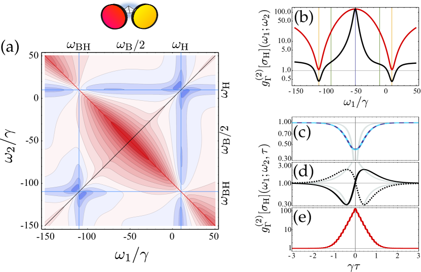
Figure 3: (a) Two-photon spectrum of a quantum dot (with a biexciton structure), with $\Gamma=5\gamma$. The density plot shows how the correlations between photons are distributed depending on their frequency of emission, from subpoissonian ($g_{\Gamma}^{2}[\sigma_{\mathrm{H}}](\omega_{1};\omega_{2})<1$, in blue) to superpoissonian ($>1$, in red) passing by Poissonian ($=1$, in white). The blue “butterflies” on the diagonal are typical of two-level systems. The antidiagonal corresponds to leapfrog processes with direct emission of two photons through an intermediate virtual state. (b) Cuts from the density plot along the diagonal $\omega_{2}=\omega_{1}$ (in black) and the antidiagonal $\omega_{2}=-\chi-\omega_{1}$ (in red). The diagonal also corresponds to applying a single filter. (c–e) Comparison of the $\tau$-dynamics for three cases of interest: (c) bunching at the heart of the two blue butterflies on the diagonal at $(\omega_{\mathrm{BH}};\omega_{\mathrm{BH}})$ (solid dark blue) and $(\omega_{\mathrm{H}};\omega_{\mathrm{H}})$ (dashed clear blue), (d) cross-correlation of the peaks at $(\omega_{\mathrm{BH}};\omega_{\mathrm{H}})$ (solid) and vice-versa, $(\omega_{\mathrm{H}};\omega_{\mathrm{BH}})$ (dotted), showing the typical cascade behaviour and (e) the strong bunching at $(\omega_{\mathrm{B}}/2;\omega_{\mathrm{b}}/2)$ where two-photon emission is optimum. In (c) and (d) we also plot with pale grey lines the second order correlations of the effective corresponding operators, Eqs. (2). All scales are logarithmic. Parameters: $P=\gamma$, $\chi=100\gamma$, $\delta=20\gamma$.

Single-photon source:

When the filters are tuned to the same frequency [diagonal black line in the $(\omega_{1};\omega_{2})$ space in Fig. 3(a)], there is a systematic enhancement of the bunching as compared to the surrounding regions due to the two possibilities of detecting identical photons [38]. Despite this feature, that is independent of the system dynamics, when both frequencies coincide with one of the dot transitions, $(\omega_{\mathrm{H}};\omega_{\mathrm{H}})$ or $(\omega_{\mathrm{BH}};\omega_{\mathrm{BH}})$, there is a dip in the correlations. This is more clearly shown in the cut at equal frequencies, the black line in Fig. 3(b). The blue butterfly shape that is observed in the two-photon spectrum locally around each of the dot transitions is characteristic of an isolated two-level system [38]. This zero delay information is complemented by the antibunched $\tau$ dynamics, shown in Fig. 3(c). The two dot resonances, upper and lower, coincide in this case due to the symmetric conditions $P=\gamma$ but they are typically different (the upper level being less antibunched at low pump). Filtering and detection makes impossible to have a perfect antibunching, getting closest to the ideal correlations $g_{\Gamma}^{(2)}[\sigma_{\mathrm{H}}](\omega_{\mathrm{H}};\omega_{\mathrm{H}},\tau)\approx g^{(2)}[s_{1};s_{1}](\tau)$ from Eqs. (2), at around $\Gamma\approx\chi/2$. At this point, the peaks are maximally filtered with still negligible overlapping of the filters. It is possible to derive a useful expression for the filtered correlations at $\tau=0$, with $\Gamma\leq\chi/2$, in the limit:

$$\lim_{\chi\rightarrow\infty}g_{\Gamma}^{(2)}[\sigma_{\mathrm{H}}](\omega_{\mathrm{H}};\omega_{\mathrm{H}})=\frac{2(P+\gamma)^{2}(3P+\gamma+\Gamma)(2\gamma+\Gamma)}{\gamma(P+\gamma+\Gamma)(2P+2\gamma+\Gamma)(3P+\gamma+3\Gamma)}\,,$$ (13)

typically relevant in experiments.

All this shows that one can recover or optimise the quantum features of a single photon source (antibunching) in a system whose total emission is uncorrelated, by frequency filtering photons from individual transitions. Consequently, the system should exhibit two-photon blockade when probed by a resonant laser at frequency $\omega_{\mathrm{L}}$ in resonance with the lower transition, $\omega_{\mathrm{L}}=\omega_{\mathrm{H}}$. The antibunched emission of each of the four filtered peaks of the spectrum, has been observed experimentally [15].

Cascaded two-photon emission:

When the filtering frequencies match both the upper and lower quantum dot transitions, i.e., $(\omega_{\mathrm{BH}};\omega_{\mathrm{H}})$, the correlations are close to one at zero delay, like for the total emission $g^{(2)}[\sigma_{\mathrm{H}}]$ (which is exactly one). However, although the latter is uncorrelated, since it remains equal to one at all $\tau$, the filtered cascade emission is not uncorrelated since it is close to unity only at zero delay and precisely because of strong correlations that are, however, of an opposite nature at positive and negative delays, i.e., showing enhancement for $\tau>0$ when photons are detected in the natural order that they are emitted, and suppression for $\tau<0$ when the order is the opposite. This is depicted in Fig. 3(d) where the solid line corresponds to $(\omega_{\mathrm{BH}};\omega_{\mathrm{H}})$ and the dotted line to exchanging the filters, $(\omega_{\mathrm{H}};\omega_{\mathrm{BH}})$. As this also corresponds to detecting the photons in the opposite time order, the two curves are exact mirror image of each other.

The identification of the upper and lower transition photons with frequency-blind operators [$g^{(2)}[s_{1};s_{2}](\tau)$ in Eqs. (2)] provides crossed correlations different to our exact and general frequency resolved functions, specially at $\tau=0$, as shown in Fig. 3(d), where there is a discontinuity for the approximated functions. The frequency resolved functions have the typical smooth cascade shape that been observed experimentally [45, 15]. The dynamics at large $\tau$, converges to the approximated functions only for $\Gamma\approx\chi/2$.

Simultaneous two-photon emission:

For simultaneous two-photon emission, the strongest feature lies on the antidiagonal (red line) in Fig. 3(a), which is also shown as the solid red line in Fig. 3(b). The strong bunching observed here, when both frequencies are far from the system resonances $\omega_{\mathrm{BH}}$ and $\omega_{\mathrm{H}}$, corresponds to a two-photon deexcitation directly from the biexciton to the ground state without passing by an intermediate real state. This two-photon emission from a Hamiltonian, Eq. (1), that does not have a term to describe such a process is made possible via a virtual state that arises in the quantum dynamics and that can be revealed by the spectral filtering. As the intermediate virtual state has no fixed energy and only the total energy $\omega_{1}+\omega_{2}=\omega_{\mathrm{B}}$ needs be conserved, the simultaneous two-photon emission is observed on the entire antidiagonal (except, again, when touching a resonance, in which case the cascade through real states takes over). We call such processes “leapfrog” as they jump over the intermediate excitonic state [38]. The largest bunching is found at the central point, $\omega_{1}=\omega_{2}=\omega_{\mathrm{B}}/2=-\chi/2$, and at the far-ends $\omega_{1}\ll\omega_{\mathrm{BH}}$ and $\omega_{1}\gg\omega_{\mathrm{H}}$. Among them, the optimal point is that where also the intensity of the two-photon emission is strong. The frequency resolved Mandel $Q$ parameter takes into account both correlations and the strength of the filtered signal [50]:

$$Q_{\Gamma}(\omega_{1};\omega_{2})=\sqrt{S_{\Gamma}(\omega_{1})S_{\Gamma}(\omega_{2})}\Big{[}g^{(2)}_{\Gamma}(\omega_{1};\omega_{2})-1\Big{]}$$ (14)

(where also for the single-photon spectra, the detection linewidth, $\Gamma$, is taken into account [51]). As expected, $Q_{\Gamma}[\sigma_{\mathrm{H}}](\omega_{1};\omega_{2})$ becomes negligible at very large frequencies, far from the resonances of the system, and reaches its maximum at the two-photon resonance, $(\omega_{\mathrm{B}}/2;\omega_{\mathrm{B}}/2)$ (not shown). This latter configuration is therefore the best candidate for the simultaneous and, additionally, indistinguishable, emission of two photons. The bunching is shown in Fig. 3(e). The small and fast oscillations are due to the effect of one-photon dynamics with the real states but are unimportant for our discussion and would be difficult to resolve experimentally. While the bunching in such a configuration has not yet been observed experimentally, recently, Ota et al. successfully filtered the two-photon emission from the biexciton with a cavity mode [24], which corroborates the above discussion.

4 Filtering and enhancing photon-pair emission from the quantum dot via a cavity mode

Large two-photon correlations are the starting point to create a two-photon emission device. When they have been identified, the next step is to increase their efficiency by enhancing the emission at the right operational frequency. The typical way is to Purcell enhance the emission through a cavity mode with the adequate polarisation and strongly coupled with the dot transitions (at resonance). Theoretically this amounts to adding to the master equation (2) a Hamiltonian part, that accounts for the free cavity mode ($\omega_{a}$) and the coupling to the dot (with strength $g$),

$$H_{\mathrm{cav}}=\omega_{a}a^{\dagger}a+g(a^{\dagger}\sigma_{\mathrm{H}}+a\sigma_{\mathrm{H}}^{\dagger})\,,$$ (15)

along with a Lindblad term $\frac{\kappa}{2}\mathcal{L}_{a}(\rho)$, that accounts for the cavity decay (at rate $\kappa$).

By placing the cavity mode at the two-photon resonance, $\omega_{a}=\omega_{\mathrm{B}}/2$, the virtual leapfrog process becomes real as it finds a real intermediate state in the form of a cavity photon. The deexcitation of the biexciton to ground state is thereby enhanced at a rate $\kappa_{\mathrm{2PR}}\approx(4g^{2}/\chi)^{2}/\kappa$, producing the emission of two simultaneous and indistinguishable cavity photons at this frequency [31, 32, 33]. There is as well some probability that the cavity mediated deexcitation occurs in two steps, through two different cavity photons at frequencies $\omega_{\mathrm{BH}}$ and $\omega_{\mathrm{H}}$, at the same rate $\kappa_{\mathrm{1PR}}\approx 4g^{2}\kappa/\chi^{2}$. The two alternative paths are schematically depicted with curly blue arrows in Fig. 2(a). The cavity being far from resonance with the dot transitions, the ratio of two- versus one-photon emission can be controlled by an appropriate choice of parameters [32]. We set $g=\kappa=5\gamma$, to be in strong coupling regime and have $\kappa_{\mathrm{2P}}=0.2\gamma>\kappa_{\mathrm{1P}}=0.05\gamma$, but with a coupling weak enough for the system to emit cavity photons efficiently. The cavity parameters are such that $\kappa>2P$ and the pump does not disrupt the two-photon dynamics [33]. The two-photon emission indeed dominates over the one-photon emission as seen in Fig. 2(c), where the cavity spectrum is plotted with a solid line: the central peak, corresponding to the simultaneous two-photon emission, is more intense than the side peaks produced by single photons. A better cavity (smaller $\kappa$) does not emit the biexciton photons right away outside of the system, but spoils the original (leapfrog) correlations and leads to smaller correlations in the cavity emission $g^{(2)}[a]=\langle a^{\dagger}a^{\dagger}aa\rangle/\langle a^{\dagger}a\rangle^{2}\rightarrow 2$. This is shown in Fig. 4(a) with a blue solid line. Our previous choice $\kappa=5\gamma$, is close to that which maximises bunching (vertical line in Fig. 4(a)). A weak coupling due to small coupling strength ($g\rightarrow 0$), plotted with a blue dotted line, recovers the case of a filter, discussed in the previous Section. The cavity spectrum in this case, plotted with a blue dotted line in Fig. 2(c), is no longer dominated by the two-photon emission.

Regardless of the coupling strength $g$, the system goes into weak-coupling at large enough $\kappa$, so both blue lines, solid and dotted, converge to the same curve at $\kappa\rightarrow\infty$. The cavity then filters the whole dot emission and recovers the total dot correlations for the H-mode, $g^{(2)}[a]\rightarrow g^{(2)}[\sigma_{\mathrm{H}}]=1$. Note that while the bunching in $g^{(2)}[a]$ is better in weak-coupling or with a filter, this is at the price of decreasing the enhancement of the emission and, therefore, the efficiency of the quantum device, as the total Mandel $Q[a]$ parameter shows in Fig. 4(b).

4.1 Distilling the two-photon emission from the cavity field

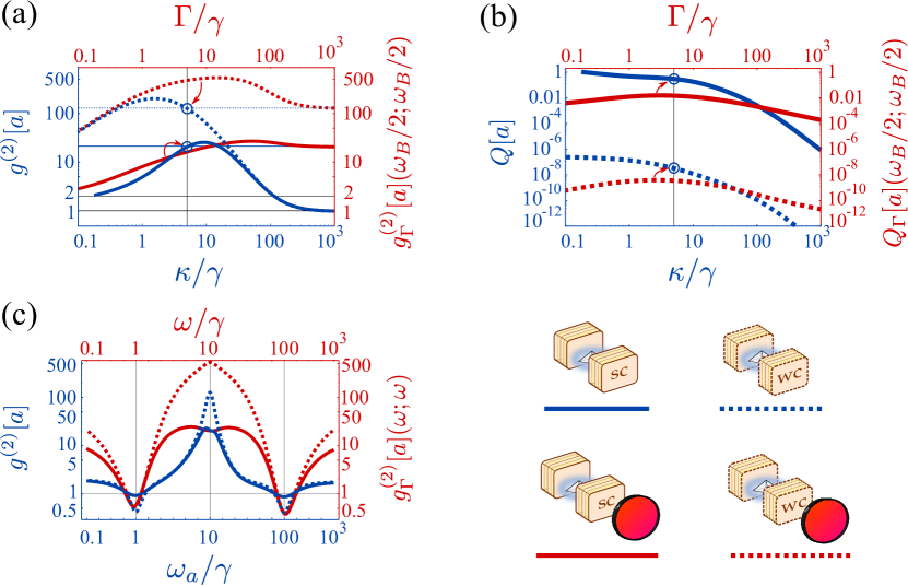
Figure 4: (a) Second order correlations of a cavity mode embedding a quantum dot in weak (dotted) and strong (solid) coupling. Both the full, colour-blind, cavity emission (in blue) $g^{(2)}[a]$ and the frequency-resolved correlations at the two-photon resonance (in red) $g^{(2)}_{\Gamma}[a](\omega_{\mathrm{B}}/2;\omega_{\mathrm{B}}/2)$ are considered, with the former relating to the bottom axis (the cavity linewidth $\kappa$) and the latter to the upper axis (the detector linewidth $\Gamma$) at $\kappa=5\gamma$ (indicated by a circle). (b) Mandel $Q$ parameter in the same configuration as in (a), supplementing the information of the previous panel with the intensity of the emission. (c) Same as (a) but now as a function of the cavity frequency $\omega_{a}$ (bottom axis) for the colour-blind correlations (in blue) and of the detection frequency $\omega$ (upper axis) for the frequency-resolved correlations. Parameters: (a) the strong coupling is for $g=5\gamma$ and the weak coupling is in the limit of vanishing coupling $g\rightarrow 0$ where the cavity is fully equivalent to a filter. Parameters: $P=\gamma$, $\chi=100\gamma$, $\delta=20\gamma$.

In view of the preceding results, we now consider the possibility to further enhance the two-photon emission by filtering the cavity photons from the central peak in Fig. 2(c). That is, we study $g_{\Gamma}^{(2)}[a](\omega_{1};\omega_{2})$ for a cavity with $\kappa=5\gamma$ and $\omega_{a}=\omega_{\mathrm{B}}/2$. In this way, first, the cavity acts as a filter, extracting the leapfrog emission where it is most correlated, but also enhances specifically the two-photon emission and, second, the filtering of the cavity emission selects only those photons that truly come in pairs. Such a chain is alike to a “distillation” process where the quantum emission is successively refined.

The results are plotted with red lines in Fig. 4, for the case $\kappa=5g$ pinpointed by circles on the blue lines. The filtered cavity emission is indeed generally more strongly correlated at the two-photon resonance than the unfiltered total cavity emission, plotted in blue: $g_{\Gamma}^{(2)}[a](\omega_{\mathrm{B}}/2;\omega_{\mathrm{B}}/2)\geq g^{(2)}[a]$. This is so for all $\Gamma>\kappa$ for the cavity in weak-coupling, where the distillation always enhances the correlations. In strong coupling, the filter must strongly overlap with the peak ($\Gamma\gg\kappa$). This is because the side peaks are prominent in weak-coupling ($\kappa_{\mathrm{2P}}<\kappa_{\mathrm{1P}}$), and the filtering efficiently suppress their detrimental effect, whereas in strong-coupling, two-photon correlations are already close to maximum thanks to the dominant central peak as seen in Fig. 2(c), and it is therefore important for the filter to strongly overlap with it. In all cases, at large enough $\Gamma$, the full cavity correlations are recovered as expected: $\lim_{\Gamma\rightarrow\infty}g_{\Gamma}^{(2)}[a](\omega_{1};\omega_{2})=g^{(2)}[a]$. In Fig. 4(a), this means that the red lines converge to the value projected by the circle on the blue lines at $\kappa=5\gamma$. Here, again, filtering enhances correlations but reduces the number of counts, as shown in Fig. 4(b).

In Fig. 4(c), we do the same analysis as in Fig. 3(b) where there was no distillation. We address the same cases but now as a function of frequency, fixing the cavity decay rate $\kappa=5\gamma$ and the filtering linewidth at $\Gamma=10\gamma$. In blue, we consider the cavity QED case in weak- and strong-coupling, without filtering. Since the weak-coupling limit is identical to the single filter case, note that the blue dotted line in Fig. 4(c) is identical to the black solid line in Fig. 3(b). Off-resonance, the cavity acts as a simple filter due to the reduction of the effective coupling. The stronger coupling to the cavity has an effect only when involving the real states, where it spoils the correlations, less bunched at the two-photon resonance $\omega_{a}=\omega_{\mathrm{B}}/2$, and less antibunched at the one-photon resonances, $\omega_{a}=\omega_{\mathrm{BH}}$ or $\omega_{a}=\omega_{\mathrm{H}}$. This shows again that useful quantum correlations are obtained in a system where quantum processes are Purcell enhanced and quickly transferred outside, rather than stored and Rabi-cycled over within the cavity. The same is true for the red line, further filtering the output. Finally, comparing solid lines together, we see again that there is little if anything to be gained by filtering in strong-coupling, whereas in weak-coupling, the enhancement is considerable. As a summary, the filtering of the weakly coupled cavity (red dotted), provides the strongest correlations (at the cost of the available intensity), corresponding to distilling the photon pairs out of the original dot spectrum without any additional enhancement.

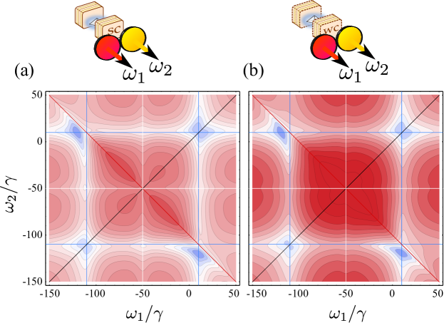
Figure 5: Two-photon spectra $g^{(2)}_{\Gamma}[a](\omega_{1};\omega_{2})$ for a quantum dot in a cavity in the (a) strong, $g=\kappa$, and (b) weak coupling regime, when the cavity is at the two-photon resonance, $\omega_{a}=\omega_{\mathrm{B}}/2$. The bunching regions are strengthened by the cavity (the total, colour-blind correlations are $g^{(2)}[a]\approx 21$). A horizontal and vertical structure also emerges at the two-photon resonance, betraying the emergence of real states. These are stronger the stronger the coupling. The same logarithmic scale as Fig. 3(a) applies, so all three figures can be compared directly. Parameters: $\kappa=5\gamma$, $P=\gamma$, $\chi=100\gamma$, $\delta=20\gamma$ and $\Gamma=10\kappa$.

In Fig. 5, we show the full two-photon spectra for a quantum dot in a cavity, in both (a) strong- and (b) weak-coupling. The same colour code and logarithmic scale is used as in Fig. 3(a), for comparison. The antibunching regions on the diagonal and the bunching ones on the antidiagonal are qualitatively similar to the filtered dot emission, but antibunching is milder and less extended while correlations are, respectively, weaker (stronger) at the central point due to the saturated (efficient) distillation in strong (weak) coupling. Another striking feature added by the cavity is the appearance of an additional pattern of horizontal and vertical lines at $\omega_{a}=\omega_{\mathrm{B}}/2$. While diagonal and anti-diagonal features correspond to virtual processes, horizontal and vertical stem from real processes, that pin the correlations at their own frequency. Therefore, the new features are a further illustration that the two-photon emission becomes a real resonance of the cavity-dot system, in contrast with Fig. 3(a) where it was virtual. The effect is more pronounced in the strong-coupling regime since this is the case where the new state is better defined. Another qualitative difference between Fig. 5 and Fig. 3(a) is in the regions surrounding the cascade configuration, $(\omega_{\mathrm{BH}};\omega_{\mathrm{H}})$, which has changed shape around two antibunching spots. This is due to the fact that the single-photon cascade is much less likely to happen through the cavity mode than the direct deexcitation of the dot, as $\kappa_{\mathrm{1P}}=0.05\gamma\ll\gamma$. Even if the first photon from the biexciton emission decays through the cavity, the second will most likely not. This new two antibunching spots are slightly pushed to the left of the red line by the leapfrog bunching line and the presence of the V-polarised resonances.

5 Distilling entangled photon pairs

One of the most sophisticated applications of the biexciton structure in a quantum dot is as a source of polarisation entangled photon pairs [52, 15, 16, 53, 54, 55, 56, 57, 58, 21, 59, 60, 35, 61]. Without the fine-structure splitting, $\delta=0$, the two possible two-photon deexcitation paths are indistinguishable except for their polarisation degree of freedom (H or V), producing equal frequency photon pairs $(\omega_{\mathrm{BX}};\omega_{\mathrm{X}})$, with $\omega_{\mathrm{BX}}=\omega_{\mathrm{B}}-\omega_{\mathrm{X}}$. This results in the polarisation entangled state:

$$\left|\psi\right\rangle=\frac{1}{\sqrt{2}}\left(\left|\mathrm{H(\omega_{\mathrm{BX}}),H(\omega_{\mathrm{X}})}\right\rangle+e^{-i\phi}\left|\mathrm{V(\omega_{\mathrm{BX}}),V(\omega_{\mathrm{X}})}\right\rangle\right)\,.$$ (16)

The splitting $\delta$ provides “which path” information [62] that spoils indistinguishability, producing a state entangled in both frequency and polarisation [34]:

$$\left|\psi^{\prime}\right\rangle=\frac{1}{\sqrt{2}}\left(\left|\mathrm{H(\omega_{\mathrm{BH}}),H(\omega_{\mathrm{H}})}\right\rangle+e^{-i\phi^{\prime}}\left|\mathrm{V(\omega_{\mathrm{BV}}),V(\omega_{\mathrm{V}})}\right\rangle\right)\,.$$ (17)

Although these doubly entangled states are useful for some quantum applications [63, 64], it is typically desirable to erase the frequency information and recover polarisation-only entangled pairs. Among other solutions, such as canceling the built-in splitting externally [16, 65], filtering has been implemented with $\omega_{1}=\omega_{\mathrm{BX}}$ and $\omega_{2}=\omega_{\mathrm{X}}$ to make the pairs identical in frequencies again [34, 15, 54], at the cost of increasing the randomness of the source (making it less “on-demand”). Recently, the cavity filtering of the polarisation entangled photon pairs with $\omega_{a}=\omega_{\mathrm{B}}/2$ has been proposed by Schumacher et al. [35], taking advantage of the additional two-photon enhancement [32]. Let us revisit these effects in the light of the previous results.

The properties of the output photons can be obtained from the two-photon state density matrix, $\theta(\tau)$, reconstructed in the basis $\{\left|\mathrm{H1,H2}\right\rangle,\left|\mathrm{H1,V4}\right\rangle,\left|\mathrm{V3,H2}\right\rangle,\left|\mathrm{V3,V4}\right\rangle\}$, denoting by $\left|xi\right\rangle$ with $x=$H or V and $i=1,2,3,4$, the state $\left|x(\omega_{i})\right\rangle$. The frequencies $\omega_{i}$ are, in general, different. The second photon is detected with a delay $\tau$ with respect to the first one (detected in the steady state). Let us express this matrix in terms of frequency resolved correlators, as is typically done in the literature [53, 55]. However, in contrast to previous approaches, we do not identify the photons with the transition from which they may come from (using the dot operators $\left|\mathrm{G}\right\rangle\left\langle x\right|$, $\left|x\right\rangle\left\langle\mathrm{B}\right|$ with, again, $x$ standing for either H or V) but with their measurable properties, that is, polarisation, frequency and time of detection (for a given filter window). This is a more accurate description of the experimental situation where a given photon can come from any dot transition and any transition can produce photons at any frequency and time with some probability. We describe the experiments by considering four different filters, that is, including all degrees of freedom of the emitted photons in the description. Each detected filtered photon corresponds to the application of the filter operator $\varsigma_{j}$ with $j=$H1, H2, V3, V4 corresponding to its coupling to the H or V dot transitions with $\omega_{i}$ frequencies. Then, the two-photon matrix $\theta^{\prime}_{\Gamma}(\tau)$ (the prime refers to the lack of normalisation) corresponding to a tomographic measurement is theoretically modelled as:

$$\theta_{\Gamma}^{\prime}(\tau)=\left(\begin{array}[]{cccc}\langle n_{\mathrm{H1}}(0)n_{\mathrm{H2}}(\tau)\rangle&\langle n_{\mathrm{H1}}(0)[\varsigma_{\mathrm{H2}}^{+}\varsigma_{\mathrm{V4}}](\tau)\rangle&\langle[\varsigma_{\mathrm{H1}}^{+}\varsigma_{\mathrm{V3}}](0)n_{\mathrm{H2}}(\tau)\rangle\\ \mathrm{h.c.}&\langle n_{\mathrm{H1}}(0)n_{\mathrm{V4}}(\tau)\rangle&\langle[\varsigma_{\mathrm{H1}}^{+}\varsigma_{\mathrm{V3}}](0)[\varsigma_{\mathrm{V4}}^{+}\varsigma_{\mathrm{H2}}](\tau)\rangle\\ \mathrm{h.c.}&\mathrm{h.c.}&\langle n_{\mathrm{V3}}(0)n_{\mathrm{H2}}(\tau)\rangle\\ \mathrm{h.c.}&\mathrm{h.c.}&\mathrm{h.c.}\end{array}\right.$$ (22)

$$\hskip 206.28247pt\left.\begin{array}[]{c}\langle[\varsigma_{\mathrm{H1}}^{+}\varsigma_{\mathrm{V3}}](0)[\varsigma_{\mathrm{H2}}^{+}\varsigma_{\mathrm{V4}}](\tau)\rangle\\ \langle[\varsigma_{\mathrm{H1}}^{+}\varsigma_{\mathrm{V3}}](0)n_{\mathrm{V4}}(\tau)\rangle\\ \langle n_{\mathrm{V3}}(0)[\varsigma_{\mathrm{H2}}^{+}\varsigma_{\mathrm{V4}}](\tau)\rangle\\ \langle n_{\mathrm{V3}}(0)n_{\mathrm{V4}}(\tau)\rangle\end{array}\right)\,,$$ (27)

where $n_{i}=\varsigma_{i}^{+}\varsigma_{i}$ [we have dropped the frequency dependence in the notation, writing $\theta_{\Gamma}^{\prime}(\tau)$ instead of $\theta_{\Gamma}^{\prime}(\omega_{1},\omega_{2};\omega_{3},\omega_{4},\tau)$]. Since a weakly coupled cavity mode behaves as a filter, this tomographic procedure is equivalent to considering the four dot transitions coupled to four different cavity modes with the corresponding polarisations, central frequencies and decay rates [35, 61]. Unlike in other works where for various reasons and particular cases, some of the elements in $\theta_{\Gamma}^{\prime}(\tau)$ are set to zero or considered equal, here we keep the full matrix with no a priori assumptions since, in general, it may not reduce to a simpler form due to the incoherent pumping, pure dephasing, frequency filtering and fine-structure splitting.

There are essentially two ways to quantify the degree of entanglement from the density matrix $\theta_{\Gamma}^{\prime}(\tau)$. The most straightforward is to consider the $\tau$-dependent matrix directly, which merely requires normalisation at each time $\tau$, yielding $\theta_{\Gamma}(\tau)=\theta_{\Gamma}^{\prime}(\tau)/\mathrm{Tr}[\theta_{\Gamma}^{\prime}(\tau)]$. The physical interpretation is that of photon pairs emitted with a delay $\tau$, that is to say, within the time-resolution $1/\Gamma$ of the filter or cavity [34, 61]. In particular, the zero-delay matrix, $\theta_{\Gamma}(0)$, represents the emission of two simultaneous photons [59, 60]. The second approach is closer to the experimental measurement which averages over time. In this case, one considers the integrated quantity $\Theta_{\Gamma}(\tau_{\mathrm{max}})=\big{(}\int_{0}^{\tau_{\mathrm{max}}}\theta_{\Gamma}^{\prime}(\tau)\,d\tau\big{)}/\mathcal{N}$, that averages over all possible emitted pairs from the system [15, 53]. It is also normalised (by $\mathcal{N}$), but after integration, so that the two approaches are not directly related to each other and present alternative aspects of the problem, discussed in detail in the following. Without the cutoff delay $\tau_{\mathrm{max}}$, the integral diverges due to the continuous pumping.

The degree of entanglement of any bipartite system represented by a $4\times 4$ density matrix $\theta$, can be quantified by the concurrence, $C$, which ranges from 0 (separable states) to 1 (maximally entangled states) [66]. High values of the concurrence require high degrees of purity in the system [67], being, for instance, impossible to extract any entanglement from a maximally mixed state (in which case all the four basis states occur with the same probability). The filtered density matrices, $\Theta_{\Gamma}(\tau_{\mathrm{max}})$ and $\theta_{\Gamma}(\tau)$, provide each their own concurrence that we will denote $C_{\Gamma}^{\mathrm{int}}(\tau_{\mathrm{max}})$ and $C_{\Gamma}(\tau)$, respectively.

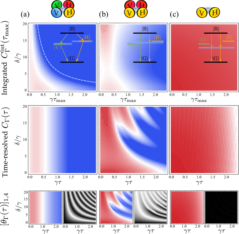
Figure 6: Concurrence for three different schemes of entanglement distillation (as sketched above each column): (a) filtering the four different dot resonances in their cascade through the real states, (b) filtering at two different frequencies $\omega_{1}=\omega_{\mathrm{BX}}$ and $\omega_{2}=\omega_{\mathrm{X}}$, degenerate in both polarisation decay paths, (c) filtering at the same frequency $\omega_{\mathrm{B}}/2$, i.e., at the two-photon resonance. The upper panels show the time-integrated concurrence $C_{\Gamma}^{\mathrm{int}}(\tau_{\mathrm{max}})$ as a function of its cutoff $\tau_{\mathrm{max}}$ and the fine-structure splitting $\delta$. In (a) the line $\tau_{\mathrm{max}}=2\pi/\delta$ bounding the region with entanglement is superimposed. The intermediate panels show the instantaneous concurrence $C_{\Gamma}(\tau)$ as a function of delay and splitting. The lowest panels show the modulus and phase of the off-diagonal element $[\theta_{\Gamma}(\tau)]_{1,4}$ typically used in the literature to quantify entanglement. All these plots show that as far as the degree of entanglement is concerned, the leapfrog emission is the best configuration and is optimum at the two-photon resonance. The concurrence colour code is blue for 0, white for 0.5 and red for 1. In the modulus density plots, the colour code is blue for 0, white for 0.25 and red for values $\geq 0.5$. In the phase density plots, the colour code is black for values approaching $-\pi$ and white for $\pi$. Parameters: $P=\gamma$, $\chi=100\gamma$, $\Gamma=2\gamma$.

We begin by considering the standard cascade configuration by detecting photons at the dot resonances, i.e., $\omega_{1}=\omega_{\mathrm{BH}}$, $\omega_{2}=\omega_{\mathrm{H}}$, $\omega_{3}=\omega_{\mathrm{BV}}$, $\omega_{4}=\omega_{\mathrm{V}}$, as sketched in the inset of Fig. 6(a). The upper density plot shows $C_{\Gamma}^{\mathrm{int}}(\tau_{\mathrm{max}})$ and the density plot below shows the time-resolved concurrence $C_{\Gamma}(\tau)$, as a function of $\tau_{\mathrm{max}}$ or $\tau$ and $\delta$, for $\Gamma=2\gamma$. The two concurrences, $C_{\Gamma}^{\mathrm{int}}(\tau_{\mathrm{max}})$ and $C_{\Gamma}(\tau)$, are qualitatively different except at $\tau=\tau_{\mathrm{max}}=0$ where they are equal by definition. They also have in common that the maximum concurrence is not achieved at zero delay [it is most visible as the darker red area around $(\gamma\tau_{\mathrm{max}},\delta/\gamma)\approx(0.4,0)$]. This is because this filtering scheme relies on the real-states deexcitation of the dot levels, and thus exhibits the typical delay from the cascade-type dynamics of correlations [see Fig. 3(d)]. The major departure between the two is that the decay of $C^{\mathrm{int}}_{\Gamma}(\tau_{\mathrm{max}})$ is strongly dependent on $\delta$, while $C_{\Gamma}(\tau)$ is not. With no splitting, at $\delta=0$, the ideal symmetrical four-level structure efficiently produces the entangled state $\left|\psi\right\rangle$ and the concurrence is maximum both for the integral and the time-resolved forms. The decay time of $C_{\Gamma}(\tau)$ is the simplest to understand as, when filtering full peaks, it is merely related to the reloading time of the biexciton, of the order of the inverse pumping rate, $\sim 2/P$ [61]. The asymmetry due to a nonzero splitting in the four-level system causes an unbalanced dynamics of deexcitation via the H and V polarisations. The entanglement in the form $\left|\psi\right\rangle$ is downgraded to $\left|\psi^{\prime}\right\rangle$. The fact that the concurrence $C_{\Gamma}(\tau)$ is not affected shows that it accounts for the degree of entanglement in both polarisation and frequency, which is oblivious to the “which path” information that the last variable provides. On the other hand, $C_{\Gamma}^{\mathrm{int}}(\tau_{\mathrm{max}})$ is suppressed by the splitting as fast as $\tau_{\mathrm{max}}>2\pi/\delta$ (this boundary is superimposed to the density plot). That is, as soon as the integration interval is large enough to resolve it. The integrated $C_{\Gamma}^{\mathrm{int}}(\tau_{\mathrm{max}})$, therefore, accounts for the degree of entanglement in polarisation only, and is destroyed by the “which path” information provided by the different frequencies. The exact mechanism at work to erase the entanglement is shown in the lower row of Fig. 6, which displays the upper right matrix element $[\theta_{\Gamma}(\tau)]_{1,4}$ of the density matrix, that is the most responsible for purporting entanglement. The modulus is shown on the left (with blue meaning 0 and red meaning $\geq 0.5$) and the phase on the right (in black and white). The time-resolved concurrence $C_{\Gamma}(\tau)$ is very similar to the modulus of $[\theta_{\Gamma}(\tau)]_{1,4}$ which justifies the approximation often-made in the literature $C_{\Gamma}(\tau)=2(|[\theta_{\Gamma}(\tau)]_{1,4}|-[\theta_{\Gamma}(\tau)]_{2,2})$ with $[\theta_{\Gamma}(\tau)]_{2,2}$ small [53]. Although each photon pair is entangled, it is so in the state $\left|\psi^{\prime}\right\rangle$ with a phase, $\phi^{\prime}=-\pi+\delta\tau$, that accumulates with $\tau$ at a rate $\delta$ [34], but this does not matter as far as instantaneous entanglement is concerned, and this is why the splitting does not affect $C_{\Gamma}(\tau)$. On the other hand, when integrating over time, the varying phase, that completes a $2\pi$-cycle at intervals $2\pi/\delta$, randomises the quantum superposition and results in a classical mixture. This is why the splitting does completely destroy $C_{\Gamma}^{\mathrm{int}}(\tau_{\mathrm{max}})$ for $\tau_{\mathrm{max}}>2\pi/\delta$. And this is how the system restores the “which path” information: given enough time, if the splitting is large enough, the photons loose their quantum coherence due to the averaging out of the relative phase between them because of their distinguishable frequency.

Another possible configuration proposed in the literature [34, 15, 54] is sketched in the inset of Fig. 6(b). Photons are detected at the frequency that lies between the two polarisations, $\omega_{1}=\omega_{3}=\omega_{\mathrm{BX}}$, $\omega_{2}=\omega_{4}=\omega_{\mathrm{X}}$. For small splittings, the entanglement production scheme still relies on the cascade and real deexcitation of the dot levels. Therefore, the behaviour of $C_{\Gamma}^{\mathrm{int}}(\tau_{\mathrm{max}})$ is similar to (a) (decaying with $\delta$) but slightly improved by the fact that the contributions to the density matrix are more balanced by filtering in-between the levels. For splittings large enough to allow the formation of leapfrog emission in both paths, $\delta\gg\Gamma$, there is a striking change of trend and $C_{\Gamma}^{\mathrm{int}}(\tau_{\mathrm{max}})$ remains finite at longer delays $\tau_{\mathrm{max}}$ when increasing $\delta$. This is a clear sign that the entanglement relies on a different type of emission, namely simultaneous leapfrog photon pairs, rather than a cascade through real states. Accordingly, the intensity is reduced as compared to that obtained at smaller $\delta$ or to the non-degenerate cascade in (a), but the bunching is stronger, as evidenced by the two-photon spectrum, and results in a larger degree of entanglement than at $\delta=0$. A similar result is obtained qualitatively with the time-resolved concurrence, a strong resurgence of entanglement with $\delta$, indicating again very high correlations in this configuration. Note finally that the phase becomes much more constant with increasing $\delta$, resulting in the persistence of the correlation in the time-integrated concurrence. This is because the two-photon emission is through the leapfrog processes. Since the latter, by definition, involve intermediate virtual states that are degenerate in frequency, this is a built-in mechanism to suppress the splitting and not suffer from the “which path” information as when passing through the real states.

Finally, a configuration proposed more recently in the literature [35] is the two-photon resonance, with four equal frequencies, $\omega_{1}=\omega_{2}=\omega_{3}=\omega_{4}=\omega_{\mathrm{B}}/2$, as sketched in the inset of Fig. 6(c). This provides a two-photon source in both polarisations that can be enhanced via two cavity modes with orthogonal polarisations [32]. Remarkably, in this case, the splitting has almost no effect on the degree of entanglement, that is maximum. Here, the leapfrog mechanism plays at its full extent: the virtual states, on top of being degenerated and thus immune to the splitting, remain always far, and are therefore protected, from the real states. This results in the exactly constant phase (black panel on the lower right end of Fig. 6). As a result, both $C_{\Gamma}^{\mathrm{int}}(\tau_{\mathrm{max}})$ and $C_{\Gamma}(\tau)$ remain large. The only drawback of this mechanism is, being virtual-processes mediated, a comparatively weaker intensity.

We conclude with a more detailed analysis of what appears to be the most suitable scheme to create a robust entanglement, the leapfrog photon-pair emission. The target state is always $\left|\psi\right\rangle$, Eq. (16), due to the degeneracy in the filtered paths. The concurrence is shown as a function of the first photon frequency, $\omega_{1}$, in Fig. 7 (the second photon has the energy $\omega_{2}=\omega_{\mathrm{B}}-\omega_{1}$ to conserve the total biexciton energy). The time-integrated (resp. instantaneous) concurrence $C_{\Gamma}^{\mathrm{int}}(1/\gamma)$ [resp. $C_{\Gamma}(0)$] is shown in red (resp. blue) lines, both for a large splitting $\delta=20\gamma$ in strong tones and for $\delta=0$ in softer tones. In the first panel, (a), the frequency $\omega_{1}$ of the filters are varied. This figure shows that concurrence is very high (with high state purity) when the filtering frequencies are far from the system resonances: $\omega_{\mathrm{BH/BV}}$ and $\omega_{\mathrm{H/V}}$. These are shown as coloured grid lines to guide the eye. In this case, the real states are not involved and the leapfrog emission is efficient in both polarisations. The concurrence otherwise drops down when $\omega_{1}$ is resonant with any one-photon transition, meaning that photons are then emitted in a cascade in one of the polarisations, rather than simultaneously through a leapfrog process. Moreover, if at least one of the two deexcitation paths is dominated by the real state dynamics, this brings back the problem of “which path” information, that spoils indistinguishability and entanglement. There is only one exception to this general rule, namely, the $\delta=0$ integrated case (soft red line) which has a local maximum at $\omega_{\mathrm{BX}}$, i.e., when touching its resonance in the natural cascade order. This is because the paths are anyway identical and the integration includes the possibility of emitting the second photon with some delay (up to $\tau_{\mathrm{max}}$). For the case of $\delta\neq 0$, if this is large enough, it is still possible to recover identical paths while filtering the leapfrog in the middle points, $\omega_{1}=\omega_{\mathrm{BX}}$ and $\omega_{2}=\omega_{\mathrm{X}}$, to produce entangled pairs.

Overall, the optimum configuration is, therefore, indeed at the middle point $\omega_{1}=\omega_{2}=\omega_{\mathrm{B}}/2$ (two-photon resonance), where the photons are emitted simultaneously, with a high purity, and entanglement degrees are also identical in frequency by construction. Entanglement is also always larger in the simultaneous concurrence (blue lines) as this is the natural choice to detect the leapfrog emission, which is a fast process. This comes at the price, expectedly, of decreasing the total number of useful counts and increasing the randomness of the source. Note finally that the blue curves are symmetric around $\omega_{\mathrm{B}}/2$, but the red ones are not, given that in the integrated case, the order of the photons with different frequencies is relevant. The left-hand side of the plot, $\omega_{1}<\omega_{\mathrm{B}}/2$, corresponds to the natural order of the frequencies in the cascade, $\omega_{1}<\omega_{2}$. The opposite order, being counter-decay, is detrimental for entanglement.

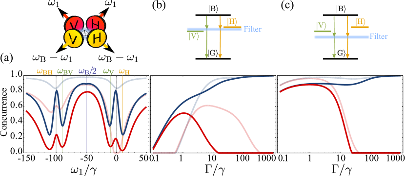
Figure 7: Concurrence computed with the instantaneous emission at $\tau=0$ (blue) or integrated up to $\tau_{\mathrm{max}}=1/\gamma$ (red). (a) Plotted for a fixed filter linewidth $\Gamma=5\gamma$ as a function of the filters frequencies $(\omega_{1};\omega_{\mathrm{B}}-\omega_{1})$. The concurrence is high unless a real state is probed and a cascade through it overtakes the leapfrog emission. The optimum case is the two-photon resonance. (b–c) Plotted as a function of the filter linewidth $\Gamma$ for the two cases that maximise entanglement in (a), that is at (b) the degenerate cascade configuration $(\omega_{\mathrm{BX}};\omega_{\mathrm{X}})$ and (c) the biexciton two-photon resonance $(\omega_{\mathrm{B}}/2;\omega_{\mathrm{B}}/2)$. The concurrence of the ideal case at $\delta=0$ is also plotted as a reference with softer solid lines. Parameters: $P=\gamma$, $\chi=100\gamma$, $\delta=20\gamma$. $\omega_{\mathrm{X}}=0$ is set as the reference frequency.

Of all leapfrog configurations, those in panels (b) and (c) of Fig. 6 are therefore the optimum cases to obtain high degrees of entanglement. Let us conclude with a study on their dependence on the filter linewidths, $\Gamma$, in Figs. 7(b) and (c). First, we observe that in the limit of small linewidths for the filters, i.e., in the region $\Gamma<1/\tau_{\mathrm{max}}$, the simultaneous and time-integrated concurrences should converge to each other, since the time resolution becomes larger than the integration time. Therefore, the integrated emission provides the maximum entanglement when the frequency window is small enough to provide the same results than the simultaneous emission. Decreasing $\Gamma$ below $P$ (which in this case is also $P=\gamma$) results in a time resolution in the filtering larger than the pumping timescale $1/P$. Therefore, photons from different pumping cycles start to get mixed with each others. As a result $C$ drops for $\Gamma<\gamma$ in all cases. In the limit $\Gamma\ll P$, the emission is completely uncorrelated and $C=0$. This is an important difference from the cases of pulsed excitation or the spontaneous decay of the system from the biexciton state. In the absence of a steady state, entanglement is maximised with the smallest window, $\Gamma\rightarrow 0$ [15, 54]. Two opposite behaviours are otherwise observed in these figures when increasing the filter linewidth and $\Gamma>1/\tau_{\mathrm{max}}$. The simultaneous emission gains in its degree of entanglement whereas the time-integrated one loses with increasing linewidth. In the limit $\Gamma\rightarrow\infty$, this disparity is easy to understand. We recover the colour blind result in all filtering configurations, (b) or (c), that is, the decay of entanglement: from 1 corresponding to $\left|\psi\right\rangle$ at $\tau=0$, to 0 corresponding to a maximally mixed state at large $\tau$. Therefore, $C_{\Gamma}(0)\rightarrow C(0)=1$ and $C_{\Gamma}^{\mathrm{int}}(\tau_{\mathrm{max}})\rightarrow C^{\mathrm{int}}(\tau_{\mathrm{max}})=0$ (for our particular choice of $\tau_{\mathrm{max}}$ and $P$).

The decrease in $C_{\Gamma}^{\mathrm{int}}(\tau_{\mathrm{max}})$ when increasing the filtering window, has been discussed in the literature for the case in Fig. 7(b) [15, 54], and it has been attributed to a gain of “which path” information due to the overlap of the filters with the real excitonic levels. In the lights of our results, when $\Gamma>\delta$ the real state deexcitation takes over the leapfrog and $C_{\Gamma}^{\mathrm{int}}(\tau_{\mathrm{max}})$ is suppressed indeed due to such a gain of “which path” information, as discussed previously. However, we find another reason why $C_{\Gamma}^{\mathrm{int}}(\tau_{\mathrm{max}})$ decreases with $\Gamma$ in all cases, based on the leapfrog emission: the region $1/P<\Gamma<\delta$ for case (b) and the region $1/P<\Gamma<\chi$ for case (c). The maximum delay in the emission of the second photon in a leapfrog processes is related to $1/\Gamma$, due to its virtual nature. Therefore, the initial enhancement of entanglement starts to drop at delays $\tau\approx 1/\Gamma$, after which the emission of a second photon is uncorrelated to the first one (not belonging to the same leapfrog pair). For a fixed cutoff $\tau_{\mathrm{max}}$, this leads to a reduction of $C_{\Gamma}^{\mathrm{int}}(\tau_{\mathrm{max}})$ with $\Gamma$. Broader filters have a smaller impact on the case of real state deexcitation [see the zero splitting case in Fig. 7(b), plotted in soft red]: since the system dynamics is slower than the filtering ($\gamma$, $P<\Gamma$), the filter merely emits the photons faster and faster after receiving them from the system. This results in a mild reduction of $C_{\Gamma}^{\mathrm{int}}(\tau_{\mathrm{max}})$ with $\Gamma$ until the detection becomes colour blind and it drops to reach its aforementioned limit of zero.

6 Conclusions

In summary, we have characterised the emission of a quantum dot modelled as a system able to accommodate two excitons of different polarisation and bound as a biexciton. Beyond the usual single-photon spectrum (or photoluminescence spectrum), we have presented for the first time the two-photon spectrum of such a system, and discussed the physical processes unravelled by frequency-resolved correlations and how they shed light on various mechanisms useful for quantum information processing.

We relied on the recently developed formalism [36] that allows to compute conveniently such correlations resolved both in time and frequency. This describes both the application of external filters before the detection or due to one or many cavity modes in weak-coupling with the emitter. Filters and cavities have their respective advantages, and when combined, can realize a distillation of the emission, by successive filtering that enhance the correlations and purity of the states.

We addressed three different regimes of operation depending on the filtering scheme, namely as a source of single photons, a source of two-photon states (both through cascaded photon pairs and simultaneous photon pairs) and as a source of polarisation entangled photon pairs, for which a form of the density matrix that is close to the experimental tomographic procedure was proposed. In particular, so-called leapfrog processes—where the system undergoes a direct transition from the biexciton to the ground state without passing by the intermediate real states but jumping over them through a virtual state—have been identified as key, both for two-photon emission and for entangled photon-pair generation. In the latter case, this allows to cancel the notoriously detrimental splitting between the real exciton states that spoils entanglement through a “which path” information, since the intermediate virtual states have no energy constrains and are always perfectly degenerate. Entanglement is long-lived and much more robust against this splitting than when filtering at the system resonances. At the two-photon resonance, degrees of entanglement higher than $80\%$ can be achieved and maintained for a wide range of parameters.

References

References

- [1] S. Strauf, N. G. Stoltz, M. T. Rakher, L. A. Coldren, P. M. Petroff, and D. Bouwmeester. High-frequency single-photon source with polarization control. Nat. Photon., 1:704, 2007.
- [2] H. S. Nguyen, G. Sallen, C. Voisin, Ph. Roussignol, C. Diederichs, and G. Cassabois. Ultra-coherent single photon source. Appl. Phys. Lett., 99:261904, 2011.
- [3] C. Matthiesen, A. N. Vamivakas, and M. Atatüre. Subnatural linewidth single photons from a quantum dot. Phys. Rev. Lett., 108:093602, 2012.
- [4] S. J. Boyle, A. J. Ramsay, A. M. Fox, and M. S. Skolnick. Beating of exciton-dressed states in a single semiconductor InGaAs/GaAs quantum dot. Phys. Rev. Lett., 102:207401, 2009.
- [5] A. N. Vamivakas, Y. Zhao, C.-Y. Lu, and M. Atatüre. Spin-resolved quantum-dot resonance fluorescence. Nat. Phys., 5:198, 2009.
- [6] A. J. Ramsay. A review of the coherent optical control of the exciton and spin states of semiconductor quantum dots. Semicond. Sci. Technol., 25:103001, 2010.
- [7] C. M. Simon, T. Belhadj, B. Chatel, T. Amand, P. Renucci, A. Lemaitre, O. Krebs, P. A. Dalgarno, R. J. Warburton, X. Marie, and B. Urbaszek. Robust quantum dot exciton generation via adiabatic passage with frequency-swept optical pulses. Phys. Rev. Lett., 106:166801, 2011.
- [8] Yanwen Wu, I. M. Piper, M. Ediger, P. Brereton, E. R. Schmidgall, P. R. Eastham, M. Hugues, M. Hopkinson, and R. T. Phillips. Population inversion in a single InGaAs quantum dot using the method of adiabatic rapid passage. Phys. Rev. Lett., 106:067401, 2011.
- [9] G. Chen, T. H. Stievater, E. T. Batteh, X. Li, D. G. Steel, D. Gammon, D. S. Katzer, D. Park, and L. J. Sham. Biexciton quantum coherence in a single quantum dot. Phys. Rev. Lett., 88:117901, 2002.
- [10] T. Flissikowski, A. Betke, I. A. Akimov, and F. Henneberger. Two-photon coherent control of a single quantum dot. Phys. Rev. Lett., 92:227401, 2004.
- [11] S. Stufler, P. Machnikowski, P. Ester, M. Bichler, V. M. Axt, T. Kuhn, and A. Zrenner. Two-photon Rabi oscillations in a single InxGa1-xAs/GaAs quantum dot. Phys. Rev. B, 73:125304, 2006.
- [12] I. A. Akimov, J. T. Andrews, and F. Henneberger. Stimulated emission from the biexciton in a single self-assembled II-VI quantum dot. Phys. Rev. Lett., 96:067401, 2006.
- [13] S.J. Boyle, A.J. Ramsay, , A.M. Fox, and M.S. Skolnick. Two-color two-photon rabi oscillation of biexciton in single InAs/GaAs quantum dot. Physica E, 42:2485, 2010.
- [14] T. Miyazawa, T. Kodera, T. Nakaoka, K. Watanabe, N. Kumagai, N. Yokoyama, and Y. Arakawa. Two-photon control of biexciton population in telecommunication-band quantum dot. Appl. Phys. Express, 3:064401, 2010.
- [15] N. Akopian, N. H. Lindner, E. Poem, Y. Berlatzky, J. Avron, D. Gershoni, B. D. Gerardot, and P. M. Petroff. Entangled photon pairs from semiconductor quantum dots. Phys. Rev. Lett., 96:130501, 2006.
- [16] R. M. Stevenson, R. J. Young, P. Atkinson, K. Cooper, D. A. Ritchie, and A. J. Shields. A semiconductor source of triggered entangled photon pairs. Nature, 439:179, 2006.
- [17] R. Hafenbrak, S. M. Ulrich, P. Michler, L. Wang, A. Rastelli, and O. G. Schmidt. Triggered polarization-entangled photon pairs from a single quantum dot up to 30K. New J. Phys., 9:315, 2007.
- [18] J. P. Reithmaier, G. Sek, A. Löffler, C. Hofmann, S. Kuhn, S. Reitzenstein, L. V. Keldysh, V. D. Kulakovskii, T. L. Reinecker, and A. Forchel. Strong coupling in a single quantum dot–semiconductor microcavity system. Nature, 432:197, 2004.
- [19] T. Yoshie, A. Scherer, J. Heindrickson, G. Khitrova, H. M. Gibbs, G. Rupper, C. Ell, O. B. Shchekin, and D. G. Deppe. Vacuum Rabi splitting with a single quantum dot in a photonic crystal nanocavity. Nature, 432:200, 2004.
- [20] E. Peter, P. Senellart, D. Martrou, A. Lemaître, J. Hours, J. M. Gérard, and J. Bloch. Exciton-photon strong-coupling regime for a single quantum dot embedded in a microcavity. Phys. Rev. Lett., 95:067401, 2005.
- [21] A. Dousse, J. Suffczyński, A. Beveratos, O. Krebs, A. Lemaître, I. Sagnes, J. Bloch, P. Voisin, and P. Senellart. Ultrabright source of entangled photon pairs. Nature, 466:217, 2010.
- [22] K. Hennessy, A. Badolato, M. Winger, D. Gerace, M. Atature, S. Gulde, S. Fălt, E. L. Hu, and A. Ĭmamoḡlu. Quantum nature of a strongly coupled single quantum dot–cavity system. Nature, 445:896, 2007.
- [23] M. Nomura, N. Kumagai, S. Iwamoto, Y. Ota, and Y. Arakawa. Laser oscillation in a strongly coupled single-quantum-dot–nanocavity system. Nat. Phys., 6:279, 2010.
- [24] Y. Ota, S. Iwamoto, N. Kumagai, and Y. Arakawa. Spontaneous two-photon emission from a single quantum dot. Phys. Rev. Lett., 107:233602, 2011.
- [25] A. Laucht, J.M. Villas-Bôas, S. Stobbe, N. Hauke, F. Hofbauer, G. Böhm, P. Lodahl, M.-C. Amannand, M. Kaniber, and J. J. Finley. Mutual coupling of two semiconductor quantum dots via an optical nanocavity. Phys. Rev. B, 82:075305, 2010.
- [26] E. Gallardo, L. J. Martinez, A. K. Nowak, D. Sarkar, H. P. van der Meulen, J. M. Calleja, C. Tejedor, I. Prieto, D. Granados, A. G. Taboada, J. M. García, and P. A. Postigo. Optical coupling of two distant InAs/GaAs quantum dots by a photonic-crystal microcavity. Phys. Rev. B, 81:193301, 2010.
- [27] L. Schneebeli, M. Kira, and S. W. Koch. Characterization of strong light–matter coupling in semiconductor quantum-dot microcavities via photon-statistics spectroscopy. Phys. Rev. Lett., 101:097401, 2008.
- [28] J. Kasprzak, S. Reitzenstein, E. A. Muljarov, C. Kistner, C. Schneider, M. Strauss, S. Höfling, A. Forchel, and W. Langbein. Up on the Jaynes-Cummings ladder of a quantum-dot/microcavity system. Nat. Mater., 9:304, 2010.
- [29] F.P. Laussy, E. del Valle, M. Schrapp, A. Laucht, and J. J. Finley. Climbing the Jaynes–Cummings ladder by photon counting. arXiv:1104.3564, 2011.
- [30] A. Majumdar, M. Bajcsy, and J. Vuckovic. Probing the ladder of dressed states and nonclassical light generation in quantum-dot–cavity QED. Phys. Rev. A, 85:041801(R), 2012.
- [31] E. del Valle, S. Zippilli, F. P. Laussy, A. Gonzalez-Tudela, G. Morigi, and C. Tejedor. Two-photon lasing by a single quantum dot in a high- microcavity. Phys. Rev. B, 81:035302, 2010.
- [32] E. del Valle, A. Gonzalez-Tudela, E. Cancellieri, F. P. Laussy, and C. Tejedor. Generation of a two-photon state from a quantum dot in a microcavity. New J. Phys., 13:113014, 2011.
- [33] E. del Valle, A. Gonzalez-Tudela, and F. P. Laussy. Generation of a two-photon state from a quantum dot in a microcavity under incoherent and coherent continuous excitation. Proc. SPIE, 8255:825505, 2012.
- [34] T. M. Stace, G. J. Milburn, and C. H. W. Barnes. Entangled two-photon source using biexciton emission of an asymmetric quantum dot in a cavity. Phys. Rev. B, 67:085317, 2003.
- [35] S. Schumacher, J. Förstner, A. Zrenner, M. Florian, C. Gies, P. Gartner, and F. Jahnke. Cavity-assisted emission of polarization-entangled photons from biexcitons in quantum dots with fine-structure splitting. Opt. Express, 20:5335, 2012.
- [36] E. del Valle, A. Gonzalez-Tudela, F. P. Laussy, C. Tejedor, and M. J. Hartmann. Theory of frequency-filtered and time-resolved -photon correlations. Phys. Rev. Lett., 109:183601, 2012.
- [37] B. R. Mollow. Power spectrum of light scattered by two-level systems. Phys. Rev., 188:1969, 1969.
- [38] A. Gonzalez-Tudela, F. P. Laussy, C. Tejedor, M J. Hartmann, and E. del Valle. Two-photon spectra of quantum emitters. In preparation., 2012.
- [39] H. F. Arnoldus and G. Nienhuis. Photon correlations between the lines in the spectrum of resonance fluorescence. J. phys. B.: At. Mol. Phys., 17:963, 1984.
- [40] L. Knöll and G. Weber. Theory of -fold time-resolved correlation spectroscopy and its application to resonance fluorescence radiation. J. phys. B.: At. Mol. Phys., 19:2817, 1986.
- [41] J. D. Cresser. Intensity correlations of frequency-filtered light fields. J. phys. B.: At. Mol. Phys., 20:4915, 1987.
- [42] A. Aspect, G. Roger, S. Reynaud, J. Dalibard, and C. Cohen-Tannoudji. Time correlations between the two sidebands of the resonance fluorescence triplet. Phys. Rev. Lett., 45:617, 1980.
- [43] C. A. Schrama, G. Nienhuis, H. A. Dijkerman, C. Steijsiger, and H. G. M. Heideman. Destructive interference between opposite time orders of photon emission. Phys. Rev. Lett., 67, 1991.
- [44] R. Centeno Neelen, D. M. Boersma, M. P. van Exter, G. Nienhuis, and J. P. Woerdman. Spectral filtering within the Schawlow–Townes linewidth as a diagnostic tool for studying laser phase noise. Opt. Commun., 100:289, 1993.
- [45] E. Moreau, I. Robert, L. Manin, V. Thierry-Mieg, J. M. Gérard, and I. Abram. Quantum cascade of photons in semiconductor quantum dots. Phys. Rev. Lett., 87:183601, 2001.
- [46] D. Press, S. Götzinger, S. Reitzenstein, C. Hofmann, A. Löffler, M. Kamp, A. Forchel, and Y. Yamamoto. Photon antibunching from a single quantum dot-microcavity system in the strong coupling regime. Phys. Rev. Lett., 98:117402, 2007.
- [47] M. Kaniber, A. Laucht, A. Neumann, J. M. Villas-Bôas, M. Bichler, M.-C. Amann, and J. J. Finley. Investigation of the nonresonant dot-cavity coupling in two-dimensional photonic crystal nanocavities. Phys. Rev. B, 77:161303(R), 2008.
- [48] G. Sallen, A. Tribu, T. Aichele, R. André, L. Besombes, C. Bougerol, M. Richard, S. Tatarenko, K. Kheng, and J.-Ph. Poizat. Subnanosecond spectral diffusion measurement using photon correlation. Nat. Photon., 4:696, 2010.
- [49] A. Ulhaq, S. Weiler, S. M. Ulrich, R. Roßbach, M. Jetter, and P. Michler. Cascaded single-photon emission from the Mollow triplet sidebands of a quantum dot. Nat. Photon., 6:238, 2012.
- [50] G. Bel and F. L. H. Brown. Theory for wavelength-resolved photon emission statistics in single-molecule fluorescence spectroscopy. Phys. Rev. Lett., 102:018303, 2009.
- [51] J.H. Eberly and K. Wódkiewicz. The time-dependent physical spectrum of light. J. Opt. Soc. Am., 67:1252, 1977.
- [52] O. Benson, C. Santori, M. Pelton, and Y. Yamamoto. Regulated and entangled photons from a single quantum dot. Phys. Rev. Lett., 84:2513, 2000.
- [53] F. Troiani, J. I. Perea, and C. Tejedor. Analysis of the photon indistinguishability in incoherently excited quantum dots. Phys. Rev. B, 73:035316, 2006.
- [54] E. A. Meirom, N. H. Lindner, Y. Berlatzky, E. Poem, N. Akopian, J. E. Avron, and D. Gershoni. Distilling entanglement from random cascades with partial “which path” ambiguity. Phys. Rev. A, 77:062310, 2008.
- [55] G. Pfanner, M. Seliger, and U. Hohenester. Entangled photon sources based on semiconductor quantum dots: The role of pure dephasing. Phys. Rev. B, 78:195410, 2008.
- [56] J. E. Avron, G. Bisker, D. Gershoni, N. H. Lindner, E. A. Meirom, and R. J. Warburton. Entanglement on demand through time reordering. Phys. Rev. Lett., 100:120501, 2008.
- [57] R. Johne, N. A. Gippius, G. Pavlovic, D. D. Solnyshkov, I. A. Shelykh, and G. Malpuech. Entangled photon pairs produced by a quantum dot strongly coupled to a microcavity. Phys. Rev. Lett., 100:240404, 2008.
- [58] P. K. Pathak and S. Hughes. Generation of entangled photon pairs from a single quantum dot embedded in a planar photonic-crystal cavity. Phys. Rev. B, 79:205416, 2009.
- [59] A. Carmele, F. Milde, M.-R. Dachner, M. B. Harouni, R. Roknizadeh, M. Richter, and A. Knorr. Formation dynamics of an entangled photon pair: A temperature-dependent analysis. Phys. Rev. B, 81:195319, 2010.
- [60] A. Carmele and A. Knorr. Analytical solution of the quantum-state tomography of the biexciton cascade in semiconductor quantum dots: Pure dephasing does not affect entanglement. Phys. Rev. B, 84:075328, 2011.
- [61] A. N. Poddubny. Effect of continuous and pulsed pumping on entangled photon pair generation in semiconductor microcavities. Phys. Rev. B, 85:075311, 2012.
- [62] M. O. Scully, B.-G. Englert, and H. Walther. Quantum optical tests of complementarity. Nature, 351:111, 1991.
- [63] W. Chuan and Z. Yong. Quantum secret sharing protocol using modulated doubly entangled photons. Chinese Phys., 18:3238, 2009.
- [64] H. Wang, S. Liu, and J. He. Thermal entanglement in two-atom cavity QED and the entangled quantum otto engine. Phys. Rev. E, 79:041113, 2009.
- [65] R. Trotta, E. Zallo, C. Ortix, P. Atkinson, J. D. Plumhof, J. van den Brink, A. Rastelli1, and O. G. Schmid. Universal recovery of the energy-level degeneracy of bright excitons in ingaas quantum dots without a structure symmetry. Phys. Rev. Lett., 109:147401, 2012.
- [66] W. K. Wootters. Entanglement of formation of an arbitrary state of two qubits. Phys. Rev. Lett., 80:2245, 1998.
- [67] W. J. Munro, D. F. V. James, A. G. White, and P. G. Kwiat. Maximizing the entanglement of two mixed qubits. Phys. Rev. A, 64:030302, 2001.