“$L=R$” – $U(1)_{R}$ Lepton Number at the LHC

Abstract

We perform a detailed study of a variety of LHC signals in supersymmetric models where lepton number is promoted to an (approximate) $U(1)_{R}$ symmetry. Such a symmetry has interesting implications for naturalness, as well as flavor- and CP-violation, among others. Interestingly, it makes large sneutrino vacuum expectation values phenomenologically viable, so that a slepton doublet can play the role of the down-type Higgs. As a result, (some of) the leptons and neutrinos are incorporated into the chargino and neutralino sectors. This leads to characteristic decay patterns that can be experimentally tested at the LHC. The corresponding collider phenomenology is largely determined by the new approximately conserved quantum number, which is itself closely tied to the presence of “leptonic R-parity violation”. We find rather loose bounds on the first and second generation squarks, arising from a combination of suppressed production rates together with relatively small signal efficiencies of the current searches. Naturalness would indicate that such a framework should be discovered in the near future, perhaps through spectacular signals exhibiting the lepto-quark nature of the third generation squarks. The presence of fully visible decays, in addition to decay chains involving large missing energy (in the form of neutrinos) could give handles to access the details of the spectrum of new particles, if excesses over SM background were to be observed. The scale of neutrino masses is intimately tied to the source of $U(1)_{R}$ breaking, thus opening a window into the $R$-breaking sector through neutrino physics. Further theoretical aspects of the model have been presented in the companion paper [1].

1 Introduction

The recent discovery at the LHC of a Higgs-like signal at $\sim 125~{}{\rm GeV}$ has put the general issue of electroweak symmetry breaking under a renewed perspective. In addition, the absence of other new physics signals is rapidly constraining a number of theoretically well-motivated scenarios. One of these concerns supersymmetry, which in its minimal version is being tested already above the TeV scale. In view of this, it is pertinent to consider alternate realizations that could allow our prejudices regarding e.g. naturalness to be consistent with the current experimental landscape, within a supersymmetric framework. At the same time, such scenarios might motivate studies for non-standard new physics signals.

One such non-standard realization of supersymmetry involves the possible existence of an approximately conserved $R$-symmetry at the electroweak scale [2, 3, 4, 5, 6, 7, 8, 9, 10, 11, 12, 13]. It is known that one of the characteristics of such scenarios, namely the Dirac character of the gauginos (in particular, gluinos), can significantly soften the current exclusion bounds [14, 15]. At the same time, an approximate $R$-symmetry which extends to the matter sector, could end up playing a role akin to the GIM mechanism in the SM, thereby allowing to understand the observed flavor properties of the light (SM) particles. As advocated in Ref. [16], a particularly interesting possibility is that the $R$-symmetry be an extension of lepton number (see also [17]). In a companion paper [1], we classify the phenomenologically viable R-symmetric models, and present a number of theoretical and phenomenological aspects of the case in which R-symmetry is tied to the lepton number. Such a realization involves the “R-parity violating (RPV) superpotential operators”, $W\supset\lambda LLE^{c}+\lambda^{\prime}LQD^{c}$ where, unlike in standard RPV scenarios, there is a well-motivated structure for the new $\lambda$ and $\lambda^{\prime}$ couplings, some of them being related to (essentially) known Yukawa couplings. Although, at first glance, one might think that such a setup, possibly with a preponderance of leptonic signals should be rather constrained, we shall establish here that this is not the case. In fact, the scenario is easily consistent with most of the superparticles lying below the TeV scale. Only the Dirac gauginos are expected to be somewhat above the TeV scale, which may be completely consistent with naturalness considerations. As we will see, the light spectrum is particularly simple: there is no LR mixing in the scalar sector, and there is only one light (Higgsino-like) neutralino/chargino pair. At the same time, it turns out that the  (electron) sneutrino vev can be sizable, since it is not constrained by neutrino masses (in contrast to that in standard RPV models). This is because the Lagrangian (approximately) respects lepton number, which is here an $R$ symmetry, and the sneutrinos do not carry lepton number. Such a sizable vev leads to a mixing of the neutralinos/charginos above with the neutrino and charged lepton sectors ($\nu_{e}$ and $e^{-}$ to be precise), which results in novel signatures and a rather rich phenomenology. Although the flavor physics can in principle also be very rich, we will not consider this angle here.

We give a self-contained summary of all the important physics aspects that are relevant to the collider phenomenology in Section 2. This will also serve to motivate the specific spectrum that will be used as a basis for our study. In Section 3, we put together all the relevant decay widths, as a preliminary step for exploring the collider phenomenology. In Section 4 we discuss the current constraints pertaining to the first and second generation squarks, concluding that they can be as light as $500-700~{}{\rm GeV}$. We turn our attention to the third generation phenomenology in Section 5, where we show that naturalness considerations would indicate that interesting signals could be imminent, if this scenario is relevant to the weak scale. In Section 6, we summarize the most important points, and discuss a number of experimental handles that could allow to establish the presence of a leptonic $R$ symmetry at the TeV scale.

2 $U(1)_{R}$ Lepton Number: General Properties

Our basic assumption is that the Lagrangian at the TeV scale is approximately $U(1)_{R}$ symmetric, with the scale of $U(1)_{R}$ symmetry breaking being negligible for the purpose of the phenomenology at colliders. Therefore, we will concentrate on the exact $R$-symmetric limit, which means that the patterns of production and decays are controlled by a new (approximately) conserved quantum number. We will focus on the novel case in which the $R$-symmetry is an extension of the SM lepton number. Note that this means that the extension of lepton number to the new (supersymmetric) sector is non-standard.

2.1 The Fermionic Sector

As in the MSSM, the new fermionic sector is naturally divided into strongly interacting fermions (gluinos), weakly interacting but electrically charged fermions (charginos) and weakly interacting neutral fermions (neutralinos). However, in our framework there are important new ingredients, and it is worth summarizing the physical field content. This will also give us the opportunity to introduce useful notation.

2.1.1 Gluinos

One of the important characteristics of the setup under study is the Dirac nature of gauginos. In the case of the gluon superpartners, this means that there exists a fermionic colored octet (arising from a chiral superfield) that marries the fermionic components of the $SU(3)_{C}$ vector superfield through a Dirac mass term: $M^{D}_{3}\tilde{g}_{\alpha}^{a}\tilde{o}^{a\alpha}+{\rm h.c.}$, where $a$ is a color index in the adjoint representation of $SU(3)_{C}$ and $\alpha$ is a Lorentz index (in 2-component notation). Whenever necessary, we will refer to $\tilde{o}$ as the octetino components, and to $\tilde{g}$ as the gluino components. For the most part, we will focus directly on the 4-component fermions $\tilde{G}^{a}=\{\tilde{g}^{a}_{\alpha},\bar{\tilde{o}}^{a\dot{\alpha}}\}$ and we will refer to them as (Dirac) gluinos, since they play a role analogous to Majorana gluinos in the context of the MSSM. However, here the Majorana masses are negligible (we effectively set them to zero) and, as a result, the Dirac gluinos carry an approximately conserved ($R$) charge. In particular, $R(\tilde{g})=-R(\tilde{o})=1$, so that $R(\tilde{G})=1$. $R$-charge (approximate) conservation plays an important role in the collider phenomenology.

The Dirac gluino pair-production cross-section is about twice as large as the Majorana gluino one, due to the larger number of degrees of freedom. Assuming heavy squarks, and within a variety of simplified model scenarios, both ATLAS [18, 19, 20] and CMS [21, 22, 23, 24] have set limits on Majorana gluinos in the $0.9-1~{}{\rm TeV}$ range. As computed with Prospino2 [25] in this limit of decoupled squarks, the NLO Majorana gluino pair-production cross-section is $\sigma^{\tilde{g}\tilde{g}}_{\rm Majorana}(M_{\tilde{g}}=1~{}{\rm TeV})\approx 8~{}{\rm fb}$ at the $7~{}{\rm TeV}$ LHC run. Although, for the same mass, the Dirac gluino production cross-section is significantly larger, it also falls very fast with the gluino mass so that the above limits, when interpreted in the Dirac gluino context, do not change qualitatively. Indeed, assuming a similar K-factor in the Dirac gluino case, we find a NLO pair-production cross section of $\sigma^{\tilde{g}\tilde{g}}_{\rm Dirac}(M^{D}_{3}=1.08~{}{\rm TeV})\approx 8~{}{\rm fb}$. Nevertheless, from a theoretical point of view the restrictions on Dirac gluinos coming from naturalness considerations are different from those on Majorana gluinos, and allow them to be significantly heavier. We will take $M_{\tilde{g}}\equiv M^{D}_{3}=2~{}{\rm TeV}$ to emphasize this aspect. This is sufficiently heavy that direct gluino pair-production will play a negligible role in this study. At the same time, such gluinos can still affect the pair-production of squarks through gluino t-channel diagrams, as discussed later (for the gluinos to be effectively decoupled, as assumed in e.g. [15], they must be heavier than about $5~{}{\rm TeV}$).

2.1.2 Charginos

We move next to the chargino sector. This includes the charged fermionic $SU(2)_{L}$ superpartners (winos) $\tilde{w}^{\pm}$ and the charged tripletino components, $\tilde{T}^{+}_{u}$ and $\tilde{T}^{-}_{d}$, of a fermionic adjoint of $SU(2)_{L}$ (arising from a triplet chiral superfield). It also includes the charged components of the Higgsinos, $\tilde{h}^{+}_{u}$ and $\tilde{r}^{-}_{d}$. The use of the notation $\tilde{r}^{-}_{d}$ instead of $\tilde{h}^{-}_{d}$ indicates that, unlike in the MSSM, the neutral “Higgs” component $R_{d}^{0}$ does not acquire a vev. Rather, in our setup, the role of the down-type Higgs is played by the electron sneutrino $\tilde{\nu}_{e}$ (we will denote its vev by ${\textrm{v}}_{\textrm{e}}$). As a result, the LH electron $e^{-}_{L}$ mixes with the above charged fermions, and becomes part of the chargino sector (as does the RH electron field $e^{c}_{R}$). Besides the gauge interactions, an important role is played by the superpotential operator $W\supset\lambda_{u}^{T}H_{u}TR_{d}$, where $T$ is the $SU(2)_{L}$ triplet superfield [1].

The pattern of mixings among these fermions is dictated by the conservation of the electric as well as the $R$-charges: $R(\tilde{w}^{\pm})=R(e^{c}_{R})=R(\tilde{r}^{-}_{d})=+1$ and $R(\tilde{T}^{+}_{u})=R(\tilde{T}^{-}_{d})=R(e^{-}_{L})=R(\tilde{h}^{+}_{u})=-1$. In 2-component notation, we then have that the physical charginos have the composition

$$\tilde{\chi}_{i}^{++} = V^{+}_{i\tilde{w}}\,\tilde{w}^{+}+V^{+}_{ie}\,e^{c}_{R}~{},$$

$$\tilde{\chi}_{i}^{--} = U^{+}_{i\tilde{t}}\,\tilde{T}_{d}^{-}+U^{+}_{ie}\,e^{-}_{L}~{},$$

$$\tilde{\chi}_{i}^{+-} = V^{-}_{i\tilde{t}}\,\tilde{T}_{u}^{+}+V^{-}_{iu}\,\tilde{h}_{u}^{+}~{},$$

$$\tilde{\chi}_{i}^{-+} = U^{-}_{i\tilde{w}}\,\tilde{w}^{-}+U^{-}_{id}\,\tilde{r}_{d}^{-}~{},$$

where $i=1,2$. The notation here emphasizes the conserved electric and $R$-charges, by indicating them as superindices, e.g. $\tilde{\chi}_{i}^{+-}$ denoting the two charginos with $Q=+1$ and $R=-1$. The $U^{\pm}$, $V^{\pm}$ are $2\times 2$ unitary matrices that diagonalize the corresponding chargino mass matrices. The superindex denotes the product $R\times Q$, while the subindices in the matrix elements should have an obvious interpretation. We refer the reader to Ref. [1] for further details. In this work we will not consider the possibility of CP violation, and therefore all the matrix elements will be taken to be real. The above states are naturally arranged into four 4-component Dirac fields, $\tilde{X}^{++}_{i}=(\tilde{\chi}^{++}_{i},\overline{\tilde{\chi}^{--}_{i}})$ and $\tilde{X}^{+-}_{i}=(\tilde{\chi}^{+-}_{i},\overline{\tilde{\chi}^{-+}_{i}})$, for $i=1,2$, whose charge conjugates will be denoted by $\tilde{X}^{--}_{i}$ and $\tilde{X}^{-+}_{i}$. In this notation, $e=\tilde{X}^{--}_{1}$ corresponds to the physical electron (Dirac) field.

As explained in the companion paper [1], precision measurements of the electron properties place bounds on the allowed admixtures $V^{+}_{1\tilde{w}}$ and $U^{+}_{1\tilde{t}}$, that result in a lower bound on the Dirac masses, written as $M^{D}_{2}(\tilde{w}^{+}\tilde{T}^{-}_{d}+\tilde{w}^{-}\tilde{T}^{+}_{u})+{\rm h.c.}$. This lower bound can be as low as $300~{}{\rm GeV}$ for an appropriate choice of the sneutrino vev. However, a sizably interesting range for the sneutrino vev requires that $M^{D}_{2}$ be above about $1~{}{\rm TeV}$. For definiteness, we take in this work $M^{D}_{2}=1.5~{}{\rm TeV}$, which implies that $10~{}{\rm GeV}\lesssim{\textrm{v}}_{\textrm{e}}\lesssim 60~{}{\rm GeV}$. Thus, the heaviest charginos are the $\tilde{X}^{++}_{2}\approx(\tilde{w}^{+},\overline{\tilde{T}_{d}^{-}})$ and $\tilde{X}^{+-}_{2}\approx(\tilde{T}_{u}^{+},\overline{\tilde{w}^{-}})$ Dirac fields, which we will simply call “winos”. The lightest chargino is the electron, $e\approx(e^{-}_{L},\overline{e^{c}_{R}})$, with non-SM admixtures below the $10^{-3}$ level. The remaining state is expected to be almost pure $\tilde{h}_{u}$-$\tilde{r}_{d}$, with a mass set by the $\mu$-term. Naturalness considerations suggest that this parameter should be around the EW scale, and we will take $\mu=200-300~{}{\rm GeV}$. However, it is important to note that the gaugino component of this Higgsino-like state, $U^{-}_{1\tilde{w}}$, although small, should not be neglected. This is the case when considering the $\tilde{X}_{1}^{+-}$ couplings to the first two generations, which couple to the Higgsino content only through suppressed Yukawa interactions. In the left panel of Fig. 2, we exhibit the mixing angles of the two lightest chargino states as a function of the sneutrino vev, ${\textrm{v}}_{\textrm{e}}$, for $M^{D}_{2}=1.5$ TeV, $\mu=200$ GeV, $\lambda^{S}_{u}=0$ and $\lambda^{T}_{u}=1$. The $V$-type matrix elements are shown as solid lines, while the $U$-type matrix elements are shown as dashed lines (sometimes they overlap). In the right panel we show the chargino composition as a function of $\lambda^{T}_{u}$ for ${\textrm{v}}_{\textrm{e}}=10~{}{\rm GeV}$. This illustrates that there can be accidental cancellations, as seen for the $\tilde{w}^{-}$ component of $\tilde{X}^{-+}_{1}$ at small values of $\lambda^{T}_{u}$. For the most part, we will choose parameters that avoid such special points, in order to focus on the “typical” cases.

Figure 1: Composition of the two lightest chargino states as a function of the sneutrino vev (left panel) and as a function of $\lambda^{T}_{u}$ (right panel). We fix $M^{D}_{2}=1.5$ TeV, $\mu=200$ GeV and $\lambda^{S}_{u}=0$. In the left panel we take $\lambda^{T}_{u}=1$ and in the right panel we take ${\textrm{v}}_{\textrm{e}}=10~{}{\rm GeV}$. We plot the absolute magnitude of the rotation matrix elements $V^{\pm}_{ik}$ (solid lines) and $U^{\pm}_{ik}$ (dashed lines). Not plotted are $V^{+}_{1\tilde{w}}=0$ and $V^{+}_{1e}=1$. $\tilde{X}^{++}_{1}$ is the physical (charge conjugated) electron, and $\tilde{X}^{+-}_{1}$ is the lightest BSM chargino state (which is Higgsino-like). For reference, we also show in the upper horizontal scale the values of $\tan\beta=v_{u}/{\textrm{v}}_{\textrm{e}}$.

It is also important to note that the quantum numbers of these two lightest chargino states (the lightest of which is the physical electron) are different. This has important consequences for the collider phenomenology, as we will see.

2.1.3 Neutralinos

The description of the neutralino sector bears some similarities to the chargino case discussed above. In particular, and unlike in the MSSM, it is natural to work in a Dirac basis. The gauge eigenstates are the hypercharge superpartner (bino) $\tilde{b}$, the neutral wino $\tilde{w}$, a SM singlet, $\tilde{s}$, the neutral tripletino $\tilde{T}^{0}$, the neutral Higgsinos, $\tilde{h}_{u}^{0}$ and $\tilde{r}_{d}^{0}$ and, finally, the electron-neutrino $\nu_{e}$ (which mixes with the remaining neutralinos when the electron sneutrino gets a vev). If there were a right-handed neutrino it would also be naturally incorporated into the neutralino sector. In principle, due to the neutrino mixing angles (from the PMNS mixing matrix) the other neutrinos also enter in a non-trivial way. However, for the LHC phenomenology these mixings can be neglected, which we shall do for simplicity in the following. Besides the gauge interactions and the $\lambda^{T}_{u}$ superpotential coupling introduced in the previous subsection, there is a second superpotential interaction, $W\supset\lambda_{u}^{S}SH_{u}R_{d}$, where $S$ is the SM singlet superfield, that can sometimes be relevant [1].

In two-component notation, we have neutralino states of definite $U(1)_{R}$ charge

$$\tilde{\chi}_{i}^{0+} = V^{N}_{i\tilde{b}}\,\tilde{b}+V^{N}_{i\tilde{w}}\,\tilde{w}+V^{N}_{id}\,\tilde{h}_{d}^{0}~{},$$ (1)

$$\tilde{\chi}_{i}^{0-} = U^{N}_{i\tilde{s}}\,\tilde{s}+U^{N}_{i\tilde{t}}\,\tilde{T}^{0}+U^{N}_{iu}\,\tilde{h}_{u}^{0}+U^{N}_{i\nu}\,\nu_{e}~{},$$ (2)

where $V^{N}_{ik}$ and $U^{N}_{ik}$ are the unitary matrices that diagonalize the neutralino mass matrix (full details are given in Ref. [1]). These states form Dirac fermions $\tilde{X}^{0+}_{i}=(\tilde{\chi}^{0+}_{i},\overline{\tilde{\chi}^{0-}_{i}})$, for $i=1,2,3$, where, as explained in the previous subsection, the superindices indicate the electric and $R$-charges. In addition, there remains a massless Weyl neutralino:

$$\tilde{\chi}_{4}^{0-} = U^{N}_{4\tilde{s}}\,\tilde{s}+U^{N}_{4\tilde{t}}\,\tilde{T}^{0}+U^{N}_{4u}\,\tilde{h}_{u}^{0}+U^{N}_{4\nu}\,\nu_{e}~{},$$ (3)

which corresponds to the physical electron-neutrino. With some abuse of notation we will refer to $\tilde{\chi}_{4}^{0-}$ as “$\nu_{e}$” in subsequent sections, where it will always denote the above mass eigenstate and should cause no confusion with the original gauge eigenstate. Similarly, we will refer to $\tilde{X}^{0+}_{1}$ as the “lightest neutralino”, with the understanding that strictly speaking it is the second lightest. Nevertheless, we find it more intuitive to reserve the nomenclature “neutralino” for the states not yet discovered. The heavier neutralinos are labeled accordingly.

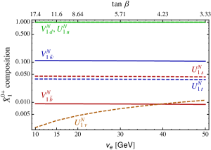
Figure 2: Left panel: $\tilde{\chi}_{4}^{0-}$ (neutrino) and right panel: $\tilde{X}_{1}^{0+}$ (Higgsino-like) composition for $M^{D}_{1}=1$ TeV, $M^{D}_{2}=1.5$ TeV, $\mu=200$ GeV, $\lambda^{S}_{u}=0$ and $\lambda^{T}_{u}=1$, as a function of the sneutrino vev. We plot the absolute magnitude of the rotation matrix elements $V^{N}_{ik}$ and $U^{N}_{ik}$.

Given that both the gluino and wino states are taken to be above a TeV, we shall also take the Dirac bino mass somewhat large, specifically $M^{D}_{1}=1~{}{\rm TeV}$. This is mostly a simplifying assumption, for instance closing squark decay channels into the “second” lightest neutralino (which is bino-like). Thus, the lightest (non SM-like) neutralino is Higgsino-like, and is fairly degenerate with the lightest (non SM-like) chargino, $\tilde{X}^{+-}_{1}$.

In Fig. 2, we show the composition of the physical neutrino ($\tilde{\chi}^{0-}_{4}$) and of the Higgsino-like neutralino state ($\tilde{X}^{0+}_{1}$). Note that, as a result of $R$-charge conservation, the neutrino state has no wino/bino components. In addition, its (up-type) Higgsino component is rather suppressed. As a result, the usual gauge or Yukawa induced interactions are very small. Instead, the dominant couplings of $\tilde{\chi}^{0-}_{4}$ to other states will be those inherited from the neutrino content itself. The associated missing energy signals will then have a character that differs from the one present in mSUGRA-like scenarios. However, it shares similarities with gauge mediation, where the gravitino can play a role similar to the neutrino in our case. By contrast, the “lightest” neutralino, $\tilde{X}^{0+}_{1}$, typically has non-negligible wino/bino components that induce couplings similar to a more standard (massive) neutralino LSP. Nevertheless, here this state decays promptly, and is more profitably thought as a neutralino LSP in the RPV-MSSM (but with 2-body instead of 3-body decays).

2.2 The Scalar Sector

In this section, we discuss the squark, slepton and Higgs sectors, emphasizing the distinctive features compared to other supersymmetric scenarios.

2.2.1 Squarks

Squarks have interesting non-MSSM properties in the present setup. They are charged under the $R$-symmetry ($R=+1$ for the LH squarks and $R=-1$ for the RH ones), and as a result they also carry lepton number. Thus, they are scalar lepto-quarks (strongly interacting particles carrying both baryon and lepton number). This character is given by the superpotential RPV operator $\lambda^{\prime}_{ijk}L_{i}Q_{j}D^{c}_{k}$, which induces decays such as $\tilde{t}_{L}\to b_{R}e^{+}_{L}$. In addition, and unlike in more familiar RPV scenarios, some of these couplings are not free but directly related to Yukawa couplings: $\lambda^{\prime}_{111}=y_{d}$, $\lambda^{\prime}_{122}=y_{s}$ and $\lambda^{\prime}_{133}=y_{b}$. The full set of constraints on the $\lambda^{\prime}$ couplings subject to these relations was analyzed in Ref. [1]. The $\lambda^{\prime}_{333}$ coupling is the least unconstrained, being subject to

$$\lambda^{\prime}_{333} \lesssim (2.1\times 10^{-2})/y_{b}~{}\approx~{}1.4\cos\beta~{},$$ (4)

where $y_{b}=m_{b}/{\textrm{v}}_{\textrm{e}}$, $\tan\beta=v_{u}/{\textrm{v}}_{\textrm{e}}$ and we took $m_{b}(\mu\approx 500~{}{\rm GeV})\approx 2.56~{}{\rm GeV}$ [26]. In this work, we will assume that the only non-vanishing $\lambda^{\prime}$ couplings are those related to the Yukawa couplings, together with $\lambda^{\prime}_{333}$. We will often focus on the case that the upper limit in Eq. (4) is saturated, but should keep in mind that $\lambda^{\prime}_{333}$ could turn out to be smaller, and will comment on the relevant dependence when appropriate.

It is also important to keep in mind that the $R$-symmetry forbids any LR mixing. As a result, the squark eigenstates coincide with the gauge eigenstates, at least if we neglect intergenerational mixing. We will assume in this work that the first two generation squarks are relatively degenerate. As we will see, the current bound on their masses is about $500-700~{}{\rm GeV}$. We will also see that the third generation squarks can be lighter, possibly consistent with estimates based on naturalness from the Higgs sector.

2.2.2 Sleptons

The sleptons are expected to be among the lightest sparticles in the new physics spectrum. This is due to the intimate connection of the slepton sector with EWSB, together with the fact that a good degree of degeneracy between the three generation sleptons is expected. The possible exception is the LH third generation slepton doublet, if the RPV coupling $\lambda^{\prime}_{333}$ turns out to be sizable. As a result, due to RG running, the LH stau can be several tens of GeV lighter than the selectron and smuon, while the latter should have masses within a few GeV of each other. Note that the sleptons are $R$-neutral, hence do not carry lepton number. This is an important distinction compared to the standard extension of lepton number to the new physics sector.

Since the electron sneutrino plays the role of the down-type Higgs, naturalness requires its soft mass to be very close to the electroweak scale. To be definite, we take $m^{2}_{\tilde{L}}\sim m^{2}_{\tilde{E}}\sim($200-300$~{}{\rm GeV})^{2}$. Depending on how this compares to the $\mu$-term, the sleptons can be heavier or lighter than the lightest neutralino, $\tilde{X}^{+-}_{1}$. When $\tilde{X}^{+-}_{1}$ is lighter than the sleptons we will say that we have a “neutralino LSP scenario”. The other case we will consider is one where the LH third generation slepton doublet is lighter than $\tilde{X}^{+-}_{1}$, while the other sleptons are heavier. Given the possible mass gap of several tens of GeV between the $(\tilde{\nu}_{\tau},\tilde{\tau}_{L})$ pair and the other sleptons, this is a rather plausible situation. We will call it the “stau LSP scenario”, although the $\tau$-sneutrino is expected to be up to ten GeV lighter than the stau. The possibility that several or all the sleptons could be lighter than $\tilde{X}^{+-}_{1}$ may also deserve further study, but we will not consider such a case in this work.

We also note that some of the couplings in the RPV operator $\lambda_{ijk}L_{i}L_{j}E^{c}_{k}$ are related to lepton Yukawa couplings: $\lambda_{122}=y_{\mu}$ and $\lambda_{133}=y_{\tau}$. The bounds on the remaining $\lambda_{ijk}$’s under these restriction have been analyzed in [1], and have been found to be stringent. We note that, in principle, it could be possible to produce sleptons singly at the LHC through the $\lambda^{\prime}_{ijk}L_{i}Q_{j}D^{c}_{k}$ operator, with subsequent decays into leptons via the $\lambda_{ijk}L_{i}L_{j}E^{c}_{k}$ induced interactions. We have studied this possibility in Ref [1], and found that there may be interesting signals in the $\mu^{+}\mu^{-}$ and $e^{\mp}\mu^{\pm}$ channels. However, in this work we do not consider such processes any further, and set all $\lambda$ couplings to zero, with the exception of the Yukawa ones. The tau Yukawa, in particular, can play an important role.

2.2.3 The Higgs Sector

The “Higgs” sector is rather rich in our scenario. The EW symmetry is broken by the vev’s of the neutral component of the up-type Higgs doublet, $H^{0}_{u}$, and the electron sneutrino, $\tilde{\nu}_{e}$, which plays a role akin to the neutral down-type Higgs in the MSSM. We have also a scalar SM singlet and a scalar $SU(2)_{L}$ triplet, the superpartners of the singlino and tripletino discussed in the previous section. These scalars also get non-vanishing expectation values. However, it is well known that constraints on the Peskin-Takeuchi $T$-parameter require the triplet vev to be small, $v_{T}\lesssim 2~{}{\rm GeV}$. We will also assume that the singlet vev is in the few GeV range. This means that these two scalars are relatively heavy, and not directly relevant to the phenomenology discussed in this paper. Note that all of these states are $R$-neutral.

There is another doublet, $R_{d}$, the only state with non-trivial $R$-charge ($=+2$). It does not acquire a vev, so that the $R$-symmetry is not spontaneously broken, and therefore this state does not mix with the previous scalars. Its (complex) neutral and charged components are relatively degenerate, with a mass splitting of order 10 GeV, arising from EWSB as well as the singlet vev. For simplicity, we will assume its mass to be sufficiently heavy (few hundred GeV) that it does not play a role in our discussion. Nevertheless, it would be interesting to observe such a state, due to its special $R$-charge.

The upshot is that the light states in the above sector are rather similar to those in the MSSM: a light CP-even Higgs, a heavier CP-even Higgs, a CP-odd Higgs and a charged Higgs pair. The CP-even and CP-odd states are superpositions of the real and imaginary components of $h^{0}_{u}$ and the electron sneutrino (with a small admixture of the singlet and neutral triplet states). Given our choice for the slepton soft masses, the heavy CP-even, CP-odd and charged Higgses are expected to be relatively degenerate, with a mass in the $200-300~{}{\rm GeV}$ range (the charged Higgs being slightly heavier than the neutral states). The charged Higgs is an admixture of $H^{+}_{u}$ and the LH selectron $\tilde{e}_{L}$ (and very suppressed charged tripletino components). The RH selectron, as well as the remaining neutral and charged sleptons do not mix with the Higgs sector, and can be cleanly mapped into the standard slepton/sneutrino terminology.

The light CP-even Higgs, $h$, is special, given the observation of a Higgs-like signal by both the ATLAS [28] and CMS [29] collaborations at about $125~{}{\rm GeV}$. This state can also play an important role in the decay patterns of the various super-particles. Within our scenario, a mass of $m_{h}\approx 125~{}{\rm GeV}$ can be obtained from radiative corrections due to the triplet and singlet scalars, even if both stops are relatively light (recall the suppression of LR mixing due to the $R$-symmetry). This is an interesting distinction from the MSSM. A more detailed study of these issue will be dealt with in a separate paper [30]. Here we point out that these arguments suggest that $\lambda^{S}_{u}$ should be somewhat small, while $\lambda^{T}_{u}$ should be of order one. This motivates our specific benchmark choice: $\lambda^{S}_{u}=0$ and $\lambda^{T}_{u}=1$ (although occasionally we will allow $\lambda^{S}_{u}$ to be non-vanishing). These couplings affect the neutralino/chargino composition and are therefore relevant for the collider phenomenology.

2.3 Summary

Let us summarize the properties of the superpartner spectrum in our scenario, following from the considerations in the previous sections. All the gauginos (“gluino”, “wino” and “bino”) are relatively heavy, in particular heavier than all the sfermions. The first two generation squarks can be below $1~{}{\rm TeV}$, while the third generation squarks can be in the few hundred GeV range. These bounds will be discussed more fully in the remaining of the paper. The sleptons, being intimately connected to the Higgs sector, are in the couple hundred GeV range. So are the “lightest” neutralino and chargino states, which are Higgsino-like. Mixing due to the electron sneutrino vev, induces interesting couplings of the new physics states to the electron-neutrino and the electron, while new interactions related to the lepton and down-quark Yukawa couplings give rise to non-MSSM signals. The collider phenomenology is largely governed by a new (approximately) conserved $R$-charge, and will be seen to be extremely rich, even though the spectrum of light states does not seem, at first sight, very complicated or unconventional. Finally, we mention that there is also an $SU(3)_{C}$ octet scalar (partner of the octetinos that are part of the physical gluino states) that will not be studied here (for studies of the octet scalar phenomenology, see [31, 32]).

3 Sparticle Decay Modes

In this section we discuss the decay modes of the superparticles relevant for the LHC collider phenomenology. We have checked that three-body decays are always negligible and therefore we focus on the two-body decays.

3.1 Neutralino Decays

From our discussion in the previous section, the lightest (non SM-like) neutralino is a Higgsino-like state (that we call $\tilde{X}_{1}^{0+}$), while the truly stable neutralino state is none other than the electron-neutrino. It was also emphasized that $\tilde{X}_{1}^{0+}$ has small, but not always negligible, gaugino components. The other two (Dirac) neutralino states are heavy. We therefore focus here on the decay modes of $\tilde{X}_{1}^{0+}$.

As explained in Subsection 2.2.2, we consider two scenarios: a “neutralino LSP scenario”, where $\tilde{X}_{1}^{0+}$ is lighter than the LH third generation slepton doublet, and a “stau LSP scenario” with the opposite hierarchy. The decay modes of the lightest neutralino depend on this choice and we will consider them separately.

Neutralino LSP Scenario:

If $\tilde{X}_{1}^{0+}$ is lighter than the $(\tilde{\nu}_{\tau},\tilde{\tau}^{-}_{L})$ pair, the possible decay modes for $\tilde{X}_{1}^{0+}$ have partial decay widths [in the notation of Eqs. (1)-(3)]:

$$\Gamma(\tilde{X}^{0+}_{1}\rightarrow W^{-}e^{+}_{L}) = \frac{g^{2}m_{\tilde{X}^{0}_{1}}}{128\pi}\,(U^{+}_{1e}U^{N}_{1\nu}+\sqrt{2}\,U^{+}_{1\tilde{t}}U^{N}_{1\tilde{t}})^{2}\left(1-\frac{M_{W}^{2}}{m_{\tilde{X}^{0}_{1}}^{2}}\right)^{2}\left(2+\frac{m_{\tilde{X}^{0}_{1}}^{2}}{M_{W}^{2}}\right)~{},$$ (5)

$$\Gamma(\tilde{X}^{0+}_{1}\rightarrow Z\bar{\nu}_{e}) = \frac{g^{2}m_{\tilde{X}^{0}_{1}}}{512\pi c_{W}^{2}}(U^{N}_{1\nu}U^{N}_{4\nu}-U^{N}_{1u}U^{N}_{4u})^{2}\left(1-\frac{M_{Z}^{2}}{m_{\tilde{X}^{0}_{1}}^{2}}\right)^{2}\left(2+\frac{m_{\tilde{X}^{0}_{1}}^{2}}{M_{Z}^{2}}\right)~{},$$ (6)

$$\Gamma(\tilde{X}^{0+}_{1}\rightarrow h\bar{\nu}_{e}) = \frac{m_{\tilde{X}^{0}_{1}}}{256\pi}\left(1-\frac{m_{h}^{2}}{m_{\chi^{0}_{1}}^{2}}\right)^{2}\times$$

$$\left[\left(-gV^{N}_{1\tilde{w}}U^{N}_{4u}+g^{\prime}V^{N}_{1\tilde{b}}U^{N}_{4u}\right)R_{1u}+\left(gV^{N}_{1\tilde{w}}U^{N}_{4\nu}-g^{\prime}V^{N}_{1\tilde{b}}U^{N}_{4\nu}\right)R_{1\tilde{\nu}}\right.$$

$$\left.\mbox{}+\sqrt{2}\left(\lambda^{S}_{u}U^{N}_{4\tilde{s}}+\lambda^{T}_{u}U^{N}_{4\tilde{t}}\right)V^{N}_{1d}R_{1u}+\sqrt{2}V^{N}_{1d}U^{N}_{4u}\left(\lambda^{S}_{u}R_{1s}+\lambda^{T}_{u}R_{1t}\right)\right]^{2}~{},$$

where we denote the $\tilde{X}_{1}^{0+}$ mass by $m_{\tilde{X}^{0}_{1}}$, and $R_{1i}$ are the mixing angles characterizing the composition of the lightest Higgs, $h$. In our scenario all the other Higgs bosons are heavier than the lightest neutralino. We note that the above expressions contain an explicit factor of $1/\sqrt{2}$ for each occurrence of a neutralino mixing angle, compared to the standard ones [33, 34, 35]. This is because the mixing matrix elements, $U^{N}_{ij}$ and $V^{N}_{ij}$ are defined in a Dirac basis, whereas in the usual approach the neutralinos are intrinsically Majorana particles. Recall also that, for simplicity, we are assuming here that all quantities are real. The generalization of these and subsequent formulas to the complex case should be straightforward.

Figure 3: $\tilde{X}^{0+}_{1}$ branching fractions in the “neutralino LSP scenario” for $M^{D}_{1}=1$ TeV $M^{D}_{2}=1.5$ TeV, and $\mu=200$ GeV. In the left panel we take $\lambda^{S}_{u}=0$ and $\lambda^{T}_{u}=1$, and in the right panel we take $\lambda^{S}_{u}=\lambda^{T}_{u}=0.4$. The former case might be favored by the observation of a Higgs-like state at $m_{h}\approx 125~{}{\rm GeV}$. We also take the Higgs mixing angles as $R_{1u}\approx 0.98$, $R_{1\tilde{\nu}}\approx 0.2$ and $R_{1s},R_{1t}\ll 1$.

The above decay modes can easily be dominated by the neutrino-neutralino mixing angles, since the contributions due to the higgsino ($U^{N}_{4u}$) and tripletino components are highly suppressed. This mixing angles, in turn, are controlled by the sneutrino vev. Note that in the RPV-MSSM such decay modes are typically characterized by displaced vertices due to the extremely stringent bounds on the sneutrino vev arising from neutrino physics [36]. By contrast, in our scenario the sneutrino vev is allowed to be sizable (tens of GeV), and is in fact bounded from below from perturbativity/EWPT arguments, so that these decays are prompt.

The left panel of Fig. 3 shows that the decay width into $h\bar{\nu}_{e}$ is the dominant one in the small sneutrino vev limit, while in the large sneutrino vev limit the channels involving a gauge boson can be sizable. We also note that it is possible for the $W^{-}e^{+}_{L}$ decay channel to be the dominant one, as shown in the right panel of Fig. 3. In this case we have chosen $\lambda^{S}_{u}=\lambda^{T}_{u}=0.4$, which leads to a cancellation between the mixing angles such that $Z\bar{\nu}_{e}$ is suppressed compared to $W^{-}e^{+}_{L}$. For such small couplings, the radiative contributions to the lightest CP-even Higgs are not large enough to account for the observed $m_{h}\approx 125~{}{\rm GeV}$, while stops (due to the absence of LR mixing) are also not very effective for this purpose. Therefore, without additional physics such a situation may be disfavored. We mention it, since it is tied to a striking signal, which one should nevertheless keep in mind.

Stau LSP Scenario:

If instead the $(\tilde{\nu}_{\tau},\tilde{\tau}^{-}_{L})$ pair is lighter than $\tilde{X}_{1}^{0+}$, the $\tilde{\tau}^{-}_{L}\tau^{+}_{L}$ and $\tilde{\nu}_{\tau}\bar{\nu}_{\tau}$ channels open up with partial decay widths given by

$$\Gamma(\tilde{X}^{0+}_{1}\rightarrow\tilde{\tau}^{-}_{L}\tau^{+}_{L}) \approx \frac{g^{2}}{64\pi}\left(V^{N}_{1\tilde{w}}+\tan{\theta_{W}}V_{1\tilde{b}}^{N}\right)^{2}m_{\tilde{X}^{0}_{1}}\left(1-\frac{m_{\tilde{\tau}_{L}}^{2}}{m_{\tilde{X}^{0}_{1}}^{2}}\right)^{2}~{},$$ (8)

$$\Gamma(\tilde{X}^{0+}_{1}\rightarrow\tilde{\nu}_{\tau}\nu_{\tau}) = \frac{g^{2}}{64\pi}\left(V^{N}_{1\tilde{w}}-\tan{\theta_{W}}V_{1\tilde{b}}^{N}\right)^{2}m_{\tilde{X}^{0}_{1}}\left(1-\frac{m_{\tilde{\nu}_{\tau}}^{2}}{m_{\tilde{X}^{0}_{1}}^{2}}\right)^{2}~{}.$$ (9)

Figure 4: $\tilde{X}^{0+}_{1}$ branching fractions in the “stau LSP scenario” for $M^{D}_{1}=1$ TeV, $M^{D}_{2}=1.5$ TeV, $\mu=250$ GeV, $\lambda^{S}_{u}=0$ and $\lambda^{T}_{u}=1$. We also take $m_{\tilde{\tau}_{L}}\approx~{}m_{\tilde{\nu}_{\tau}}=200~{}{\rm GeV}$. The Higgs mixing angles are as in Fig. 3.

In Eq. (8) we have suppressed additional terms proportional to the $\tau$ Yukawa coupling, that give negligible contributions compared to the ones displayed. Although we have included the full expressions in the numerical analysis, we choose to not display such terms to make the physics more transparent. The only cases where contributions proportional to the Yukawa couplings are not negligible occur when the top Yukawa is involved. We then see that Eqs. (8) and (9) are controlled by the gaugino components, even for the suppressed $V^{N}_{1\tilde{w}}$ and $V^{N}_{1\tilde{b}}$ shown in Fig. 2. Thus, these decay channels dominate over the ones driven by the neutrino-neutralino mixing, as shown in Fig. 4. Here the $\tilde{\nu}_{\tau}\bar{\nu}_{\tau}$ channel is slightly suppressed compared to the one into the charged lepton and slepton due to a cancellation between the mixing angles in Eq. (8). In other regions of parameter space such a cancellation may be more or less severe.

3.2 Chargino Decays

The lightest of the charginos (other than the electron) is $\tilde{X}^{+-}_{1}$. It is Higgsino-like, which follows from its $R=-Q$ nature, and the fact that the winos are heavy. Note that, in contrast, the electron and the other charged leptons have $R=Q$. Therefore, the two-body decays of $\tilde{X}^{+-}_{1}$ can involve a charged lepton only when accompanied with an electrically neutral, $|R|=2$ particle, the only example of which is the $R^{0}_{d}$ scalar. However, this state does not couple directly to the leptons. We take it to be heavier than $\tilde{X}^{+-}_{1}$, which has important consequences for the allowed chargino decay modes. For instance, in the region where $\tilde{\tau}_{L}$ is heavier than $\tilde{X}^{+-}_{1}$ the potentially allowed decay modes of $\tilde{X}^{+-}_{1}$ are into $W^{+}\nu_{e}$ and $W^{+}\tilde{X}^{0-}_{1}$, where $\tilde{X}^{0-}_{1}$ denotes the antiparticle of $\tilde{X}^{0+}_{1}$. However, the second channel is closed in most of the parameter space since $\tilde{X}^{0+}_{1}$ and $\tilde{X}^{+-}_{1}$ are relatively degenerate (with a mass splitting of order ten ${\rm GeV}$). The dominant decay mode in this “neutralino LSP scenario” has a partial decay width given by:

$$\Gamma(\tilde{X}^{+-}_{1}\rightarrow W^{+}\nu_{e}) = \frac{g^{2}}{128\pi}(V^{-}_{1u}U^{N}_{4u}-\sqrt{2}V^{-}_{1\tilde{t}}U^{N}_{4\tilde{t}})^{2}m_{\tilde{X}^{\pm}_{1}}\left(1-\frac{M_{W}^{2}}{m_{\tilde{X}^{\pm}_{1}}^{2}}\right)^{2}\left(2+\frac{m_{\tilde{X}^{\pm}_{1}}^{2}}{M_{W}^{2}}\right)~{},$$ (10)

where we denote the mass of $\tilde{X}^{+-}_{1}$ by $m_{\tilde{X}^{\pm}_{1}}$. Therefore, for sufficiently heavy sleptons the chargino always decays into $W^{+}\nu_{e}.$

If instead $\tilde{\tau}_{L}$ is lighter than $\tilde{X}^{+-}_{1}$ one can also have $\tilde{X}^{+-}_{1}\rightarrow\tilde{\tau}^{+}_{L}\nu_{\tau}$ with

$$\Gamma(\tilde{X}^{+-}_{1}\rightarrow\ \tilde{\tau}^{+}_{L}\nu_{\tau}) = \frac{g^{2}}{32\pi}(U^{-}_{1\tilde{w}})^{2}m_{\tilde{X}^{\pm}_{1}}\left(1-\frac{m_{\tilde{\tau}_{L}}^{2}}{m_{\tilde{X}^{\pm}_{1}}^{2}}\right)^{2}~{}.$$ (11)

Typically, this decay channel dominates, but the $W^{+}\nu_{e}$ can still have an order one branching fraction.

3.3 Slepton Decays

Figure 5: $\tilde{\tau}_{L}$ (solid lines) and $\tilde{\nu}_{\tau}$ (dashed lines) decay modes for two masses: $m_{\tilde{\tau}_{L}}\approx m_{\tilde{\nu}_{\tau}}=180~{}{\rm GeV}$ (left panel) and $m_{\tilde{\tau}_{L}}\approx m_{\tilde{\nu}_{\tau}}=250~{}{\rm GeV}$ (right panel). It is assumed that $\tilde{X}^{0+}_{1}$ is heavier than the $(\tilde{\nu}_{\tau},\tilde{\tau}_{L})$ pair, and that $\lambda^{\prime}_{333}$ saturates Eq. (4).

We focus on the decays of the $(\tilde{\nu}_{\tau},\tilde{\tau}_{L})$ pair since it may very well be the “LSP”, i.e. the last step in a cascade decade to SM particles. In this case the charged slepton decay modes are $\tilde{\tau}^{-}_{L}\to\tau^{-}_{R}\bar{\nu}_{e}$ and $\tilde{\tau}^{-}_{L}\to\bar{t}_{L}b_{R}$, with partial decay widths given by:

$$\Gamma(\tilde{\tau}^{-}_{L}\rightarrow\tau^{-}_{R}\bar{\nu}_{e}) = \frac{m_{\tilde{\tau}_{L}}}{16\pi}\,y_{\tau}^{2}~{},$$ (12)

$$\Gamma(\tilde{\tau}^{-}_{L}\rightarrow\bar{t}_{L}b_{R}) = \frac{m_{\tilde{\tau}_{L}}}{16\pi}\,(\lambda^{\prime}_{333})^{2}\left(1-\frac{m_{t}^{2}}{m_{\tilde{\tau}_{L}^{2}}}\right)^{2}~{}.$$ (13)

The decay widths for the $SU(2)_{L}$ related processes, $\tilde{\nu}_{\tau}\to\tau^{-}_{R}e^{+}_{L}$ and $\tilde{\nu}_{\tau}\to\bar{b}_{L}b_{R}$, are obtained from Eqs. (12) and (13) with the replacements $m_{\tilde{\tau}_{L}}\to m_{\tilde{\nu}_{\tau}}$ and $m_{t}\to m_{b}$. In Fig. 5, we show the branching fractions as a function of the sneutrino vev, assuming that $\lambda^{\prime}_{333}$ saturates Eq. (4), and taking $m_{\tau}=1.7~{}{\rm GeV}$. We see that the $\bar{t}_{L}b_{R}$ channel can be sizable in the large sneutrino vev/small $\tan\beta$ limit, in spite of the phase space suppression when $m_{\tilde{\tau}_{L}}\sim m_{t}+m_{b}$ (left panel). Away from threshold, it can easily dominate (right panel).

If, on the other hand, $\tilde{X}^{0+}_{1}$ and $\tilde{X}^{+-}_{1}$ are lighter than the LH third generation sleptons, their dominant decay modes would be $\tilde{\tau}^{-}_{L}\to\tilde{X}^{0+}_{1}\tau^{-}_{L}$ or $\tilde{\tau}^{+}_{L}\to\tilde{X}^{+-}_{1}\bar{\nu}_{\tau}$, for the charged lepton, and $\tilde{\nu}_{\tau}\to\tilde{X}^{0+}_{1}\nu_{\tau}$ or $\tilde{\nu}_{\tau}\to\tilde{X}^{+-}_{1}\tau^{+}_{L}$ for the sneutrino.

3.4 Squark Decays

As already explained, we focus on the case where the gluinos are heavier than the squarks and, therefore, the squark decay mode into a gluino plus jet is kinematically closed. The lightest neutralinos and charginos are instead expected to be lighter than the squarks since naturalness requires the $\mu$-term to be at the electroweak scale, while we will see that the first and second generation squarks have to be heavier than about $600~{}{\rm GeV}$. Thus, the squark decays into a quark plus the lightest neutralino or into a quark plus the lightest chargino should be kinematically open. However, the decay mode of the left handed up-type squarks, which have $Q=2/3$ and $R=1$, into the lightest chargino $\tilde{X}_{1}^{+-}$ plus a ($R$-neutral) jet is forbidden by the combined conservation of the electric and R-charges: $\tilde{u}_{L}~{}/{\!\!\!\!\to}~{}\tilde{X}_{1}^{+-}j$. The decay mode into the second lightest neutralino, which can be of the $(++)$ type, could be allowed by the quantum numbers, but our choice $M^{D}_{1}>m_{\tilde{q}}$ ensures that it is kinematically closed. Note also that since $u_{R}$ has $Q=2/3$ and $R=-1$, one can have $\tilde{u}_{R}\to\tilde{X}_{1}^{+-}j$.

3.4.1 First and Second Generation Squarks

• The left-handed up-type squarks, $\tilde{u}_{L}$ and $\tilde{c}_{L}$, decay into $\tilde{X}^{0+}_{1}j$ and $e^{+}_{L}j$ with:

  $$\Gamma(\tilde{u}_{L}\rightarrow\tilde{X}^{0+}_{1}j) \approx \frac{m_{\tilde{q}}}{32\pi}\left[\frac{1}{18}\left(g^{\prime}V^{N}_{1\tilde{b}}+3gV^{N}_{1\tilde{w}}\right)^{2}\right]\left(1-\frac{m_{\tilde{X}^{0}_{1}}^{2}}{m_{\tilde{q}}^{2}}\right)^{2}~{},$$ (14)

  $$\Gamma(\tilde{u}_{L}\rightarrow e^{+}_{L}j) = \frac{m_{\tilde{q}}}{16\pi}\,y_{d}^{2}\,(U^{+}_{1e})^{2}~{},$$ (15)

  and analogous expressions for $\tilde{c}_{L}$ (in Eq. (14), we do not display subleading terms proportional to the Yukawa couplings). The second decay is an example of a lepto-quark decay mode. However, taking into account the smallness of the Yukawa couplings for the first two generations, together with the $\tilde{X}_{1}^{0+}$ composition shown in Fig. 2, one finds that the dominant decay mode is the one into neutralino and a jet. Therefore, in the region of parameter space we are interest in, $\tilde{u}_{L}$ and $\tilde{c}_{L}$ decay into $\tilde{X}_{1}^{0+}j$ with almost $100\%$ probability.

• The down-type left-handed squarks, $\tilde{d}_{L}$ and $\tilde{s}_{L}$, have the following decay channels:

  $$\Gamma(\tilde{d}_{L}\rightarrow\tilde{X}_{1}^{0+}j) \approx \frac{m_{\tilde{q}}}{32\pi}\left[\frac{1}{18}\left(g^{\prime}V^{N}_{1\tilde{b}}-3gV^{N}_{1\tilde{w}}\right)^{2}\left(U^{N}_{1\nu}\right)^{2}\right]\left(1-\frac{m_{\tilde{X}^{0}_{1}}^{2}}{m_{\tilde{q}}^{2}}\right)^{2}~{},$$ (16)

  $$\Gamma(\tilde{d}_{L}\rightarrow\tilde{X}^{-+}_{1}j) \approx \frac{m_{\tilde{q}}}{16\pi}\left[g^{2}(U^{-}_{1\tilde{w}})^{2}\right]\left(1-\frac{m_{\tilde{X}^{\pm}_{1}}^{2}}{m_{\tilde{q}}^{2}}\right)^{2}~{},$$ (17)

  $$\Gamma(\tilde{d}_{L}\rightarrow\bar{\nu}_{e}j) = \frac{m_{\tilde{q}}}{32\pi}\,y_{d}^{2}(U^{N}_{4\nu})^{2}~{},$$ (18)

  with analogous expressions for $\tilde{s}_{L}$. The relative minus sign in the gaugino contributions to the neutralino decay channel is due to the $SU(2)$ charge of the down-type squarks, and should be compared to the up-type case, Eq. (14). This leads to a certain degree of cancellation between the contributions from the bino and wino components, which together with the factor of $1/18$ results in a significant suppression of the neutralino channel. Since the Yukawa couplings are very small, it follows that the chargino channel is the dominant decay mode of the down-type squarks of the first two generations.

• The right-handed up-type squarks, $\tilde{u}_{R}$ and $\tilde{c}_{R}$, decay according to

  $$\Gamma(\tilde{u}^{*}_{R}\rightarrow\tilde{X}_{1}^{0+}j) \approx \frac{m_{\tilde{q}}}{32\pi}\,\left[\frac{8}{9}\,(g^{\prime}V^{N}_{1\tilde{b}})^{2}\right]\left(1-\frac{m_{\tilde{X}^{0}_{1}}^{2}}{m_{\tilde{q}}^{2}}\right)^{2}~{},$$ (19)

  $$\Gamma(\tilde{u}_{R}\rightarrow\tilde{X}^{+-}_{1}j) = \frac{m_{\tilde{q}}}{16\pi}\,(y_{u}V^{-}_{1u})^{2}\left(1-\frac{m_{\tilde{X}^{\pm}_{1}}^{2}}{m_{\tilde{q}}^{2}}\right)^{2}~{},$$ (20)

  with analogous expressions for $\tilde{c}_{R}$. The chargino decay mode fo $\tilde{u}_{R}$ is suppressed since the up-type Yukawa coupling is very small. Therefore, the right-handed up-type squark decays into $\tilde{X}^{0+}_{1}j$ with almost $100\%$ probability. However, the charm Yukawa coupling is such that the various terms in Eqs. (19) and (20) are comparable when the mixing angles are as in Figs. 1 and 2. For this benchmark scenario, both decay channels happen to be comparable, as illustrated in the left panel of Fig. 6. Here we used $y_{c}=m_{c}/\sqrt{v^{2}-v^{2}_{e}}$ with $m_{c}(\mu\approx 600~{}{\rm GeV})\approx 550~{}{\rm MeV}$ [26].

  Figure 6: Branching fractions for $\tilde{c}_{R}$ (left panel) and $\tilde{s}_{R}$ (right panel) taking $M^{D}_{1}=1$ TeV, $M^{D}_{2}=1.5$ TeV, $\mu=200$ GeV, $\lambda^{S}_{u}=0$ and $\lambda^{T}_{u}=1$.

• The right-handed down-type squarks, $\tilde{d}_{R}$ and $\tilde{s}_{R}$, decay according to

  $$\Gamma(\tilde{d}^{*}_{R}\rightarrow\tilde{X}_{1}^{0+}j) \approx \frac{m_{\tilde{q}}}{32\pi}\left[\frac{2}{9}\,(g^{\prime}\,V^{N}_{1\tilde{b}})^{2}\right]\left(1-\frac{m_{\tilde{X}^{0}_{1}}^{2}}{m_{\tilde{q}}^{2}}\right)^{2}~{},$$ (21)

  $$\Gamma(\tilde{d}_{R}\rightarrow e^{-}_{L}j) = \frac{m_{\tilde{q}}}{16\pi}\,y_{d}^{2}\,(U^{+}_{1e})^{2}~{},$$ (22)

  $$\Gamma(\tilde{d}_{R}\rightarrow\nu_{e}j) = \frac{m_{\tilde{q}}}{32\pi}\,y_{d}^{2}\,(U^{N}_{4\nu})^{2}~{},$$ (23)

  with analogous expressions for $\tilde{s}_{R}$. Again, for the down squark the Yukawa couplings are negligible so that it decays dominantly into neutralino plus jet. For the strange squark, however, the various channels can be competitive as illustrated in the right panel of Fig. 6. Here we used $y_{s}=m_{s}/{\textrm{v}}_{\textrm{e}}$ with $m_{s}(\mu\approx 600~{}{\rm GeV})\approx 49~{}{\rm MeV}$ [26].

3.4.2 Third Generation Squarks

For the third generation we expect the lepto-quark signals to be visible in all of our parameter space, although they may be of different types. The point is that the bottom Yukawa coupling can be sizable in the small sneutrino vev/large $\tan\beta$ limit (as in the MSSM), thus leading to a signal involving first generation leptons through the $\lambda^{\prime}_{133}\equiv y_{b}\approx 1.15\times 10^{-2}\sec\beta$ coupling. In the large sneutrino vev/small $\tan\beta$ limit, on the other hand, the RPV coupling $\lambda^{\prime}_{333}\lesssim 1.4\cos\beta$ can be of order of $g^{\prime}$, and may lead to third generation leptons in the final state.

Figure 7: Branching fractions for the $\tilde{t}_{L}$ decay modes computed for $M^{D}_{1}=1$ TeV, $M^{D}_{2}=1.5$ TeV, $\mu=200$ GeV, $\lambda^{S}_{u}=0$ and $\lambda^{T}_{u}=1$. We also assume $\lambda_{333}^{\prime}=(2.1\times 10^{-2})/y_{b}$. In the left panel we take $m_{\tilde{t}_{L}}=500~{}{\rm GeV}$, and show the dependence on the sneutrino vev. In the left panel we show the dependence on $m_{\tilde{t}_{L}}$ for ${\textrm{v}}_{\textrm{e}}=10~{}{\rm GeV}$ (solid lines) and ${\textrm{v}}_{\textrm{e}}=50~{}{\rm GeV}$ (dashed lines).

• The left-handed stop, $\tilde{t}_{L}$, has the following decay modes:

  $$\Gamma(\tilde{t}_{L}\rightarrow\tilde{X}_{1}^{0+}t) = \frac{m_{\tilde{t}_{L}}}{32\pi}\left\{\left[\frac{1}{18}\left(g^{\prime}V^{N}_{1\tilde{b}}+3gV^{N}_{1\tilde{w}}\right)^{2}+y_{t}^{2}(U^{N}_{1u})^{2}\right]\left(1-\frac{m^{2}_{\tilde{X}_{1}^{0}}}{m^{2}_{\tilde{t}_{L}}}-\frac{m^{2}_{t}}{m^{2}_{\tilde{t}_{L}}}\right)\right.$$ (24)

  $$\hskip 8.53581pt\left.\mbox{}-\frac{2}{3}\sqrt{2}\,y_{t}U^{N}_{1u}\left(g^{\prime}V^{N}_{1\tilde{b}}+3gV^{N}_{1\tilde{w}}\right)\frac{m_{t}m_{\tilde{X}_{1}^{0}}}{m^{2}_{\tilde{t}_{L}}}\rule{0.0pt}{19.91692pt}\right\}\lambda(m_{\tilde{t}_{L}},m_{\tilde{X}_{1}^{0}},m_{t})~{},$$

  $$\Gamma(\tilde{t}_{L}\rightarrow e^{+}_{L}b_{R}) = \frac{m_{\tilde{t}_{L}}}{16\pi}\,y_{b}^{2}\,(U^{+}_{1e})^{2}~{},$$ (25)

  $$\Gamma(\tilde{t}_{L}\rightarrow\tau^{+}_{L}b_{R}) = \frac{m_{\tilde{t}_{L}}}{16\pi}\,(\lambda_{333}^{\prime})^{2}~{},$$ (26)

  where

  $$\lambda(m_{1},m_{2},m_{3})=\sqrt{1+\frac{m_{2}^{4}}{m_{1}^{4}}+\frac{m_{3}^{4}}{m_{1}^{4}}-2\left(\frac{m_{2}^{2}}{m_{1}^{2}}+\frac{m_{3}^{2}}{m_{1}^{2}}+\frac{m_{2}^{2}m_{3}^{2}}{m_{1}^{4}}\right)}~{}.$$ (27)

  When kinematically allowed, the decay mode into neutralino plus top is the dominant one since it is driven by the top Yukawa coupling, as shown in Fig. 7. However, this figure also shows that the two lepto-quark decay modes can have sizable branching fractions. In particular, at small sneutrino vev the electron-bottom channel is the dominant lepto-quark decay mode (since it is proportional to the bottom Yukawa), while in the large vev limit the third generation lepto-quark channel dominates [we have assumed that $\lambda_{333}^{\prime}$ saturates the upper bound in Eq. (4)]. The existence of lepto-quark channels with a sizable (but somewhat smaller than one) branching fraction is a distinctive feature of our model, as will be discussed in more detail in the following section. We also note that in the case that $\lambda^{\prime}_{333}$ is negligible and does not saturate the bound in Eq. (4), the $\tilde{t}_{L}\rightarrow\tau^{+}_{L}b_{R}$ channel is no longer present, so that the ${\rm BR}(\tilde{t}_{L}\rightarrow e^{+}_{L}b_{R})$ and ${\rm BR}(\tilde{t}_{L}\rightarrow\tilde{X}_{1}^{0+}t)$ increase in the large sneutrino vev limit (but are qualitatively the same as the left panel of Fig. 7).

• The left-handed sbottom, $\tilde{b}_{L}$, has several decay modes as follows:

  $$\Gamma(\tilde{b}_{L}\rightarrow\tilde{X}_{1}^{0+}b) \approx \frac{m_{\tilde{b}_{L}}}{32\pi}\left[\frac{1}{18}\left(g^{\prime}V^{N}_{1\tilde{b}}-3gV^{N}_{1\tilde{w}}\right)^{2}\right]\left(1-\frac{m_{\tilde{X}^{0}_{1}}^{2}}{m_{\tilde{b}_{L}}^{2}}\right)^{2}~{},$$ (28)

  $$\Gamma(\tilde{b}_{L}\rightarrow\tilde{X}^{-+}_{1}t) = \frac{m_{\tilde{b}_{L}}}{16\pi}\left\{\left[g^{2}(U^{-}_{1\tilde{w}})^{2}+y_{t}^{2}(V^{-}_{1u})^{2}\right]\left(1-\frac{m^{2}_{\tilde{X}_{1}^{\pm}}}{m^{2}_{\tilde{b}_{L}}}-\frac{m^{2}_{t}}{m^{2}_{\tilde{b}_{L}}}\right)\right.$$ (29)

  $$\hskip 28.45274pt\left.\mbox{}+4gy_{t}U^{-}_{1\tilde{w}}V^{-}_{1u}\frac{m_{\tilde{X}_{1}^{\pm}}m_{t}}{m^{2}_{\tilde{b}_{L}}}\right\}\lambda(m_{\tilde{b}_{L}},m_{\tilde{X}_{1}^{\pm}},m_{t})~{},$$

  $$\Gamma(\tilde{b}_{L}\rightarrow\bar{\nu}_{e}b_{R}) = \frac{m_{\tilde{b}_{L}}}{32\pi}\,y_{b}^{2}\,(U^{N}_{4\nu})^{2}~{},$$ (30)

  $$\Gamma(\tilde{b}_{L}\rightarrow\bar{\nu}_{\tau}b_{R}) = \frac{m_{\tilde{b}_{L}}}{16\pi}\,(\lambda_{333}^{\prime})^{2}~{}.$$ (31)

  Figure 8: Branching fractions for $\tilde{b}_{L}$ computed for $M^{D}_{1}=1$ TeV, $M^{D}_{2}=1.5$ TeV, $\mu=200$ GeV, $\lambda^{S}_{u}=0$ and $\lambda^{T}_{u}=1$. We also take $\lambda_{333}^{\prime}=(2.1\times 10^{-2})/y_{b}$, and add together the two neutrino channels ($\bar{\nu}_{e}$ and $\bar{\nu}_{\tau}$). In the left panel we take $m_{\tilde{b}_{L}}=500~{}{\rm GeV}$, and show the dependence on the sneutrino vev. In the left panel we show the dependence on $m_{\tilde{b}_{L}}$ for ${\textrm{v}}_{\textrm{e}}=10~{}{\rm GeV}$ (solid lines) and ${\textrm{v}}_{\textrm{e}}=50~{}{\rm GeV}$ (dashed lines).

  When kinematically open, the dominant decay mode is into a chargino plus top since it is controlled by the top Yukawa coupling. The decays into neutrino plus bottom have always a sizable branching fraction, as can be seen in Fig. 8. However, one should note that when $\lambda^{\prime}_{333}$ is negligible, so that the $\tilde{b}_{L}\rightarrow\bar{\nu}_{\tau}b_{R}$ channel is unavailable, the decay involving a neutrino ($\nu_{e}$ only) decreases as the sneutrino vev increases (being of order 0.3% at ${\textrm{v}}_{\textrm{e}}=50~{}{\rm GeV}$). The other two channels adjust accordingly, but do not change qualitatively.

  Figure 9: Branching fractions for $\tilde{t}_{R}$ as a function of $m_{\tilde{t}_{R}}$ (left panel), and for $\tilde{b}_{R}$ as a function of ${\textrm{v}}_{\textrm{e}}$ (right panel) computed for $M^{D}_{1}=1$ TeV, $M^{D}_{2}=1.5$ TeV, $\mu=200$ GeV, $\lambda^{S}_{u}=0$ and $\lambda^{T}_{u}=1$. For $\tilde{b}_{R}$, we take $\lambda_{333}^{\prime}=(2.1\times 10^{-2})/y_{b}$, assume $m_{\tilde{b}_{R}}\gg m_{\tilde{X}^{0}_{1}},m_{t}$, and add together the two neutrino channels ($\bar{\nu}_{e}$ and $\bar{\nu}_{\tau}$).

• For the right-handed stop, $\tilde{t}_{R}$, the decay widths are:

  $$\Gamma(\tilde{t}^{*}_{R}\rightarrow\tilde{X}_{1}^{0+}\bar{t}_{L}) = \frac{m_{\tilde{t}_{R}}}{32\pi}\left\{\left[\frac{8}{9}\left(g^{\prime}V^{N}_{1\tilde{b}}\right)^{2}+y_{t}^{2}(V^{-}_{1u})^{2}\right]\left(1-\frac{m^{2}_{\tilde{X}_{1}^{0}}}{m^{2}_{\tilde{t}_{L}}}-\frac{m^{2}_{t}}{m^{2}_{\tilde{t}_{L}}}\right)\right.$$ (32)

  $$\hskip 28.45274pt\left.\mbox{}+\frac{8}{3}\sqrt{2}\,y_{t}g^{\prime}V^{N}_{1\tilde{b}}U^{N}_{1u}\frac{m_{t}m_{\tilde{X}_{1}^{0}}}{m^{2}_{\tilde{t}_{L}}}\rule{0.0pt}{19.91692pt}\right\}\lambda(m_{\tilde{t}_{R}},m_{\tilde{X}_{1}^{0}},m_{t})~{},$$

  $$\Gamma(\tilde{t}_{R}\rightarrow\tilde{X}^{+-}_{1}b_{R}) = \frac{m_{\tilde{t}_{R}}}{16\pi}\left(y_{t}V^{-}_{1u}\right)^{2}\left(1-\frac{m_{\tilde{X}_{1}^{0}}^{2}}{m_{\tilde{t}_{R}}^{2}}\right)^{2}~{}.$$ (33)

  For the benchmark choice of $M^{D}_{2}=1.5$ TeV, $M^{D}_{1}=1$ TeV, $\mu=200$ GeV, $\lambda^{S}_{u}=0$ and $\lambda^{T}_{u}=1$, we have $\Gamma(\tilde{t}^{*}_{R}\rightarrow\tilde{X}_{1}^{0+}t_{L})=26\%~{}(15\%)$ and $\Gamma(\tilde{t}_{R}\rightarrow\tilde{X}^{+-}_{1}b_{R})=74\%~{}(85\%)$ for $m_{\tilde{t}_{R}}=500~{}(400)~{}{\rm GeV}$, independently of the sneutrino vev. For $m_{\tilde{t}_{R}}<m_{\tilde{X}^{0}_{1}}+m_{t}$, the RH stop decays into $\tilde{X}^{+-}_{1}b_{R}$ essentially 100% of the time. See left panel of Fig. 9.

• The right-handed sbottom, $\tilde{b}_{R}$, has a variety of decay modes:

  $$\Gamma(\tilde{b}^{*}_{R}\rightarrow\tilde{X}_{1}^{0+}\bar{b}_{R}) \approx \frac{m_{\tilde{b}_{R}}}{32\pi}\left[\frac{2}{9}\left(g^{\prime}V^{N}_{1\tilde{b}}\right)^{2}\right]\left(1-\frac{m_{\tilde{X}_{1}^{0}}^{2}}{m_{\tilde{b}_{R}}^{2}}\right)^{2}~{},$$ (34)

  $$\Gamma(\tilde{b}_{R}\rightarrow e^{-}_{L}t_{L}) = \frac{m_{\tilde{b}_{R}}}{16\pi}\,y_{b}^{2}\,(U^{+}_{1e})^{2}\left(1-\frac{m_{t}^{2}}{m_{\tilde{b}_{R}}^{2}}\right)^{2}~{},$$ (35)

  $$\Gamma(\tilde{b}_{R}\rightarrow\nu_{e}b_{L}) = \frac{m_{\tilde{b}_{R}}}{32\pi}\,y_{b}^{2}\,(U^{N}_{4\nu})^{2}~{},$$ (36)

  $$\Gamma(\tilde{b}_{R}\rightarrow\tau^{-}_{L}t_{L}) = \frac{m_{\tilde{b}_{R}}}{16\pi}\,(\lambda_{333}^{\prime})^{2}\left(1-\frac{m_{t}^{2}}{m_{\tilde{b}_{R}}^{2}}\right)^{2}~{},$$ (37)

  $$\Gamma(\tilde{b}_{R}\rightarrow\nu_{\tau}b_{L}) = \frac{m_{\tilde{b}_{R}}}{16\pi}\,(\lambda_{333}^{\prime})^{2}~{}.$$ (38)

  The lepto-quark signals are the dominant ones. Adding the two neutrino channels, the decay mode into $\nu b$ has a branching fraction of about $50\%$ as shown in the right panel of Fig. 9. The charged lepton signals can involve a LH electron or a $\tau$ plus a top quark. Note also that the decay mode into $\tilde{X}_{1}^{0+}b$ is very suppressed. We finally comment on the modifications when $\lambda^{\prime}_{333}$ is negligible. Once the $\tilde{b}_{R}\rightarrow\tau^{-}_{L}t_{L}$ and $\tilde{b}_{R}\rightarrow\nu_{\tau}b_{L}$ channels become unavailable, one has that ${\rm BR}(\tilde{b}_{R}\rightarrow e^{-}_{L}t_{L})\approx 0.6$ and ${\rm BR}(\tilde{b}_{R}\rightarrow\nu_{e}b_{L})\approx 0.4$, independent of the sneutrino vev. The $\tilde{b}^{*}_{R}\rightarrow\tilde{X}_{1}^{0+}\bar{b}_{R}$ channel remains negligible.

4 $1^{\rm st}$ and $2^{\rm nd}$ Generation Squark Phenomenology

In the present section we discuss the LHC phenomenology of the first and second generation squarks, which are expected to be the most copiously produced new physics particles. Although these squarks are not required by naturalness to be light, flavor considerations may suggest that they should not be much heavier than the third generation squarks. Therefore, it is interesting to understand how light these particles could be in our scenario. As we will see, current bounds allow them to be as light as $500-700~{}{\rm GeV}$, while in the MSSM the LHC bounds have already exceeded the $1~{}{\rm TeV}$ threshold. The bounds can arise from generic jets + $\cancel{E}_{T}$ searches, as well as from searches involving leptons in the final state.

4.1 Squark Production

We compute the cross section to produce a given final state $X$ in our model as follows:

$$\sigma(pp\to X) = \sum_{i}\sigma(pp\to i)\times\textrm{BR}(i\to X)~{},$$ (39)

where $i=\tilde{q}_{1}\tilde{q}_{2},\tilde{g}\tilde{q},\tilde{g}\tilde{g}$, and the squark pair production can in principle come in several flavor and chirality combinations. We generate the production cross section for each independent $i$-th state with MadGraph5 [37]. Here we note that, due to the assumption of gluinos in the multi-TeV range, and the fact that we will be interested in squarks below 1 TeV, our cross section is dominated by the production of squark pairs. We have also computed the corresponding $K$-factor with Prospino2 [25], as a function of the squark mass for fixed (Majorana) gluino masses of $2-5$ TeV. We find that for squark masses below about 1 TeV, the K-factor is approximately constant with $K\approx 1.6$. Since, to our knowledge, a NLO computation in the Dirac case is not available, we will use the previous K-factor to obtain a reasonable estimate of the Dirac NLO squark pair-production cross-section.

Figure 10: Left Panel: $\tilde{q}\tilde{q}^{*}$ production cross-section (all flavor combinations), for the 7 TeV LHC run, computed for 2 TeV Dirac (red) and Majorana (blue) gluinos. In the right panel we plot the ratio between the two cross sections, showing that the suppression in the Dirac case can be significant.

One should note that the Dirac nature of the gluinos results in a significant suppression of certain $t$-channel mediated gluino diagrams compared to the Majorana (MSSM) case, as already emphasized in [14, 15] (see also Fig. 10). Nevertheless, at $M_{\tilde{g}}=2$ TeV such contributions are not always negligible, and should be included. For instance, we find that for degenerate squark with $m_{\tilde{q}}=800~{}{\rm GeV}$, the production of $\tilde{u}_{L}\tilde{u}_{R}$, $\tilde{u}_{L}\tilde{d}_{R}$ and $\tilde{u}_{R}\tilde{d}_{L}$ is comparable to the “diagonal” production of $\tilde{q}_{L}\tilde{q}^{*}_{L}$ and $\tilde{q}_{R}\tilde{q}^{*}_{R}$ for all the squark flavors $\tilde{q}=\tilde{u},\tilde{d},\tilde{s},\tilde{c}$ taken together. As indicated in Eq. (39) we include separately the BR for each $i$-th state to produce the final state $X$, since these can depend on the squark flavor, chirality or generation.

4.2 “Simplified Model” Philosophy

We have seen that $\tilde{u}_{L}$, $\tilde{u}_{R}$, $\tilde{d}_{R}$ and $\tilde{c}_{L}$ decay dominantly through the neutralino channel, the LH down-type squarks, $\tilde{d}_{L}$ and $\tilde{s}_{L}$, decay dominantly through the chargino channel, and $\tilde{c}_{R}$ and $\tilde{s}_{R}$ can have more complicated decay patterns (see Fig. 6). The striking lepto-quark decay mode, $\tilde{s}_{R}\to e^{-}_{L}j$, will be treated separately. In this section we focus on the decays involving neutralinos and charginos. Since the signals depend on how the neutralino/chargino decays, it is useful to present first an analysis based on the simplified model (SMS) philosophy. To be more precise, we set bounds assuming that the neutralinos/charginos produced in squark decays have a single decay mode with ${\rm BR}=1$. We also separate the “neutralino LSP scenario”, in which $\tilde{X}^{0+}_{1}/\tilde{X}^{+-}_{1}$ decay into SM particles, from the “stau LSP scenario”, where they decay into $\tilde{\tau}^{-}_{L}\tau^{+}_{L}$, $\tilde{\nu}_{\tau}\bar{\nu}_{\tau}$ or $\tilde{\tau}^{+}_{L}\nu_{\tau}$. We will give further details on these subsequent decays below, where we treat the two cases separately.

Figure 11: Cross-sections for the separate production of $\tilde{X}^{0+}_{1}\tilde{X}^{0-}_{1}$, $\tilde{X}^{+-}_{1}\tilde{X}^{-+}_{1}$ and $\tilde{X}^{0+}_{1}\tilde{X}^{+-}_{1}$ trough squark pair-production in the SMS approach (see main text). The solid and dotted lines correspond to $\sigma_{1}$, according to the case. The dashed line marked as $\sigma_{2}$ corresponds to the full pair-production of squarks, irrespective of how they decay. The cross-sections are computed for $M_{\tilde{g}}=2$ TeV for a 7 TeV LHC run, with a K-factor, $K=1.6$.

Here we emphasize that we regard the jets plus $\tilde{X}^{0+}_{1}/\tilde{X}^{+-}_{1}$ stage as part of the production. The point is that an important characteristic of our scenario is that different types of squarks produce overwhelmingly only one of these two states. For instance, if we are interested in two charginos in the squark cascade decays, this means that they must have been produced through LH down-type squarks (with a smaller contribution from $\tilde{c}_{R}\tilde{c}_{R}^{*}$ production), and the production of any of the other squarks would not be relevant to this topology. Conversely, if we are interested in a topology with two neutralinos, the LH down-type squarks do not contribute. We denote by $\sigma_{1}$ the corresponding cross sections, computed via Eq. (39) with $X=``\tilde{X}^{+-}_{1}\tilde{X}^{-+}_{1}jj"$ or $X=``\tilde{X}^{0+}_{1}\tilde{X}^{0-}_{1}jj"$, taking the ${\rm BR}$’s as exactly zero or one, according to the type of squark pair $i$. At the same time, since in other realizations of the $R$-symmetry these production patterns may not be as clear-cut, we will also quote bounds based on a second production cross section, denoted by $\sigma_{2}$, where it is assumed that all the squarks decay either into the lightest neutralino or chargino channels with unit probability. This second treatment is closer to the pure SMS philosophy, but could be misleading in the case that lepton number is an $R$-symmetry. We show the corresponding cross-sections in Fig. 11.

It should also be noted that the great majority of simplified models studied by ATLAS and CMS consider either $m_{\tilde{q}}=M_{\tilde{g}}$, or $m_{\tilde{q}}\gg M_{\tilde{g}}$. Therefore, at the moment there are only a handful of dedicated studies of our topologies, although we will adapt studies performed for other scenarios to our case. In the most constraining cases, we will estimate the acceptance by simulating the signal in our scenario and applying the experimental cuts, but for the most part a proper mapping of the kinematic variables should suffice (provided the topologies are sufficiently similar). A typical SMS analysis yields colored-coded plots for the upper bound on $\sigma\times{\rm BR}$ (or $A\times\epsilon$) for the given process, in the plane of the produced (strongly-interacting) particle mass (call it $m_{\tilde{q}}$), and the LSP mass (call it $m_{\rm LSP}$). In most cases, the LSP is assumed to carry $\cancel{E}_{T}$. Often, there is one intermediate particle in the decay chain. Its mass is parametrized in terms of a variable $x$ defined by $m_{\rm intermediate}=xm_{\tilde{q}}+(1-x)m_{\rm LSP}$. In our “neutralino LSP scenario”, the intermediate particle is either the lightest neutralino $\tilde{X}^{0+}_{1}$ or the lightest chargino $\tilde{X}_{1}^{+-}$, whose masses are set by the $\mu$-term. Since the particle carrying the $\cancel{E}_{T}$ is the neutrino, i.e. $m_{\rm LSP}=0$, we have $x\approx\mu/m_{\tilde{q}}$.

We will set our bounds as follows: we compute our theoretical cross section as described above (i.e. based on the $\sigma_{1}$ or $\sigma_{2}$ production cross-sections) as a function of the squark mass, and considering the appropriate decay channel for the $X^{0+}_{1}/X^{+-}_{1}$ (with ${\rm BR}=1$ in the SMS approach). Provided the topology is sufficiently similar, we identify the $x$-axis on the color-coded plots in the experimental analyses (usually $m_{\tilde{g}}$) with $m_{\tilde{q}}$, take $m_{LSP}=0$ (for the neutrino), and identify “$x$” as $\mu/m_{\tilde{q}}$ (from our discussion above). Then, we increase the squark mass until the theoretical cross-section matches the experimental upper bound, defining a lower bound on $m_{\tilde{q}}$. In a few cases that have the potential of setting strong bounds, but where the experimentally analyzed topologies do not exactly match the one in our model, we obtain the signal $\epsilon\times A$ from our own simulation and use the 95% C.L. upper bound on $\sigma\times\epsilon\times A$ to obtain an upper bound on $\sigma$ that can be compared to our model cross-section. If there are several signal regions, we use the most constraining one.

4.3 Neutralino LSP Scenario

In the neutralino LSP scenario, and depending on the region of parameter space (e.g. the sneutrino vev or the values of the $\lambda_{S}$ and $\lambda_{T}$ couplings), the lightest neutralino, $\tilde{X}_{1}^{0+}$, can dominantly decay into $Z\bar{\nu}_{e}$, $h\bar{\nu}_{e}$ or $W^{-}e^{+}_{L}$. The “lightest” chargino $\tilde{X}_{1}^{+-}$ always decays into $W^{+}\nu_{e}$. Following the philosophy explained in the previous subsection, we set separate bounds on four simplified model scenarios:

• $\tilde{q}\to\tilde{X}_{1}^{0+}j\to(Z\bar{\nu}_{e})\,j$ ,

• $\tilde{q}\to\tilde{X}_{1}^{0+}j\to(h\bar{\nu}_{e})\,j$ ,

• $\tilde{q}\to\tilde{X}_{1}^{0+}j\to(W^{-}e^{-}_{L})\,j$ ,

• $\tilde{q}\to\tilde{X}_{1}^{+-}j\to(W^{+}\nu_{e})\,j$ ,

as well as on two benchmark scenarios (to be discussed in Subsection 4.3.1) that illustrate the bounds on the full model.

Topology	$\sigma_{1}$-bound	$\sigma_{2}$-bound	Search	Reference
	$m_{\tilde{q}}$ [GeV]	$m_{\tilde{q}}$ [GeV]
$\tilde{q}\to\tilde{X}_{1}^{0+}j\to(Z\bar{\nu}_{e})\,j$	640	690	$Z(ll)$ + jets + $\cancel{E}_{T}$	CMS [40]
	635	685	jets + $\cancel{E}_{T}$	ATLAS [19]
$\tilde{q}\to\tilde{X}_{1}^{0+}j\to(h\bar{\nu}_{e})\,j$	605	655	jets + $\cancel{E}_{T}$	ATLAS [19]
$\tilde{q}\to\tilde{X}_{1}^{0+}j\to(W^{-}e^{-}_{L})\,j$	580	630	Multilepton	ATLAS [41]
$\tilde{q}\to\tilde{X}_{1}^{+-}j\to(W^{+}\nu_{e})\,j$	530	650	jets + $\cancel{E}_{T}$	ATLAS [19]
	410	500	Multilepton	ATLAS [42]
	350	430	$l$ + jets + $\cancel{E}_{T}$	ATLAS [43]
Benchmark 1	$590-650$	—	jets + $\cancel{E}_{T}$	ATLAS [19]
Benchmark 2	$520-560$	—	jets + $\cancel{E}_{T}$	ATLAS [19]

Table 1: Bounds on $1^{\rm st}$ and $2^{\rm nd}$ generation squark masses from squark pair production in the “neutralino LSP scenario” for the Simplified Models $(1)$–$(4)$, and two benchmark scenarios. See text for further details.

There are several existing searches that can potentially constrain the model:

• jets + $\cancel{E}_{T}$ ,

• 1 lepton + jets + $\cancel{E}_{T}$ ,

• $Z(ll)$ + jets + $\cancel{E}_{T}$ ,

• OS dileptons + $\cancel{E}_{T}$ + jets ,

• multilepton + jets + $\cancel{E}_{T}$ (with or without Z veto).

We postpone the detailed description of how we obtain the corresponding bounds to the appendix, and comment here only on the results and salient features. We find that typically the most constraining searches are the generic jets + $\cancel{E}_{T}$ searches, in particular the most recent ATLAS search with $5.8~{}{\rm fb}^{-1}$ [19]. In addition, some of the simplified topologies can also be constrained by searches involving leptons + jets + $\cancel{E}_{T}$. For example, those involving a leptonically decaying $Z$ are important for the $\tilde{X}_{1}^{0+}\rightarrow Z\bar{\nu}_{e}$ case, while a number of multi-lepton searches can be relevant for the topologies that involve a $W$. We summarize our findings in Table 1, where we exhibit the searches that have some sensitivity for the given SMS topology. We show the lower bounds on the squark masses based on both the $\sigma_{1}$ and $\sigma_{2}$ production cross-sections, as described in Subsection 4.2. We see that these are below $650$ GeV (based on $\sigma_{1}$; the bound from $\sigma_{2}$ is provided only for possible application to other models). We also show the bounds for two benchmark scenarios (which depend on the sneutrino vev), as will be discussed in the next subsection. These are shown under the $\sigma_{1}$ column, but should be understood to include the details of the branching fractions and various contributing processes. We have obtained the above results by implementing the experimental analysis and computing the relevant $\epsilon\times A$ from our own simulation of the signal, and using the model-independent 95% CL upper bounds on $\sigma\times\epsilon\times A$ provided by the experimental analysis. Whenever possible, we have also checked against similar simplified model interpretations provided by the experimental collaborations. Such details are described in the appendix, where we also discuss other searches that turn out to not be sensitive enough, and the reasons for such an outcome. In many cases, it should be possible to optimize the set of cuts (within the existing strategies) to attain some sensitivity. This might be interesting, for example, in the cases involving a Higgs, given that one might attempt to reconstruct the Higgs mass.

We turn next to the analysis of the full model in the context of two benchmark scenarios.

4.3.1 Realistic Benchmark Points

Figure 12: Cross-sections for a variety of signatures in the “neutralino LSP scenario”. All are computed for $M^{D}_{1}=1$ TeV, $M^{D}_{2}=1.5$ TeV, $\mu=200$ GeV, and assuming that $\lambda^{\prime}_{333}$ saturates Eq. (4). In the left panel we take $m_{\tilde{q}}=700~{}{\rm GeV}$ and $\lambda^{S}_{u}=0$, $\lambda^{T}_{u}=1$ (benchmark 1), while in the right panel we use $m_{\tilde{q}}=550~{}{\rm GeV}$ and $\lambda^{S}_{u}=\lambda^{T}_{u}=0.4$ (benchmark 2).

Besides the “simplified model” type of bounds discussed above, it is also interesting to present the bounds within benchmark scenarios that reflect the expected branching fractions for the neutralinos/charginos discussed in Subsections 3.1 and 3.2. One difference with the analysis of the previous subsections is that we can have all the combinations of $\tilde{X}^{0+}_{1}\tilde{X}_{1}^{0-}jj$, $\tilde{X}^{+-}_{1}\tilde{X}_{1}^{-+}jj$ and $\tilde{X}_{1}^{0+}\tilde{X}^{+-}_{1}jj$ in squark decays, with the corresponding BR’s. In Fig. 11 we have shown the individual cross-sections in the SMS approach. These give a sense of the relative contributions of the various channels. In particular, we see that the $\tilde{X}^{0+}_{1}\tilde{X}_{1}^{0-}$ channel dominates.

Benchmark 1: ($M^{D}_{1}=1$ TeV $M^{D}_{2}=1.5$ TeV, $\mu=200$ GeV, $\lambda^{S}_{u}=0$, $\lambda^{T}_{u}=1$) corresponds to the case that the $\tilde{X}^{0+}_{1}\to h\bar{\nu}_{e}$ decay channel is important (in fact, dominant at small sneutrino vev), while the gauge decay channels of the $\tilde{X}^{0+}_{1}$ can be sizable (see left panel of Fig. 3). The LHC searches relevant to this scenario are:

• jets + $\cancel{E}_{T}$ ,

• 1 lepton + jets + $\cancel{E}_{T}$ ,

• OS dileptons + $\cancel{E}_{T}$ + jets ,

• dileptons (from $Z$ decay) + jets + $\cancel{E}_{T}$ ,

• multilepton + jets + $\cancel{E}_{T}$ (without Z cut).

We apply the model-independent bounds discussed in the previous sections, and find that the jets + $\cancel{E}_{T}$ search is the most constraining one. Using $\sigma_{j+\cancel{E}_{T}}\lesssim 20-40$ fb, we find $m_{\tilde{q}}\gtrsim 620-690~{}{\rm GeV}$ ($m_{\tilde{q}}\gtrsim 590-650~{}{\rm GeV}$) for ${\textrm{v}}_{\textrm{e}}=10~{}{\rm GeV}$ (${\textrm{v}}_{\textrm{e}}=50~{}{\rm GeV}$). We show in the left panel of Fig. 12 the cross-sections for several processes, for $m_{\tilde{q}}=700~{}{\rm GeV}$. These are computed from Eq. (39) using the actual BR’s for the chosen benchmark. Although there is some dependence on the sneutrino vev, the global picture is robust against ${\textrm{v}}_{\textrm{e}}$.

Benchmark 2: ($M^{D}_{1}=1$ TeV, $M^{D}_{2}=1.5$ TeV, $\mu=200$ GeV, $\lambda^{S}_{u}=\lambda^{T}_{u}=0.4$) corresponds to the case that the $\tilde{X}_{1}^{0+}\to W^{-}e^{+}$ decay channel dominates (see right panel of Fig. 3). In the right panel of Fig. 12, we show the cross-sections for the main processes. We see that, for this benchmark, the “leptonic channels” have the largest cross sections (especially the multilepton + jets + $\cancel{E}_{T}$ one). However, taking into account efficiencies of at most a few percent for the leptonic searches (as we have illustrated in the previous section), we conclude that the strongest bound on the squark masses arises instead from the jets + $\cancel{E}_{T}$ searches (as for benchmark 1). Using $\sigma_{j+\cancel{E}_{T}}\lesssim 20-40$ fb, we find $m_{\tilde{q}}\gtrsim 520-580~{}{\rm GeV}$ ($m_{\tilde{q}}\gtrsim 500-560~{}{\rm GeV}$) for ${\textrm{v}}_{\textrm{e}}=10~{}{\rm GeV}$ (${\textrm{v}}_{\textrm{e}}=50~{}{\rm GeV}$). Note that there is a sizable “no missing energy” cross section. However, this could be significantly lower once appropriate trigger requirements are imposed.

4.4 Stau LSP Scenario

In this scenario the dominant decay modes of $\tilde{X}_{1}^{0+}$ are into $\tilde{\tau}^{-}_{L}\tau^{+}_{L}$ or $\tilde{\nu}_{\tau}\bar{\nu}_{\tau}$ (about 50-50), while the chargino $\tilde{X}_{1}^{+-}$ decays into $\tilde{\tau}^{+}_{L}\nu_{\tau}.$ The decay modes of $\tilde{\tau}^{-}_{L}$ depend on the sneutrino vev: for large ${\textrm{v}}_{\textrm{e}}$ it decays dominantly into $\bar{t}_{L}b_{R}$ (assuming $\lambda^{\prime}_{333}$ is sizable), while for smaller values of ${\textrm{v}}_{\textrm{e}}$ it decays dominantly into $\tau^{-}_{R}\bar{\nu}_{e}$ trough the $\tau$ Yukawa coupling. Similarly, $\tilde{\nu}_{\tau}$ decays into $\bar{b}_{L}b_{R}$ for large sneutrino vev, and into $\tau^{-}_{R}e^{+}_{L}$ for small sneutrino vev. In the “stau LSP scenario” we prefer to discuss the two limiting cases of small and large sneutrino vev, rather than present SMS bounds (recall from Fig. 11 that the squarks produce dominantly $\tilde{X}^{0+}_{1}\tilde{X}^{0-}_{1}$ pairs). This scenario is, therefore, characterized by third generation signals.

4.4.1 $\tilde{\tau}^{-}_{L}\rightarrow\tau^{-}_{R}\bar{\nu}_{e}$ and $\tilde{\nu}_{\tau}\to\tau^{-}_{R}e^{+}_{L}$ decay modes

These decays are characteristic of the small sneutrino vev limit. In this case all the final states would contain at least two taus: $i)$ for the $\tilde{X}_{1}^{0+}\tilde{X}_{1}^{0-}$ topology the final state contains 2 jets, missing energy and $2\tau+2e$, $3\tau+1e$ or $4\tau$’s; $ii)$ for the $\tilde{X}_{1}^{0+}\tilde{X}_{1}^{+-}$ topology the final state contains 2 jets, missing energy and $2\tau+1e$ or $3\tau$’s; $iii)$ for the $\tilde{X}_{1}^{-+}\tilde{X}_{1}^{+-}$ topology the final state contains 2 jets, missing energy and $2\tau$’s. It is important that cases $i)$ and $ii)$ can be accompanied by one or two electrons, given that many searches for topologies involving $\tau$’s  impose a lepton ($e$ or $\mu$) veto.

Thus, for instance, a recent ATLAS study [44] with 4.7 fb^-1 searches for jets + $\cancel{E}_{T}$ accompanied by exactly one (hadronically decaying) $\tau$ + one lepton ($e$ or $\mu$), or by two $\tau$’s with a lepton veto. Only the former would apply to our scenario, setting a bound of $\sigma\times\epsilon\times A=0.68~{}{\rm fb}^{-1}$. A previous ATLAS search [45] with 2.05 fb^-1 searches for at least $2\tau$’s (with a lepton veto), setting a bound of $\sigma\times\epsilon\times A=2.9~{}{\rm fb}^{-1}$. However, the efficiency of such searches is lower than the one for jets plus missing energy (also with lepton veto). Since in our scenario the cross sections for these two signatures is the same, the latter will set the relevant current bound.

There is also a CMS study [46] sensitive to $4\tau$ signals in the context of GMSB scenarios, which has a similar topology to our case (SMS: $\tilde{g}\tilde{g}$ production with $\tilde{g}\rightarrow qq\chi^{0}_{1}$ and $\chi^{0}_{1}\to\tau^{+}\tau^{-}\tilde{G}_{\mu}$). From their Fig. 9b, we can see that the 95% CL upper limit on the model cross section varies between $0.3-0.03~{}{\rm pb}$ for $400~{}{\rm GeV}<m_{\tilde{g}}<700~{}{\rm GeV}$. Including the branching fractions, and reinterpreting the bound in the squark mass plane, we find a bound of $m_{\tilde{q}}\gtrsim 600~{}{\rm GeV}$ at ${\textrm{v}}_{\textrm{e}}=10$, where the cross section is about 45 fb. When the sneutrino vev increases the bound gets relaxed so that for ${\textrm{v}}_{\textrm{e}}\gtrsim 20~{}{\rm GeV}$ there is no bound from this study.

The generic searches discussed in previous sections (not necessarily designed for sensitivity to the third generation) may also be relevant:

• jets + $\cancel{E}_{T}$ ,

• jets + $\cancel{E}_{T}$ + 1 lepton ,

• jets + $\cancel{E}_{T}$ + SS dileptons ,

• jets + $\cancel{E}_{T}$ + OS dileptons ,

• jets + $\cancel{E}_{T}$ + multi leptons ,

where the leptons may arise from the $\tilde{\nu}_{\tau}$ decay as in cases $i)$ and $ii)$ above, or from leptonically decaying $\tau$’s. It turns out that, as in the “neutralino LSP scenario”, the strongest bound arises from the jets + $\cancel{E}_{T}$ search. We find from simulation of the signal efficiency times acceptance for the ATLAS analysis [19] in our model that the most stringent bound arises from signal region C (tight), and gives an upper bound on the model cross section of about 120 fb. Thus, we find that $m_{\tilde{q}}\gtrsim 500~{}{\rm GeV}$ for ${\textrm{v}}_{\textrm{e}}=10~{}{\rm GeV}$.

4.4.2 $\tilde{\tau}^{-}_{L}\rightarrow\bar{t}_{L}b_{R}$ and $\tilde{\nu}_{\tau}\to\bar{b}_{L}b_{R}$ decay modes

When the third generation sleptons decay through these channels, as is typical of the large sneutrino vev limit, the signals contain a $b\bar{b}$ and/or a $t\bar{t}$ pair, as well as $\tau$’s. Note that when the $\tau$’s and tops decay hadronically one has a signal without missing energy. However, the branching fraction for such a process is of order ${\rm BR}(\tilde{q}\to\tilde{X}^{0+}_{1}j)^{2}\times{\rm BR}(\tilde{X}^{0+}_{1}\to\tilde{\tau}_{L}^{-}\tau^{+}_{L})^{2}\times{\rm BR}(\tilde{\tau}_{L}^{-}\to\bar{t}_{L}b_{R})^{2}\times{\rm BR}(t\to bW^{+})^{2}\times{\rm BR}(W\to jj)^{2}\times{\rm BR}(\tau\to jj)^{2}\sim$ few per cent (in the large sneutrino vev limit, where all of these branching fractions are sizable). Indeed, we find that the “no $\cancel{E}_{T}$” cross section for $700~{}{\rm GeV}$ squarks in the “stau LSP scenario” is of order $1~{}{\rm fb}$, which is relatively small. Rather, the bulk of the cross section shows in the jets + $\cancel{E}_{T}$ and 1 lepton + jets + $\cancel{E}_{T}$ channels (with a smaller 2 lepton + jets + $\cancel{E}_{T}$ contribution). Simulation of the ATLAS j+$\cancel{E}_{T}$ search [19] in this region of our model indicates that again the most stringent bound arises from signal region C (tight) of this study, and gives an upper bound on the model cross section of about 70 fb. This translates into a bound of $m_{\tilde{q}}\gtrsim 550~{}{\rm GeV}$ for ${\textrm{v}}_{\textrm{e}}=50~{}{\rm GeV}$.

5 Third Generation Squark Phenomenology

We turn now to the LHC phenomenology of the third generation squarks. We start by studying the current constraints and then we will explain how the third generation provides a possible smoking gun for our model. We separate our discussion into the signals arising from the lepto-quark decay channels, and those that arise from the decays of the third generation squarks into states containing $\tilde{X}^{0+}_{1}$ or $\tilde{X}^{+-}_{1}$ (or their antiparticles).

5.1 Lepto-quark Signatures

Due to the identification of lepton number as an $R$-symmetry, there exist lepto-quark (LQ) decays proceeding through the $LQD^{c}$ couplings. These can be especially significant for the third generation squarks. As discussed in Subsection 3.4.2, in our scenario we expect: $\tilde{t}_{L}\rightarrow e^{+}_{L}b_{R}$, $\tilde{t}_{L}\rightarrow\tau^{+}_{L}b_{R}$, $\tilde{b}_{L}\rightarrow(\bar{\nu}_{e}+\bar{\nu}_{\tau})b_{R}$, $\tilde{b}_{R}\rightarrow(\nu_{e}+\nu_{\tau})b_{L}$, $\tilde{b}_{R}\rightarrow e^{-}_{L}t_{L}$ and $\tilde{b}_{R}\rightarrow\tau^{-}_{L}t_{L}$. It may be feasible to use the channels involving a top quark in the final state [47], but such searches have not yet been performed by the LHC collaborations. Thus, we focus on the existing $eejj$ [48, 49], $\nu\nu bb$ [50] and $\tau\tau bb$ [51] searches, where in our case the jets are really $b$-jets. The first and third searches have been performed with close to $5~{}{\rm fb}^{-1}$ by CMS, while the second has been done with $1.8~{}{\rm fb}^{-1}$. In the left panel of Fig. 13, we show the bounds from these searches on the LQ mass as a function of the branching fraction of the LQ into the given channel. The bounds are based on the NLO strong pair-production cross-section. We see that the most sensitive is the one involving electrons, while the one involving missing energy is the least sensitive. This is in part due to the lower luminosity, but also because in the latter case the search strategy is different since one cannot reconstruct the LQ mass.

Figure 13: Left panel: current bounds on lepto-quark masses from three channels: $eejj$ (blue), $\tau\tau bb$ (red) and $\nu\nu bb$ (green), as a function of the lepto-quark branching fraction into the corresponding channel (based on the CMS analyses [49, 50, 51]). Right panel: Branching fractions into lepto-quark channels for $m_{\rm LQ}=400~{}{\rm GeV}$, as a function of the sneutrino vev, for $M^{D}_{1}=1$ TeV, $M^{D}_{2}=1.5$ TeV, and scanning over $\lambda^{S}_{u},\lambda^{T}_{u}\in[0,1]$ and $|\mu|\in[0,200]$ GeV (darker areas) or $|\mu|\in[200,300]$ GeV (lighter areas). We do not show the channels involving a top quark.

In the right panel of Fig. 13 we show the corresponding branching fractions in our scenario as a function of the sneutrino vev, assuming $m_{\rm LQ}=400~{}{\rm GeV}$ (which, as we will see, turns out to be the mass scale of interest). We have fixed $M^{D}_{2}=1.5$ TeV and $M^{D}_{1}=1$ TeV, and scanned over $\mu\in[-300,300]$ GeV and $\lambda^{S}_{u},\lambda^{T}_{u}\in[0,1]$, which is reflected in the width of the bands of different colors. We assume that $\lambda^{\prime}_{333}$ saturates Eq. (4). The BR’s are rather insensitive to $\lambda^{S}_{u}$ and $\lambda^{T}_{u}$, but depend strongly on $\mu$, especially when $|\mu|\gtrsim 200~{}{\rm GeV}$. The reason is that for larger $\mu$ the neutralinos and charginos become too heavy, the corresponding channels close, and the LQ channels can dominate. This affects the decays of $\tilde{t}_{L}$ and $\tilde{b}_{L}$, but not those of $\tilde{b}_{R}$ as can be understood by inspecting Figs. 7, 8 and the right panel of Fig. 9. The darker areas correspond to the region $|\mu|\in[0,200]$, while the lighter ones correspond to $|\mu|\in[200,300]$. We can draw a couple of general conclusions:

1. The $\nu\nu bb$ branching fractions are below the sensitivity of the present search, except when the neutralino/chargino channels are suppressed or closed for kinematic reasons. Even in such cases, the lower bound on $m_{\tilde{b}_{L}}$ is at most $350~{}{\rm GeV}$. Note that $\tilde{b}_{R}$ is unconstrained.

2. The $\tau\tau bb$ search, which is sensitive to BR’s above $0.3$, could set some bounds at large ${\textrm{v}}_{\textrm{e}}$ in some regions of parameter space. Such bounds could be as large as $520~{}{\rm GeV}$, but there is a large region of parameter space that remains unconstrained.

3. The $eejj$ search , which is sensitive to BR’s above $0.15$, could set some bounds at small ${\textrm{v}}_{\textrm{e}}$ in some regions of parameter space. Such bounds could be as large as $815~{}{\rm GeV}$ if ${\textrm{v}}_{\textrm{e}}\sim 10~{}{\rm GeV}$ and the neutralino/chargino channels are kinematically closed. However, in the more typical region with $\mu\lesssim 200~{}{\rm GeV}$ the bounds reach only up to $550~{}{\rm GeV}$ in the small ${\textrm{v}}_{\textrm{e}}$ region. Nevertheless, there is a large region of parameter space that remains completely unconstrained.

The latter two cases are particularly interesting since the signals arise from the (LH) stop, which can be expected to be light based on naturalness considerations. In addition to the lessons from the above plots, we also give the bounds for our benchmark scenario with $M^{D}_{1}=1$ TeV, $M^{D}_{2}=1.5$ TeV, $\mu=200$ GeV, $\lambda^{S}_{u}=0$ and $\lambda^{T}_{u}=1$, assuming again that Eq. (4) is saturated. We find that the $\nu\nu bb$ search requires $m_{\tilde{b}_{L}}\gtrsim 350~{}{\rm GeV}$, and gives no bound on $m_{\tilde{b}_{R}}$. The $\tau\tau bb$ search gives a bound on $m_{\tilde{t}_{L}}$ that varies from $380$ to $400~{}{\rm GeV}$ as ${\textrm{v}}_{\textrm{e}}$ varies from $20-50~{}{\rm GeV}$. The $eejj$ search gives a bound on $m_{\tilde{t}_{L}}$ that varies from $470$ down to $300~{}{\rm GeV}$ as ${\textrm{v}}_{\textrm{e}}$ varies from $10-30~{}{\rm GeV}$. The other regions in ${\textrm{v}}_{\textrm{e}}$ remain unconstrained at present. In our benchmark, when $m_{\tilde{b}_{L}}\sim 350~{}{\rm GeV}$, we expect $m_{\tilde{t}_{L}}\sim 380-390~{}{\rm GeV}$, depending on the scalar singlet and (small) triplet Higgs vevs (and with only a mild dependence on ${\textrm{v}}_{\textrm{e}}$). We conclude that in the benchmark scenario a $400~{}{\rm GeV}$ LH stop is consistent with LQ searches, while offering the prospect of a LQ signal in the near future, possibly in more than one channel.

Comment on LQ signals from $2^{\rm nd}$ generation squarks

We have seen that the RH strange squark has a sizable branching fraction into the LQ channel, $\tilde{s}_{R}\to e^{-}_{L}j$, of order $0.4-0.65$. From the left panel of Fig. 13, we see that the $eejj$ CMS lepto-quark search gives a bound of $m_{\tilde{s}}\approx 530-630~{}{\rm GeV}$, which is quite comparable to (but somewhat weaker than) the bounds obtained in Section 4. Thus, a LQ signal associated to the RH strange squark is also an exciting prospect within our scenario.

5.2 Other Searches

There are a number of searches specifically optimized for third generation squarks. In addition, there are somewhat more generic studies with b-tagged jets (with or without leptons) that can have sensitivity to our signals. We discuss these in turn.

Direct stop searches: In the case of the top squark, different strategies are used to suppress the $t\bar{t}$ background depending on the stop mass. However, the searches are tailored to specific assumptions that are not necessarily satisfied in our framework:

• Perhaps the most directly applicable search to our scenario is an ATLAS GMSB search [52] ($\tilde{t}_{1}\tilde{t}^{*}_{1}$ pair production with $\tilde{t}_{1}\to t\tilde{\chi}^{0}_{1}$ or $\tilde{t}_{1}\to b\tilde{\chi}^{+}_{1}$ and finally $\tilde{\chi}^{0}_{1}\to Z\tilde{G}$ or $\tilde{\chi}^{+}_{1}\to W^{+}\tilde{G}$), so that the topologies are identical to those for LH and RH stop pair-production in our model, respectively, with the replacement of the light gravitino by $\nu_{e}$ (although the various branching fractions are different; see Figs. 7 and 9 for our benchmark scenario). Ref. [52] focuses on the decays involving a $Z$, setting bounds of $\sigma\times\epsilon\times A=18.2~{}(9.7)~{}{\rm fb}$ for their signal region SR1 (SR2). Simulation of our signal for our benchmark parameters and taking 400 GeV LH stops gives $\epsilon\times A\approx 1.9\%~{}(1.7\%)$ for SR1 (SR2), which include all the relevant branching fractions. The corresponding bound on the model cross section would then be $\sigma_{\tilde{t}_{L}\tilde{t}_{L}}\approx 1~{}(0.6)$ pb. However, a cross-section of 0.6 pb is only attained for stops as light as 300 GeV, and in this case the efficiency of the search is significantly smaller, as the phase space for the $\tilde{t}_{L}\to\tilde{X}^{0+}_{1}t$ decay closes (recall that due to the LEP bound on the chargino, and the Higgsino-like nature of our neutralino, the mass of $\tilde{X}^{0+}_{1}$ must be larger than about 100 GeV). We conclude that this search is not sufficiently sensitive to constrain the LH stop mass. Also, the requirement that the topology contain a $Z$ gauge boson makes this search very inefficient for the RH stop topology: $\tilde{t}_{R}\to\tilde{X}^{+-}_{1}b_{R}$, $\tilde{X}^{+-}_{1}\to W^{+}\nu_{e}$, so that no useful bound can be derived on $m_{\tilde{t}_{R}}$.

• There is a search targeted for stops lighter than the top ($\tilde{t}\to b\tilde{\chi}^{+}_{1}$, followed by $\tilde{\chi}^{+}_{1}\to W^{+}\tilde{\chi}^{0}_{1}$). This is exactly the topology for $\tilde{t}_{R}$ production in our scenario (with $m_{\rm LSP}=0$ for the neutrino), but does not apply to $\tilde{t}_{L}$ since its decays are dominated by lepto-quark modes in this mass region. Fig. 4c in [53] shows that for a chargino mass of $106~{}{\rm GeV}$, stop masses between 120 and 164 GeV are excluded. As the chargino mass is increased, the search sensitivity decreases, but obtaining the stop mass limits would require detailed simulation in order to compare to their upper bound $\sigma\times\epsilon\times A=5.2-11~{}{\rm fb}$.

• There are also searches for stop pair production with $\tilde{t}\to t\tilde{\chi}^{0}_{1}$. A search where both tops decay leptonically [54] would yield the same final state as for $\tilde{t}_{R}\tilde{t}^{*}_{R}$ production in our case ($b\bar{b}W^{+}W^{-}+\cancel{E}_{T}$ with the $W$’s decaying leptonically). However, the kinematics is somewhat different than the one assumed in [54] which can impact the details of the discrimination against the $t\bar{t}$ background, which is based on a $M_{T2}$ analysis. Indeed, we find from simulation that the $M_{T2}$ variable in our case tends to be rather small, and $\epsilon\times A$ for this analysis is below 0.1% (including the branching ratios). Therefore, this search does not set a bound on the RH stop in our scenario.

  There is a second search focusing on fully hadronic top decays [55], that can be seen to apply for $\tilde{t}_{L}\tilde{t}_{L}^{*}$ production with $\tilde{t}_{L}\to t\tilde{X}_{1}^{0+}$ followed by $\tilde{X}_{1}^{0+}\to\bar{\nu}_{e}Z/h$. For instance, when both Z gauge bosons decay invisibly the topology becomes identical to the one considered in the above analysis (where $\tilde{t}_{L}\to t+\cancel{E}_{T}$). Also when both $Z$’s decay hadronically one has a jet + $\cancel{E}_{T}$ final state. In fact, although the analysis attempts to reconstruct both tops, the required 3-jet invariant mass window is fairly broad. We find from simulation that when ${\rm BR}(\tilde{X}_{1}^{0+}\to Z\bar{\nu}_{e})=1$, the $\epsilon\times A$ of our signal is very similar to that in the simplified model considered in [55]. However, when ${\rm BR}(\tilde{X}_{1}^{0+}\to h\bar{\nu}_{e})=1$ we find that $\epsilon\times A$ is significantly smaller. Due to the sneutrino vev dependence of these branching fractions in our model, we find (for benchmark 1) that this search can exclude $m_{\tilde{t}_{L}}$ in a narrow window around $400~{}{\rm GeV}$ for a large sneutrino vev (${\textrm{v}}_{\textrm{e}}\sim 50~{}{\rm GeV}$). For lower stop masses the search is limited by phase space in the decay $\tilde{t}_{L}\to t\tilde{X}_{1}^{0+}$, while at larger masses the sensitivity is limited by the available ${\rm BR}(\tilde{X}_{1}^{0+}\to Z\bar{\nu}_{e})$ (see Fig. 3). At small sneutrino vev no bound on $m_{\tilde{t}_{L}}$ can be derived from this search due to the suppressed branching fraction of the $Z$-channel. We also find that the RH stop mass can be excluded in a narrow window around $380~{}{\rm GeV}$ from the decay chain $\tilde{t}_{R}\to\tilde{X}^{+-}_{1}b_{R}$ followed by $\tilde{X}^{+-}_{1}\to W^{+}\nu_{e}$. Although there are no tops in this topology, it is possible for the 3-jet invariant mass requirement to be satisfied, and therefore a bound can be set in certain regions of parameter space.

  There is a third search that allows for one hadronic and one leptonic top decay [56]. We find that it is sensitive to the LH stop in a narrow window around $m_{\tilde{t}_{L}}\sim 380~{}{\rm GeV}$ (for benchmark 1). However, we are not able to set a bound on $m_{\tilde{t}_{R}}$ from this search.

We conclude that the present dedicated searches for top squarks are somewhat inefficient in the context of our model, but could be sensitive to certain regions of parameter space. The most robust bounds on LH stops arise rather from the lepto-quark searches discussed in the previous section. However, since the latter do not constrain the RH stop, it is interesting to notice that there exist relatively mild bounds (below the top mass) for $\tilde{t}_{R}$, as discussed above, and perhaps sensitivity to masses around $400~{}{\rm GeV}$.

Direct sbottom searches: Ref. [57] sets a limit on the sbottom mass of about $420~{}{\rm GeV}$, based on $\tilde{b}\tilde{b}^{*}$ pair production followed by $\tilde{b}\to t\tilde{\chi}_{1}^{-}$ and $\tilde{\chi}_{1}^{-}\to W^{-}\tilde{\chi}^{0}_{1}$ (for $m_{\tilde{\chi}^{0}_{1}}=50~{}{\rm GeV}$, and assuming BR’s $=1$). This is essentially our topology when $\tilde{b}_{L}\to t\tilde{X}^{-+}_{1}$ and $\tilde{X}^{-+}_{1}\to W^{-}\bar{\nu}_{e}$. When kinematically open, these channels indeed have BR close to one, so that the previous mass bound would approximately apply (the masslessness of the neutrino should not make an important difference). However, ${\rm BR}(\tilde{b}_{L}\to t\tilde{X}^{-+}_{1})$ can be suppressed near threshold, as seen in Fig. 8. For instance, if ${\rm BR}(\tilde{b}_{L}\to t\tilde{X}^{-+}_{1})=0.5$, the mass bound becomes $m_{\tilde{b}_{L}}\gtrsim 340~{}{\rm GeV}$. The RH sbottom in our model does not have a normal chargino channel (but rather a decay involving an electron or tau, which falls in the lepto-quark category), so this study does not directly constrain $m_{\tilde{b}_{R}}$.

Figure 14: Summary of exclusions for the “neutralino LSP scenario” with $M^{D}_{1}=1$ TeV, $M^{D}_{2}=1.5$ TeV, $\lambda^{S}_{u}=0$ and $\lambda^{T}_{u}=1$, as a function of $\mu$ (approximately the $\tilde{X}^{0+}_{1}$/$\tilde{X}^{+-}_{1}$ mass). The exclusion on first and second generation squarks comes from jets + $\cancel{E}_{T}$ searches. The bound on $\tilde{b}_{L}$ come from direct $b\,b\chi^{0}\chi^{0}$ SUSY searches, which are somewhat stronger than the corresponding lepto-quark searches [dashed line marked $\tilde{b}_{L}(LQ)$]. This implies, indirectly, a bound on $\tilde{t}_{L}$ about 30-50 GeV larger. (We do not show the bound of $m_{\tilde{b}_{R}}\approx 470~{}{\rm GeV}$, which is independent of $\mu$.) We also indicate by dashed lines the $\tilde{t}_{L}$ lepto-quark searches in the most constraining cases: small $\tan\beta$ ($\tau\tau bb$ search) and large $\tan\beta$ ($eejj$ search). However, these can be completely evaded for other values of $\tan\beta$.

CMS has recently updated their $\alpha_{T}$-based search for sbottom pair production decaying via $\tilde{b}\to b+\cancel{E}_{T}$  [58]. For $m_{\rm LSP}=0$ and ${\rm BR}(\tilde{b}\to b+\cancel{E}_{T})=1$, they set an impressive bound of $m_{\tilde{b}}\gtrsim 550~{}{\rm GeV}$. Taking into account the branching fraction for the $\tilde{b}_{L}\to(\bar{\nu}_{e}+\bar{\nu}_{\tau})b_{R}$ decay mode in our model, we find a lower bound that ranges from $m^{\rm min}_{\tilde{b}_{L}}\approx 330~{}{\rm GeV}$ to $m^{\rm min}_{\tilde{b}_{L}}\approx 490~{}{\rm GeV}$ as $\mu$ ($\approx m_{\tilde{X}^{0}_{1}}$) ranges from $100~{}{\rm GeV}$ to $300~{}{\rm GeV}$ (for our benchmark values of the other model parameters). The corresponding lower bound on the RH sbottom mass is $m^{\rm min}_{\tilde{b}_{R}}\approx 470~{}{\rm GeV}$, independent of $\mu$. Here we have assumed that $\lambda^{\prime}_{333}$ saturates the bound in Eq. (4), as we have been doing throughout. If this coupling is instead negligible, thus closing the $\nu_{\tau}$ channel, we find that $m^{\rm min}_{\tilde{b}_{L}}\approx 290~{}{\rm GeV}$ to $m^{\rm min}_{\tilde{b}_{L}}\approx 490~{}{\rm GeV}$ as $\mu$ ranges from $100~{}{\rm GeV}$ to $300~{}{\rm GeV}$, while $m^{\rm min}_{\tilde{b}_{R}}\approx 430~{}{\rm GeV}$, again independent of $\mu$. We note that the bound on $m_{\tilde{b}_{L}}$ sets indirectly, within our model, a bound on the LH stop, since the latter is always heavier than $\tilde{b}_{L}$ (recall that the LR mixing is negligible due to the approximate $R$-symmetry). Typically, $m_{\tilde{t}_{L}}-m_{\tilde{b}_{L}}\sim 30-50~{}{\rm GeV}$.

Signature	$\sigma\times\epsilon\times A$ [fb]	${\cal L}~{}[{\rm fb}^{-1}$]	Reference
$\geq 1b$ + $\geq$ 4 jets + $1$ lepton + $\cancel{E}_{T}$	$8.5-22.2$	2.05	ATLAS [59]
$\geq 2b$ + jets + $\cancel{E}_{T}$	$4.3-61$	2.05	ATLAS [59]
$\geq 3b$ + jets + $\cancel{E}_{T}$	$1.5-5.1$	4.7	ATLAS [60]

Table 2: Generic searches for events with $b$ tagged jets.

Generic searches sensitive to third generation squarks: In Table 2, we summarize a number of generic searches with b-tagging and with or without leptons. We see that the bounds on $\sigma\times\epsilon\times A$ range from a few fb to several tens of fb. We find that our model cross section for these signatures (from pair production of $400~{}{\rm GeV}$ $\tilde{t}_{L}$, $\tilde{t}_{R}$, $\tilde{b}_{L}$ or $\tilde{b}_{R}$) are in the same ballpark, although without taking into account efficiencies and acceptance. Thus, we regard these searches as potentially very interesting, but we defer a more detailed study of their reach in our framework to the future.

We summarize the above results in Fig. 14, where we also show the bounds on the first two generation squarks (Section 4), as well as the lepto-quark bounds discussed in Section 5.1 (shown as dashed lines). The blue region, labeled “$\tilde{b}_{L}(\textrm{SUSY search})$”, refers to the search via two $b$-tagged jets plus $\cancel{E}_{T}$, which has more power than the LQ search that focuses on the same final state. The region labeled “$\tilde{t}_{L}(\textrm{model})$” refers to the bound on $\tilde{t}_{L}$ inferred from the SUSY search on $\tilde{b}_{L}$. We do not show the less sensitive searches, nor the bound on $\tilde{b}_{R}$, which is independent of $\mu$, and about $470~{}{\rm GeV}$ in our benchmark scenario.

6 Summary and Conclusions

We end by summarizing our results, and emphasizing the most important features of the framework. We also discuss the variety of signals that can be present in our model. Although some of the individual signatures may arise in other scenarios, taken as a whole, one may regard these as a test of the leptonic $R$-symmetry. The model we have studied departs from “bread and butter” SUSY scenarios (based on the MSSM) in several respects, thereby illustrating that most of the superpartners could very well lie below the 1 TeV threshold in spite of the current “common lore” that the squark masses have been pushed above it.

There are two main theoretical aspects to the scenario: $a)$ the presence of an approximate $U(1)_{R}$ symmetry at the TeV scale, and $b)$ the identification of lepton number as the $R$-symmetry (which implies a “non-standard” extension of lepton number to the new physics sector). The first item implies, in particular, that all BSM fermions are Dirac particles. A remarkable phenomenological consequence is manifested, via the Dirac nature of gluinos, as an important suppression of the total production cross section of the strongly interacting BSM particles (when the gluino is somewhat heavy). This was already pointed out in Ref. [15] in the context of a simplified model analysis. We have seen here that the main conclusion remains valid when specific model branching fractions are included, and even when the gluino is not super-heavy (we have taken as benchmark a gluino mass of 2 TeV). We find that:

• The bounds on the first two generation squarks (assumed degenerate) can be as low as $500-700~{}{\rm GeV}$, depending on whether a slepton (e.g. $\tilde{\tau}_{L}$) is lighter than the lightest neutralino [$\tilde{X}^{0+}_{1}$ in our notation; see comments after Eq. (3)]. There are two important ingredients to this conclusion. The first one is the above-mentioned suppression of the strong production cross section. Equally important, however, is the fact that the efficiencies of the current analyses deteriorate significantly for lower squark masses. For example, the requirements on missing energy and $m_{\rm eff}$ (a measure of the overall energy involved in the event) were tightened in the most recent jets + $\cancel{E}_{T}$ analyses ($\sim 5~{}{\rm fb}^{-1}$) compared to those of earlier analyses with $\lesssim 1~{}{\rm fb}^{-1}$. As a result, signal efficiencies of order one (for $1.4~{}{\rm TeV}$ squarks and $2~{}{\rm TeV}$ gluinos in the MSSM) can easily get diluted to a few percent (as we have found in the analysis of our model with $700~{}{\rm GeV}$ squarks and $2~{}{\rm TeV}$ gluinos). This illustrates that the desire to probe the largest squark mass scales can be unduly influenced by our prejudices regarding the expected production cross sections. We would encourage the experimental collaborations to not overlook the possibility that lighter new physics in experimentally accessible channels might be present with reduced production cross sections. Models with Dirac gluinos could offer a convenient SUSY benchmark for optimization of the experimental analyses. It may be that a dedicated analysis would strengthen the bounds we have found, or perhaps result in interesting surprises.

It is important to keep in mind that the previous phenomenological conclusions rely mainly on the Dirac nature of gluinos, which may be present to sufficient approximation even if the other gauginos are not Dirac, or if the model does not enjoy a full $U(1)_{R}$ symmetry. Nevertheless, the presence of the $U(1)_{R}$ symmetry has further consequences of phenomenological interest, e.g. a significant softening of the bounds from flavor physics or EDM’s [6] (the latter of which could have important consequences for electroweak baryogenesis [12, 61]). In addition, the specific realization emphasized here, where the $R$-symmetry coincides with lepton number in the SM sector, has the very interesting consequence that:

• A sizable sneutrino vev, of order tens of GeV, is easily consistent with neutrino mass constraints (as argued in [16], [1]; see also Ref. [13] for a detailed study of the neutrino sector). The point is simply that lepton number violation is tied to $U(1)_{R}$ violation, whose order parameter can be identified with the gravitino mass. When the gravitino is light, neutrino Majorana masses can be naturally suppressed (if there are RH neutrinos, the associated Dirac neutrino masses can be naturally suppressed by small Yukawa couplings). We have also seen that there are interesting consequences for the collider phenomenology. Indeed, the specifics of our LHC signatures are closely tied to the non-vanishing sneutrino vev (in particular the neutralino decays: $\tilde{X}^{0+}_{1}\to Z\bar{\nu}_{e}/h\bar{\nu}_{e}/W^{-}e^{+}_{L}$, or the chargino decay: $\tilde{X}^{+-}_{1}\to W^{+}\nu_{e}$).

This should be contrasted against possible sneutrino vevs in other scenarios, such as those involving bilinear $R$-parity violation, which are subject to stringent constraints from the neutrino sector. Note also that the prompt nature of the above-mentioned decays may discriminate against scenarios with similar decay modes arising from a very small sneutrino vev (thus being consistent with neutrino mass bounds in the absence of a leptonic $U(1)_{R}$ symmetry). In addition, the decays involving a $W$ gauge boson would indicate that the sneutrino acquiring the vev is LH, as opposed to a possible vev of a RH sneutrino (see e.g. [62] for such a possibility).

A further remarkable feature –explained in more detail in the companion paper [1]– is that in the presence of lepto-quark signals, the connection to neutrino physics can be an important ingredient in making the argument that an approximate $U(1)_{R}$ symmetry is indeed present at the TeV scale. In short:

• If lepto-quark signals were to be seen at the LHC (these arise from the $LQD^{c}$ “RPV” operator), it would be natural to associate them to third generation squarks (within a SUSY interpretation, and given the expected masses from naturalness considerations). In such a case, one may use this as an indication that some of the $\lambda^{\prime}_{i33}$ couplings are not extremely suppressed. The neutrino mass scale then implies a suppression of LR mixing in the LQ sector. From here, RG arguments allow us to conclude that the three Majorana masses, several $A$-terms and the $\mu$-term linking the Higgs doublets that give mass to the up- and down-type fermions (see footnote 2) are similarly suppressed relative to the overall scale of superpartners given by $M_{\rm SUSY}$, which is the hallmark of a $U(1)_{R}$ symmetry. Therefore, the connection to neutrino masses via a LQ signal provides strong support for an approximate $U(1)_{R}$ symmetry in the full TeV scale Lagrangian, and that this symmetry is tied to lepton number, which goes far beyond the Dirac nature of gluinos. In particular, it also implies a Dirac structure in the fermionic electroweak sector, which would be hard to test directly in many cases. Indeed, in the benchmark we consider, the lightest electroweak fermion states are Higgsino-like and hence have a Dirac nature anyway, while the gaugino like states are rather heavy and hence difficult to access. What we have shown is that the connection to neutrino masses can provide a powerful probe of the Dirac structure even in such a case.

The (approximately) conserved $R$-charge, together with electric charge conservation can impose interesting selection rules (e.g. allowing 2-body decays of the LH squarks, including $\tilde{t}_{L}$, into a state involving an electron but not involving the next lightest chargino, $\tilde{X}_{1}^{+-}$). Of course, eventually the approximate $R$-symmetry should become evident in the decay patterns of the BSM physics. The above lepto-quark signals, and perhaps signals from resonant single slepton production [1] that may be present in more general RPV scenarios, can be amongst the first new physics signals discovered at the LHC. Although by themselves, these may admit interpretations outside the present framework, the “$L=R$” model has a variety of signals that provide additional handles. Some of them are summarized below.

The presence of fully visible decay modes, in addition to those involving neutrinos, may give an important handle in the reconstruction of SUSY events. An example is displayed in the left diagram of Fig. 15, where one of the squarks decays via $\tilde{q}\to j\tilde{X}^{0-}$ followed by $\tilde{X}^{0-}\to e^{-}_{L}W^{+}$ (with a hadronic $W$), while the other squark gives off missing energy in the form of neutrino(s), which can help in increasing the signal to background ratio. Although the combinatorics might be challenging, there are in principle sufficient kinematic constraints to fully reconstruct the event.

Perhaps more striking would be the observation of the lepto-quark decay mode of the RH strange squark, as discussed at the end of Section 5.1. The pure LQ event ($eejj$) would allow a clean measurement of $m_{\tilde{s}_{R}}$, which could then be used in the full reconstruction of “mixed” events involving missing energy, such as displayed in the right diagram of Fig. 15. Furthermore, if the gluinos are not too heavy, associated production of different flavor squarks (one being $\tilde{s}_{R}$) through gluino $t$-channel exchange, may allow an interesting measurement of the second squark mass. Both of these would offer discriminatory power between scenarios with relatively light squarks ($\sim 700~{}{\rm GeV}$, as allowed by the $R$-symmetry) versus scenarios with heavier squarks (e.g. $\gtrsim 1~{}{\rm TeV}$ with ultra-heavy gluinos, as might happen within the MSSM), by providing information on the scale associated with a putative excess in, say, the jets + $\cancel{E}_{T}$ channel.

Figure 15: Examples of processes with one fully visible decay chain (thus allowing for mass reconstructions), while containing a significant amount of missing energy from the second decay chain (that can help for triggering and discrimination against backgrounds). The arrows indicate the flow of $L=R$ number.

An important possible feature of the present scenario is the presence of final states with large third-generation multiplicities. We have seen how in the “stau LSP scenario” squark pair production can result in final states with multiple $\tau$’s, often accompanied by one or more leptons ($e$ or $\mu$). Although these may not be the discovery modes due to a reduced efficiency compared to more standard squark searches, they remain as an extremely interesting channel to test the present scenario. Similarly, processes such as $\tilde{q}\tilde{q}^{*}\to jj\tilde{X}^{0+}_{1}\tilde{X}^{0-}_{1}\to jj\tau_{L}^{+}\tau_{L}^{-}\tilde{\tau}^{+}_{L}\tilde{\tau}^{-}_{L}\to jj\tau_{L}^{+}\tau_{L}^{-}b_{R}\bar{b}_{R}t_{L}\bar{t}_{L}$, display all the heavy third generation fermions in the final state, and it would be extremely interesting to conduct dedicated searches for this kind of topology. Another extremely interesting ‘no missing energy” topology arises in the “neutralino LSP scenario”: $\tilde{q}\tilde{q}^{*}\to jj\tilde{X}^{0+}_{1}\tilde{X}^{0-}_{1}\to jje^{+}_{L}e^{-}_{L}W^{+}W^{-}$. In the lepto-quark sector, signals such as $\tilde{b}_{R}\tilde{b}_{R}^{*}\to e^{+}_{L}e^{-}_{L}t_{L}\bar{t}_{L}/\tau^{+}_{L}\tau^{-}_{L}t_{L}\bar{t}_{L}$ have not been looked for experimentally, but have been claimed to be feasible in Ref. [47]. Needless to say, experimentalists are strongly encouraged to test such topologies given the expected importance of the third generation in connection to the physics of electroweak symmetry breaking.

Finally, it is important to note that there may be alternate realizations of an approximate $U(1)_{R}$ symmetry at the TeV scale. For example, in the realization in which the $R$-symmetry is identified with baryon number [63, 64], the “LSP” decays predominantly to jets, giving rise to events with very little missing energy and hence evading most of the current LHC bounds. So, these models may hide the SUSY signals under SM backgrounds. A remarkable feature of the realization studied in this paper is that fairly “visible” new physics could still be present just were naturalness arguments could have indicated. It is certainly essential to test such (and possibly other) realizations if we are to address one of the most important questions associated to the weak scale: whether, and to what extent, EWSB is consistent with naturalness concepts as understood within the well-tested effective field theory framework.

Appendix A Simplified Model Analysis

In this appendix we provide details of the interpretation of a number of ATLAS and CMS analysis within the simplified models defined for the “neutralino LSP scenario” in Subsection 4.3.

A.1 Topology (1) : $\tilde{X}_{1}^{0+}\rightarrow Z\bar{\nu}_{e}$

The LHC searches relevant for this topology are:

• jets + $\cancel{E}_{T}$ ,

• $Z(ll)$ + jets + $\cancel{E}_{T}$ ,

• multilepton ($\geq 3l$) + jets + $\cancel{E}_{T}$ (without Z veto).

Figure 16: Production cross-sections of $\tilde{X}^{0+}_{1}\tilde{X}^{0-}_{1}$ via squark decays, for 2 TeV gluinos (see Subsection 4.2 for the definition of $\sigma_{1}$ and $\sigma_{2}$, where $\sigma_{1}$ is the relevant one in our scenario). For reference, we show the MSSM total strong production cross-section (squarks and gluinos). The dashed lines are the SMS upper limit from the CMS searches for the channel $Z(ll)+\textrm{jets}+\cancel{E}_{T}$, assuming $m_{\tilde{\chi}}=100~{}{\rm GeV}$ and $m_{\tilde{\chi}}=300~{}{\rm GeV}$[23].

We start with the dilepton $Z(ll)$ + jets + $\cancel{E}_{T}$ channel, basing our discussion on a CMS analysis with $4.98~{}{\rm fb}^{-1}$ ($\tilde{g}\tilde{g}$ production with $\tilde{g}\rightarrow qq\chi$ and $\chi\rightarrow Z$ LSP ) [40, 24]. Bounds are given for $x=1/4,1/2$ and $3/4$. Identifying $m_{\tilde{q}}$ with the “gluino mass”, taking $m_{\rm LSP}=0$, and adjusting the squark mass until the experimental upper bound on $\sigma$ is matched by our theoretical cross section, we find for $x=1/2$: $\sigma_{1}(m_{\tilde{q}}\approx 585~{}{\rm GeV})\approx 0.07~{}{\rm pb}$ and $\sigma_{2}(m_{\tilde{q}}\approx 650~{}{\rm GeV})\approx 0.06~{}{\rm pb}$. What this means is that this topology/analysis gives a lower bound of $m_{\tilde{q}}\approx 585~{}{\rm GeV}$ when $\tilde{X}_{1}^{0+}$ is produced as in our scenario, and of $m_{\tilde{q}}\approx 650~{}{\rm GeV}$ in a scenario where all the squarks decay into neutralino plus jet, followed by the decay $\tilde{X}_{1}^{0+}\rightarrow Z\bar{\nu}_{e}$ with ${\rm BR}=1$ ($\sigma_{1}$ and $\sigma_{2}$ are computed as explained in Subsection 4.2). For a lighter $\tilde{X}_{1}^{0+}$ ($x=1/4$), the corresponding bounds are $m_{\tilde{q}}\approx 360~{}{\rm GeV}$ and $440~{}{\rm GeV}$, respectively. All of these can be read also from Fig. 16.

As a check, and to evaluate the effect of the additional two jets in the topology considered in [40] compared to the squark pair-production of our case, we have obtained the $\epsilon\times A$ from simulation of our signal ($\tilde{q}\tilde{q}$ production with $\tilde{q}\to qX_{1}^{0+}$ and $\tilde{X}_{1}^{0+}\rightarrow Z\bar{\nu}_{e}$, taking $m_{\tilde{X}^{0}}=200~{}{\rm GeV}$) in the various signal regions of the CMS analysis. We find that the strongest bound arises from the “MET Search” with $\cancel{E}_{T}>300~{}{\rm GeV}$ (with $\epsilon\times A\approx 1.5\%$, including the branching fractions of the $Z$), and corresponds to a model cross-section of about $40~{}{\rm fb}$. This translates into the bounds $m_{\tilde{q}}\gtrsim 640~{}{\rm GeV}$ (based on $\sigma_{1}$) and $m_{\tilde{q}}\gtrsim 690~{}{\rm GeV}$ (based on $\sigma_{2}$), which are somewhat stronger than above.

For the jets + $\cancel{E}_{T}$ signal we use an ATLAS search with $5.8~{}{\rm fb}^{-1}$ [19], which includes five different signals regions depending on the jet multiplicity. In order to apply this analysis, we estimate the efficiency times acceptance in our model in the different signal regions by simulating our signal ($\tilde{X}_{1}^{0+}\tilde{X}_{1}^{0-}jj$ production via the processes defining $\sigma_{1}$, followed by $\tilde{X}_{1}^{0+}\to Z\bar{\nu}_{e}$ with $\textrm{BR}=1$), and then applying the cuts in [19]. Our topology, and our model in general, is distinguished by long cascade decays, and we find that the strongest bound arises from signal region D (tight), i.e. a 5 jet region, setting a bound on the signal cross-section of about $20~{}{\rm fb}$. We find a lower limit of $m_{\tilde{q}}\sim 635$ GeV (based on $\sigma_{1}$), and $m_{\tilde{q}}\sim 685$ GeV (based on $\sigma_{2}$). We conclude that the bounds from this analysis are very comparable to those from the $Z(ll)$ + jets + $\cancel{E}_{T}$ channel. We note that CMS has a $M_{T2}$-based Simplified Model analysis of the jets + $\cancel{E}_{T}$ signature with $4.73$ fb^-1 [21] (SMS: $\tilde{g}\tilde{g}$ production with $\tilde{g}\rightarrow qq+\textrm{LSP}$). Applying the procedure detailed at the end of Subsection 4.2, we find that $\sigma_{1}(m_{\tilde{q}}\approx 350~{}{\rm GeV})\times{\rm BR}(Z\to jj)^{2}\approx 0.9~{}{\rm pb}$ and $\sigma_{2}(m_{\tilde{q}}\approx 440~{}{\rm GeV})\times{\rm BR}(Z\to jj)^{2}\approx 0.4~{}{\rm pb}$. The fact that these limits are much weaker than those obtained from the ATLAS study may be related in part to the additional hard jets that differentiate the gluino from the squark pair production topology.

There are no SMS limits on multilepton searches applicable to our topologies, but there are a number of model-independent upper bounds on $\sigma\times\epsilon\times A$, as summarized in Table 3. However, putting in the ${\rm BR}(Z\to l^{+}l^{-})$ and taking into account the general lessons from the computed efficiencies for “Topologies (3) and (4)” below, we conclude that such searches are less sensitive than the previous two searches.

Search	$\sigma\times\epsilon\times A$ [fb]	${\cal L}~{}[{\rm fb}^{-1}$]	Reference
1 lepton	$1.1-1.7$	5.8	ATLAS [43]
	$1-2$	4.7	ATLAS [42]
2 OS leptons	$1-5$	4.98	CMS [65]
2 SS leptons	1.6	2.05	ATLAS [66]
$Z(l^{+}l^{-})$	$0.6-8$	4.98	CMS [40]
Multilepton	1.5 (no $Z$), 3.5 ($Z$)	2.06	ATLAS [41]
	$1-2$	4.7	ATLAS [42]

Table 3: Upper limits on $\sigma\times\epsilon\times A$ for a number of leptonic channels, with the corresponding luminosity and the ATLAS or CMS reference.

A.2 Topology (2) : $\tilde{X}_{1}^{0+}\rightarrow h\bar{\nu}_{e}$

For this topology we use the ATLAS jets + $\cancel{E}_{T}$ search [19] since the Higgs decays mostly into hadrons. This topology is characterized by a high jet multiplicity, as was the case with the hadronic $Z$ of the previous topology. The efficiency times acceptance is the same as in the case studied above (with a $Z$ instead of $h$), so that the bound on the model cross section is about $20$ fb. We find a lower limit of $m_{\tilde{q}}\sim 605$ GeV (based on $\sigma_{1}$), and $m_{\tilde{q}}\sim 655$ GeV (based on $\sigma_{2}$).

Note that, since the Higgs decays predominantly into $b\bar{b}$, searches with $b$ tagged jets are interesting for this topology. In a search for final states with $\cancel{E}_{T}$ and at least three b-jets (and no leptons), ATLAS sets a bound on the corresponding visible cross section of about 2 fb [60]. However, simulating our signal (for $700$ GeV squarks) in MG5 $+$ Pythia $+$ Delphes, we find an extremely small efficiency for the present topology: $\epsilon\times A\approx 10^{-4}$ for their signal regions SR4-L and SR4-M (and much smaller efficiencies for the other SR’s). This arises from the aggressiveness of the $\cancel{E}_{T}$ requirement and the combined efficiency of tagging three $b$-jets. As a result we infer a very mild bound on the model cross section of about $18$ pb, and no meaningful bound on the squark masses, as such a cross section can be reached only for squarks as light as a couple hundred GeV, where the $\epsilon\times A$ would be even smaller. Nevertheless, it would be interesting to optimize such an analysis for the present model (with suppressed production cross sections), and furthermore to try to reconstruct $b\bar{b}$ resonances at about $125~{}{\rm GeV}$.

The leptonic searches are not constraining due to the significant suppression from the Higgs branching fraction into final states that might involve leptons.

A.3 Topology (3) : $\tilde{X}_{1}^{0+}\rightarrow W^{-}e^{+}_{L}$

In this case the two relevant searches are: jets + two leptons without $\cancel{E}_{T}$, and multileptons + jets + $\cancel{E}_{T}$. The first signal has a branching fraction of ${\rm BR}(W\to jj)^{2}\approx 0.45$. However, at the moment there are no searches that constrain this topology, since these typically include important cuts on the missing transverse energy. It would be interesting to perform a dedicated search for this signal. Here we focus on the existing multilepton searches. CMS has a detailed analysis including a large number of channels [67]. Unfortunately, the results are model-dependent and no information on $\sigma\times\epsilon\times A$ for the different signal regions is provided. ATLAS has a $\geq 4$ leptons ($\!\mbox{}+\textrm{jets}+\cancel{E}_{T}$) search with and without $Z$ veto [41]. Their upper limit (with a $Z$ veto) is $\sigma\times\epsilon\times A\approx 1.5~{}{\rm fb}$.  We find from simulation of our signal that, for this analysis, $\epsilon\times A\approx 0.02$ (which includes the branching fractions of the $W$ decays). We can therefore set a limit of $m_{\tilde{q}}\gtrsim 580$ GeV (based on $\sigma_{1}$) and $m_{\tilde{q}}\gtrsim 630$ GeV (based on $\sigma_{2}$), corresponding to a model cross section of about $75$ fb.

A.4 Topology (4) : $\tilde{X}_{1}^{+-}\rightarrow W^{+}\nu_{e}$

In this case the relevant LHC searches are:

• jets + $\cancel{E}_{T}$ ,

• 1 lepton + jets + $\cancel{E}_{T}$ ,

• OS dileptons + jets + $\cancel{E}_{T}$ .

We can use again the ATLAS bound on jets + $\cancel{E}_{T}$ discussed above. In this case, however, the efficiency times acceptance turns out to be smaller. The strongest constraint arises again from signal region D (tight) in [19], and gives an upper bound on our model cross section of about 60 fb. This translates into $m_{\tilde{q}}\gtrsim 530$ GeV (based on $\sigma_{1}$) and $m_{\tilde{q}}\gtrsim 650$ GeV (based on $\sigma_{2}$).

In a multi-lepton study, the ATLAS collaboration has considered our simplified model (model C in [42]), except that all the squarks are assumed to decay with unit branching fraction through the chargino channel (i.e. the process characterized by $\sigma_{2}$). If we assume the same efficiency times acceptance for the process in our scenario, i.e. based on $\sigma_{1}$, we read from their Fig. 10 the bounds $m_{\tilde{q}}\gtrsim 410$ GeV (based on $\sigma_{1}$), and $m_{\tilde{q}}\gtrsim 500$ GeV (based on $\sigma_{2}$), which correspond to model cross sections of about $0.35~{}{\rm pb}$.

ATLAS also has a search for exactly 1 lepton + $\geq 4$ jets + $\cancel{E}_{T}$, setting a bound on $\sigma\times\epsilon\times A\approx 1.1-1.7~{}{\rm fb}$, depending on whether the lepton is an electron or a muon [43]. Simulation of the above process ($\tilde{q}\tilde{q}$ production with $\tilde{q}\to qX_{1}^{+-}$ followed by $\tilde{X}_{1}^{+-}\rightarrow W^{+}\nu_{e}$, taking $m_{\tilde{X}^{\pm}}=200~{}{\rm GeV}$) gives that the ATLAS analysis has $\epsilon\times A\approx 10^{-3}$ (this includes the branching fractions for the $W$ decays). We see that the efficiency is quite low. This is due, in part, to the fact that the analysis requires at least four jets with $p_{T}>80~{}{\rm GeV}$. While the two jets from squark decays easily pass the $p_{T}$ cut, the other two jets arise from a $W$ decay and are softer (the other $W$ decaying leptonically). But when the quarks are sufficiently boosted to pass the $p_{T}$ cut, they also tend to be collimated, and are likely to be merged into a single jet. As a result, using an upper bound on the model cross section of order $1~{}{\rm pb}$, we get a rather mild bound of $m_{\tilde{q}}\gtrsim 350$ GeV (based on $\sigma_{1}$), and $m_{\tilde{q}}\gtrsim 430$ GeV (based on $\sigma_{2}$).

For the OS dilepton signal CMS sets a bound of $\sigma\times\epsilon\times A\lesssim 1-5~{}{\rm fb}$ with 4.98 fb^-1 [65]. Our simulation gives $\epsilon\times A\sim 10^{-3}$ (including the $W$ BR’s), resulting again in an upper bound on the model cross section of about $1~{}{\rm pb}$, and the same mild bounds as above.

CMS studies a simplified model ($\tilde{g}\tilde{g}$ production with $\tilde{g}_{1}\rightarrow qq\chi^{0}$ and $\tilde{g}_{2}\rightarrow qq\chi^{\pm}$) with $4.98~{}{\rm fb}^{-1}$ [23], where the neutralino $\chi^{0}$ is the LSP, while $\chi^{\pm}$ decays into $W^{\pm}\chi^{0}$. Therefore, as in our scenario, a single lepton is produced via $W$ decay, although there are two extra hard jets compared to our case from the gluino versus squark production. From Fig. 8 of [23], with $m_{\rm LSP}=0$, we find that our cross section, in the range $300~{}{\rm GeV}<m_{\tilde{q}}<800~{}{\rm GeV}$, is more than an order of magnitude below the current sensitivity. Here we used our $\sigma_{1}$ including the branching for exactly one of the W’s to decay leptonically.

Finally, our model has very suppressed SS dilepton signals due to the Dirac nature of the gluino, so that no interesting bounds arise from this search. In conclusion, for this simplified topology, the strongest bounds again arise from the generic jets + $\cancel{E}_{T}$ searches, although it should be possible to optimize the leptonic searches to our signal topologies to obtain additional interesting bounds.

References

- [1] C. Frugiuele, T. Gregoire, P. Kumar, and E. Ponton, “’L=R’ - as the Origin of Leptonic ’RPV’,” arXiv:1210.0541 [hep-ph].
- [2] L. Hall and L. Randall Nucl.Phys. B352 (1991) 289–308.
- [3] A. E. Nelson, N. Rius, V. Sanz, and M. Unsal JHEP 0208 (2002) 039, arXiv:hep-ph/0206102 [hep-ph].
- [4] P. J. Fox, A. E. Nelson, and N. Weiner JHEP 0208 (2002) 035, arXiv:hep-ph/0206096 [hep-ph].
- [5] Z. Chacko, P. J. Fox, and H. Murayama Nucl.Phys. B706 (2005) 53–70, arXiv:hep-ph/0406142 [hep-ph].
- [6] G. D. Kribs, E. Poppitz, and N. Weiner Phys.Rev. D78 (2008) 055010, arXiv:0712.2039 [hep-ph].
- [7] K. Benakli and M. Goodsell Nucl.Phys. B816 (2009) 185–203, arXiv:0811.4409 [hep-ph].
- [8] S. Choi, M. Drees, A. Freitas, and P. Zerwas Phys.Rev. D78 (2008) 095007, arXiv:0808.2410 [hep-ph].
- [9] G. D. Kribs, T. Okui, and T. S. Roy Phys.Rev. D82 (2010) 115010, arXiv:1008.1798 [hep-ph].
- [10] S. Abel and M. Goodsell JHEP 1106 (2011) 064, arXiv:1102.0014 [hep-th].
- [11] R. Davies, J. March-Russell, and M. McCullough JHEP 1104 (2011) 108, arXiv:1103.1647 [hep-ph].
- [12] P. Kumar and E. Pontón JHEP 1111 (2011) 037, arXiv:1107.1719 [hep-ph].
- [13] E. Bertuzzo and C. Frugiuele JHEP 1205 (2012) 100, arXiv:1203.5340 [hep-ph].
- [14] M. Heikinheimo, M. Kellerstein, and V. Sanz JHEP 1204 (2012) 043, arXiv:1111.4322 [hep-ph].
- [15] G. D. Kribs and A. Martin arXiv:1203.4821 [hep-ph].
- [16] C. Frugiuele and T. Grégoire Phys.Rev. D85 (2012) 015016, arXiv:1107.4634 [hep-ph].
- [17] T. Gherghetta and A. Pomarol Phys.Rev. D67 (2003) 085018, arXiv:hep-ph/0302001 [hep-ph].
- [18] ATLAS Collaboration Collaboration, H. Okawa and f. t. A. Collaboration arXiv:1110.0282 [hep-ex].
- [19] ATLAS Collaboration Collaboration, G. Aad et al. JHEP 1207 (2012) 167, arXiv:1206.1760 [hep-ex].
- [20] ATLAS Collaboration Collaboration, G. Aad et al. ATLAS-CONF-2012-033.
- [21] CMS Collaboration Collaboration, S. Chatrchyan et al. arXiv:1207.1798 [hep-ex].
- [22] CMS Collaboration Collaboration, S. Chatrchyan et al. arXiv:1207.1898 [hep-ex].
- [23] CMS Collaboration Collaboration, S. Chatrchyan et al. CMS-PAS-SUS-11-016.
- [24] CMS Collaboration Collaboration Talk by Christopher Rogan on Interpretations of CMS SUSY analyses in simplified model space (SMS)” at ICHEP-2012.
- [25] W. Beenakker, R. Hopker, and M. Spira arXiv:hep-ph/9611232 [hep-ph].
- [26] Z.-z. Xing, H. Zhang, and S. Zhou Phys.Rev. D77 (2008) 113016, arXiv:0712.1419 [hep-ph].
- [27] R. Fok and G. D. Kribs Phys.Rev. D82 (2010) 035010, arXiv:1004.0556 [hep-ph].
- [28] ATLAS Collaboration Collaboration, G. Aad et al. Phys.Lett. B716 (2012) 1–29, arXiv:1207.7214 [hep-ex].
- [29] CMS Collaboration Collaboration, S. Chatrchyan et al. Phys.Lett. B716 (2012) 30–61, arXiv:1207.7235 [hep-ex].
- [30] E. Bertuzzo, C. Frugiuele, T. Grégoire, P. Kumar, and E. Pontón, “To appear,”.
- [31] T. Plehn and T. M. Tait J.Phys. G36 (2009) 075001, arXiv:0810.3919 [hep-ph].
- [32] S. Choi, J. Kalinowski, J. Kim, and E. Popenda Acta Phys.Polon. B40 (2009) 2913–2922, arXiv:0911.1951 [hep-ph].
- [33] E. A. Baltz and P. Gondolo Phys.Rev. D57 (1998) 2969–2973, arXiv:hep-ph/9709445 [hep-ph].
- [34] A. Djouadi and Y. Mambrini Phys.Rev. D63 (2001) 115005, arXiv:hep-ph/0011364 [hep-ph].
- [35] A. Djouadi, Y. Mambrini, and M. Muhlleitner Eur.Phys.J. C20 (2001) 563–584, arXiv:hep-ph/0104115 [hep-ph].
- [36] T. Banks, Y. Grossman, E. Nardi, and Y. Nir Phys.Rev. D52 (1995) 5319–5325, arXiv:hep-ph/9505248 [hep-ph].
- [37] J. Alwall, M. Herquet, F. Maltoni, O. Mattelaer, and T. Stelzer JHEP 1106 (2011) 128, arXiv:1106.0522 [hep-ph].
- [38] N. D. Christensen and C. Duhr Comput.Phys.Commun. 180 (2009) 1614–1641, arXiv:0806.4194 [hep-ph].
- [39] S. Ovyn, X. Rouby, and V. Lemaitre, “DELPHES, a framework for fast simulation of a generic collider experiment,” arXiv:0903.2225 [hep-ph].
- [40] CMS Collaboration Collaboration, S. Chatrchyan et al. Phys. Lett. B 716 (2012) 260, arXiv:1204.3774 [hep-ex].
- [41] ATLAS Collaboration Collaboration, G. Aad et al. ATLAS-CONF-2012-001.
- [42] ATLAS Collaboration Collaboration, G. Aad et al. arXiv:1208.4688 [hep-ex].
- [43] ATLAS Collaboration Collaboration, G. Aad et al. ATLAS-CONF-2012-104.
- [44] ATLAS Collaboration Collaboration, G. Aad et al. ATLAS-CONF-2012-112.
- [45] ATLAS Collaboration Collaboration, G. Aad et al. Phys.Lett. B714 (2012) 180–196, arXiv:1203.6580 [hep-ex].
- [46] CMS Collaboration Collaboration, S. Chatrchyan et al. CMS-PAS-SUS-12-004.
- [47] B. Gripaios, A. Papaefstathiou, K. Sakurai, and B. Webber JHEP 1101 (2011) 156, arXiv:1010.3962 [hep-ph].
- [48] ATLAS Collaboration Collaboration, G. Aad et al. Phys.Lett. B709 (2012) 158–176, arXiv:1112.4828 [hep-ex].
- [49] CMS Collaboration Collaboration, S. Chatrchyan et al. arXiv:1207.5406 [hep-ex].
- [50] CMS Collaboration Collaboration, S. Chatrchyan et al. CMS-PAS-EXO-11-003.
- [51] CMS Collaboration Collaboration, S. Chatrchyan et al. CMS-PAS-EXO-12-002.
- [52] ATLAS Collaboration Collaboration, G. Aad et al. Phys.Lett. B715 (2012) 44–60, arXiv:1204.6736 [hep-ex].
- [53] ATLAS Collaboration Collaboration, G. Aad et al. ATLAS-CONF-2012-070.
- [54] ATLAS Collaboration Collaboration, G. Aad et al. ATLAS-CONF-2012-071.
- [55] ATLAS Collaboration Collaboration, G. Aad et al. arXiv:1208.1447 [hep-ex].
- [56] ATLAS Collaboration Collaboration, G. Aad et al. arXiv:1208.2590 [hep-ex].
- [57] CMS Collaboration Collaboration, S. Chatrchyan et al. CMS-PAS-SUS-12-017.
- [58] CMS Collaboration Collaboration https://twiki.cern.ch/twiki/bin/view/CMSPublic/SUSYSMSSummaryPlots.
- [59] ATLAS Collaboration Collaboration, G. Aad et al. Phys.Rev. D85 (2012) 112006, arXiv:1203.6193 [hep-ex].
- [60] ATLAS Collaboration Collaboration, G. Aad et al. arXiv:1207.4686 [hep-ex].
- [61] R. Fok, G. D. Kribs, A. Martin, and Y. Tsai arXiv:1208.2784 [hep-ph].
- [62] P. Fileviez Perez and S. Spinner JHEP 1204 (2012) 118, arXiv:1201.5923 [hep-ph].
- [63] C. Brust, A. Katz, S. Lawrence, and R. Sundrum JHEP 1203 (2012) 103, arXiv:1110.6670 [hep-ph].
- [64] C. Brust, A. Katz, and R. Sundrum JHEP 1208 (2012) 059, arXiv:1206.2353 [hep-ph].
- [65] CMS Collaboration Collaboration, S. Chatrchyan et al. arXiv:1206.3949 [hep-ex].
- [66] ATLAS Collaboration Collaboration, G. Aad et al. Phys.Rev.Lett. 108 (2012) 241802, arXiv:1203.5763 [hep-ex].
- [67] CMS Collaboration Collaboration, S. Chatrchyan et al. JHEP 1206 (2012) 169, arXiv:1204.5341 [hep-ex].