Torsion in Khovanov homology of semi-adequate links

ABSTRACT. The goal of this paper is to address A. Shumakovitch’s conjecture about the existence of ${\mathbb{Z}}_{2}$-torsion in Khovanov link homology. We analyze torsion in Khovanov homology of semi-adequate links via chromatic cohomology for graphs which provides a link between the link homology and well-developed theory of Hochschild homology. In particular, we obtain explicit formulae for torsion and prove that Khovanov homology of semi-adequate links contains $Z_{2}$-torsion if the corresponding Tait-type graph has a cycle of length at least $3$. Computations show that torsion of odd order exists but there is no general theory to support these observations. We conjecture that the existence of torsion is related to the braid index.

1. Introduction

In his visionary paper M. Khovanov [Kh1] revolutionized the theory of quantum knot invariants by categorifying the Jones polynomial of links. In 2003 A. Shumakovitch conjectured that any link which is not a connected or disjoint sum of Hopf links and trivial links has torsion in Khovanov homology [Sh1, Sh2].

In this paper we consider Khovanov homology of adequate and semi-adequate knots and links. Adequacy is a natural generalization of the alternating property suitable for studying Khovanov homology. Firstly, the outermost Khovanov homology group of $+$-adequate links is equal to ${\mathbb{Z}}$, i.e., $H_{n,*}(D)=H_{n,n+2|D_{s_{+}}|}(D)={\mathbb{Z}}$, where $D$ is a $+$-adequate diagram of a link $L$ with $n$ crossings. Furthermore, M. Asaeda and J. Przytycki show that the next non-trivial homology group $H_{n-2,n+2|D_{s_{+}}|-4}(D)$ has nontrivial $Z_{2}$-torsion [AP] as long as the graph $G(D)=G_{s_{+}}(D)$ associated to the state $s_{+}$ is not bipartite (see Section $2.1$ for definitions). In [PPS] we explicitly compute $H_{n-2,n+2|D_{s_{+}}|-4}(D)$ of $+$-adequate links showing, in particular, that for a non-split $+$-adequate diagram $D$

(1) $$\mathrm{tor}H_{n-2,n+2|D_{s_{+}}|-4}(D)=\left\{\begin{array}[]{ll}{\mathbb{Z}}_{2},&\hbox{for $G(D)$ having an odd cycle;}\\ 0,&\hbox{{for $G(D)$ a bipartite graph.}}\end{array}\right.$$

Torsion that lies in Khovanov homology one step deeper, $H_{n-4,n+2|D_{s_{+}}|-8}(D)$, is analyzed in [AP]. In particular the authors show that for a strongly $+$-adequate diagram $D$ with the graph $G(D)$ containing an even cycle $H_{n-4,n+2|D_{s_{+}}|-8}(D)$ contains ${\mathbb{Z}}_{2}$-torsion. This statement implies Shumakovitch’s result that any alternating link which is not a connected or disjoint sum of trivial links and Hopf links, has a nontrivial $Z_{2}$-torsion in its Khovanov homology.

In Section 4 we compute the entire $H_{n-4,n+2|D_{s_{+}}|-8}(D)$ for many classes of $+$-adequate diagrams, including strongly $+$-adequate diagrams. In particular, we prove that for a $+$-adequate diagram $D$

(2) $$\mathrm{tor}H_{n-4,n+2|D_{s_{+}}|-8}(D)=\left\{\begin{array}[]{ll}{\mathbb{Z}}_{2}^{p_{1}(G^{\prime}(D))-1},&\hbox{for $G^{\prime}(D)$ having an odd cycle;}\\ {\mathbb{Z}}_{2}^{p_{1}(G^{\prime}(D))},&\hbox{{for $G^{\prime}(D)$ a bipartite graph,}}\end{array}\right.$$

where $G(D)=G_{s_{+}}(D)$ is the graph associated to the Kauffman state $s_{+}$ and $G^{\prime}(D)$ is a simple graph obtained from $G(D)$ by replacing multiple edges by singular edges (compare Section 2).

In Section 2 we provide an overview of relations between plane graphs and link diagram, and the corresponding polynomial invariants: the Kauffman bracket polynomial and the Kauffman bracket version of the Tutte polynomial. Next we outline the theory of Khovanov homology, categorification of the Kauffman bracket polynomial, and a related comultiplication free version of homology of graphs (derived by Helme-Guizon and Rong as a categorification of the chromatic polynomial).

In Section 3 we prove Main Lemma 3.1 computing homology $H_{1,v-2}(G)$, and derive important corollaries.

In Section 4 we modify translation of Khovanov homology to graph homology by allowing one comultiplication. This allows us to compute torsion of $H_{n-4,n+2|D_{s_{+}}|-8}(D)$ for any $+$-adequate diagram $D$.

In Section 5 we give examples of adequate diagrams in a braid form starting from the $3$-braid $\sigma_{1}^{3}\sigma_{2}^{3}\sigma_{1}^{2}\sigma_{2}^{2}$ representing the knot $10_{152}$.

Finally in Section 6 we speculate about the existence of arbitrary torsion in Khovanov homology and the relations to the braid index.

2. Background

When developing our results on graph homology, we had in mind the application to Khovanov homology of links. This is also the reason that we modify the comultiplication free version of Khovanov homology of graphs introduced in [HR] by allowing “first” co-multiplication (Section 4). Thus we approximate Khovanov homology one step further but still have homology of graphs independent on a surface embedding.

In this section we provide the background material: connection between graphs and links used in this paper. We also recall relations between graph and link polynomials and between Khovanov homology and its comultiplication free version for graphs.

2.1. State graphs, state diagrams and the Kauffman bracket polynomial

Tait was the first to notice the relation between knots and planar graphs. He colored the regions of the knot diagram alternately white and black (following Listing) and constructed the graph by placing a vertex inside each white region, and then connecting vertices by edges going through the crossing points of the diagram

To generalize Tait construction and associate to any Kauffman state a graph we have to recall some preliminary definitions.

Definition 2.1.

A Kauffman state $s$ of $D$ is a function from the set of crossings of $D$ to the set $\{+1,-1\}$. Diagrammatically, we assign to each crossing of $D$ a marker according to the convention on Figure 1:

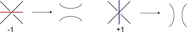
Figure 1. Markers and associated smoothings.

By $D_{s}$ we denote the system of circles in the diagram obtained by smoothing all crossings of $D$ according to the markers of the state $s$, for example see Figure 2b. Let $|D_{s}|$ denote the number of circles in state $D_{s}$.

Definition 2.2.

[PPS]  Let $D$ be a diagram of a link and $s$ its Kauffman state. We form a graph, $G_{s}(D)$, associated to $D$ and $s$ as follows. Vertices of $G_{s}(D)$ correspond to circles of $D_{s}$. Edges of $G_{s}(D)$ are in bijection with crossings of $D$ and an edge connects given vertices if the corresponding crossing connects circles of $D_{s}$ corresponding to the vertices, see Figures 2, 6, 7, 4. As in the case of the Tait graph, $G_{s}(D)$ can be turned into a signed graph, with the sign of an edge $e(p)$ associated with the crossing $p\in D$ equal to the sign of the marker of the Kauffman state $s$ at that crossing $p$ (notice that we will not be working with signed graphs in this paper).

The Kauffman bracket polynomial of a diagram $D$, $<D>_{(\mu,A,B)}\in Z[\mu,A,B]$ is defined by:

1. $<U_{n}>=\mu^{n-1}$, where $U_{n}$ is the trivial diagram of $n$ components.

2. $\langle D_{\parbox{14.22636pt}{\psfig{}}}\rangle=A\langle D_{\parbox{14.22636pt}{\psfig{}}}\rangle+B\langle D_{\parbox{14.22636pt}{\psfig{}}}\rangle$

From this we obtain the state sum formula:

$$<D>_{(\mu,A,B)}=\sum_{s}A^{|s^{-1}(1)|}B^{|s^{-1}(-1)|}\mu^{|D_{s}|-1}.$$

In order to have invariance of the Kauffman bracket polynomial under regular isotopy (i.e. Reidemeister moves $R_{2}$ and $R_{3}$) we need $B=A^{-1}$ and $\mu=-A^{2}-A^{-2}$.

In this notation the Kauffman bracket polynomial of $D$ is given by the state sum formula: $<D>=\sum_{s}A^{\sigma(s)}(-A^{2}-A^{-2})^{|D_{s}|-1}$, where $\sigma(s)=|s^{-1}(1)|-|s^{-1}(-1)|=\sum_{p}s(p)$ is the number of positive markers minus the number of negative markers in the state $s$.

The unreduced Kauffman bracket $[D]$ is defined as $[D]=(-A^{2}-A^{-2})<D>$, thus:

$$[D]=\sum_{s}A^{\sigma(s)}(-A^{2}-A^{-2})^{|D_{s}|}.$$

Figure 2. A minimal diagram of the Whitehead link (a), $D_{s_{-}}$ and $D_{s_{+}}$ in (b), and the corresponding graphs $G_{s_{-}}$ and $G_{s_{+}}$ in (c).

Before we move to the polynomial invariants of graphs we describe classes of knots and links we will be analyzing in this paper, and classify corresponding graphs.

Definition 2.3.

1. In the language of graphs, the diagram $D$ is s-adequate if the graph $G_{s}(D)$ has no loops.

2. The girth of a state $\ell(s)$ is the girth of the graph $G_{s}(D)$, i.e. the length of the shortest cycle in $G_{s}(D)$ (in the case $G$ is a forest we define $\ell(s)=\infty$). Thus $D$ is s-adequate if $\ell(s)>1$. Similarly, $D$ is strongly $s$-adequate if $\ell(s)>2$.

3. The $s_{+}$ Kauffman state is a constant function sending all crossings to $+1$, and $s_{-}$ to $-1$. We say that $D$ is $+$-adequate if it is $s_{+}$-adequate and that is $-$-adequate if it is $s_{-}$-adequate. Similarly, $D$ is strongly $+$-adequate if it is strongly $s_{-}$-adequate, and $D$ is strongly $-$-adequate if it is strongly $s_{+}$-adequate.

Figure 2 shows a diagram of a Whitehead link $D=D_{Wh}$, its $s_{-}$ smoothings (and $D_{s_{-}}$), $s_{+}$ smoothing (and $D_{s_{+}}$), and their graphs $G(D)=G_{s_{-}}(D)$ and $(\bar{D})=G_{s_{+}}(D)$. Notice that $D_{Wh}$ is strongly $-$-adequate, i.e., $G(\bar{D})=G_{s_{+}}(\bar{D})=G_{s_{-}}(D)$ is a simple graph.

2.2. The Kauffman bracket polynomial of graphs $[G]_{(\mu,A,B)}$

When we translate the Kauffman bracket polynomial of diagrams $[D]_{(\mu,A,B)}$ to graphs we obtain a version of the Tutte polynomial as explained below.

Definition 2.4.

The Kauffman bracket polynomial $[G]=[G]_{(\mu,A,B)}$ of the graph $G$ ($[G]\in Z[\mu,A,B]$) is defined inductively by the following formulas:

1. $[U_{n}]=\mu^{n}$, where $U_{n}$ is the discrete graph on $n$ vertices.

2. $[G]=A[G-e]+B[G//e]$ where $G//e=G/e$ if $e$ is not a loop, and if $e$ is a loop, then $G//e$ is defined to be the graph obtained from $G-e$ by adding an isolated vertex.

The Kauffman bracket satisfies the following state sum formula:

Lemma 2.5.

$$[G]=\sum_{s\in 2^{E(G)}}\mu^{p_{0}([G:s])+p_{1}([G:s])}A^{|E(G)-s|}B^{|s|}$$

where the state $s$ is an arbitrary set of edges of $G$, including the empty set, and $G-s$ denotes a graph obtained from $G$ by removing all edges contained in $s$.

The following formula expresses the relation between the Kauffman bracket and Tutte polynomial of a graph $G$.

Proposition 2.6.

The following identity holds

$$[G]_{(\mu,A,B)}=\mu^{p_{0}(G)}A^{p_{1}(G)}B^{E(G)-p_{1}(G)}\chi(G;x,y)$$

where $x=\frac{B+\mu A}{B}$ and $y=\frac{A+\mu B}{A}$.

2.3. Khovanov homology via enhanced states chain complex

Convenient way of defining Khovanov homology, as noticed by Viro [Vi1, Vi2], is to consider enhanced Kauffman states.

Definition 2.7.

An enhanced Kauffman state $S$ of an unoriented framed link diagram $D$ is a Kauffman state $s$ with an additional assignment of $+$ or $-$ sign to each circle of $D_{s}.$

The Kauffman bracket polynomial can be expressed as a sum of monomials using enhanced states which is important in our approach to defining Khovanov homology. We have $[D]=(-A^{2}-A^{-2})<D>=\sum_{S}(-1)^{\tau(S)}A^{\sigma(s)+2\tau(S)}$, where $\tau(S)$ is the number of positive circles minus the number of negative circles in the enhanced state $S$ (notice, that $\tau(S)\equiv|D_{s}|\,\mathrm{mod}2$).

Definition 2.8 (Khovanov chain complex).

Let ${\mathcal{S}}(D)$ denote the set of enhanced Kauffman states of a diagram $D$, and let ${\mathcal{S}}_{i,j}(D)$ denote the set of enhanced Kauffman states $S$ such that $\sigma(S)=i$ and $\sigma(S)+2\tau(S)=j$. We call $i$ a homology grading and $j$ a Kauffman bracket grading.

1. The group ${\mathcal{C}}(D)$ (resp. ${\mathcal{C}}_{i,j}(D)$) is the free abelian group freely generated by ${\mathcal{S}}(D)$ (resp. ${\mathcal{S}}_{i,j}(D)$). ${\mathcal{C}}(D)=\bigoplus_{i,j\in{\mathbb{Z}}}{\mathcal{C}}_{i,j}(D)$ is a bigraded free abelian group.

2. For a link diagram $D$ with ordered crossings, we define the chain complex $({\mathcal{C}}(D),d)$ where $d=\{d_{i,j}\}$ and the differential $d_{i,j}:{\mathcal{C}}_{i,j}(D)\to{\mathcal{C}}_{i-2,j}(D)$ satisfies $d(S)=\sum_{S^{\prime}}(-1)^{t(S:S^{\prime})}[S:S^{\prime}]S^{\prime}$ with $S\in{\mathcal{S}}_{i,j}(D)$, $S^{\prime}\in{\mathcal{S}}_{i-2,j}(D)$, and $[S:S^{\prime}]$ equal to $0$ or $1$. $[S:S^{\prime}]=1$ if and only if markers of $S$ and $S^{\prime}$ differ exactly at one crossing, call it $v$, and all the circles of $D_{S}$ and $D_{S^{\prime}}$ not touching $v$ have the same sign. Furthermore, $t(S:S^{\prime})$ is the number of negative markers assigned to crossings in $S$ bigger than $v$ in the chosen ordering.

3. The Khovanov homology of the diagram $D$ is defined to be the homology of the chain complex $({\mathcal{C}}(D),d)$; $H_{i,j}(D)=ker(d_{i,j})/d_{i+2,j}({\mathcal{C}}_{i+2,j}(D))$. The Khovanov cohomology of the diagram $D$ is defined to be the cohomology of the chain complex $({\mathcal{C}}(D),d)$.

Khovanov proved that his homology is a topological invariant. $H_{i,j}(D)$ is preserved by the second and the third Reidemeister moves and $H_{i+1,j+3}(r_{+1}(D))=H_{i,j}(D)=H_{i-1,j-3}(r_{-1}(D))$. Where $r_{+1}(\parbox{22.76228pt}{\psfig{height=17.07182pt}})=$ $(\parbox{28.45274pt}{\psfig{height=17.07182pt}})$ and $r_{-1}(\parbox{22.76228pt}{\psfig{height=17.07182pt}})=$ $(\parbox{28.45274pt}{\psfig{height=17.07182pt}})$.

With the notation we have introduced before, we can write the formula for the Kauffman bracket polynomial of a link diagram in the following form:

$$[D] = \sum_{j}A^{j}(\sum_{i}(-1)^{\frac{j-i}{2}}\sum_{S\in S_{i,j}}1)$$

$$= \sum_{j}A^{j}(\sum_{i}(-1)^{\frac{j-i}{2}}dimC_{i,j})=\sum_{j}A^{j}\chi_{i,j}(C_{*,j}),$$

where $\chi_{i,j}(C_{*,j})=\displaystyle{\sum_{\begin{smallmatrix}i:\,j\equiv i\\ (mod\,2)\end{smallmatrix}}}(-1)^{\frac{j-i}{2}}(dimC_{i,j})$ is a slightly adjusted Euler characteristic of the chain complex $C_{*,j}$ ($j$ fixed). This explains that Khovanov homology categorifies the Kauffman bracket polynomial, as well as the Jones polynomial.

2.4. Khovanov type functor on the category of graphs

The chromatic graph cohomology was introduced in [HR], as a comultiplication free version of the Khovanov cohomology of alternating links, where alternating link diagrams are translated to plane graphs (Tait graphs). Moreover, this homology theory is a categorification of the chromatic polynomial of a graph.

The chromatic polynomial of a graph counts the number of its proper vertex colorings using no more than a given number of colors, so that adjacent vertices have different colors. The analogy with the Khovanov homology construction is almost complete: instead of Kauffman states we use subgraphs $[G:s]$, containing all vertices in $G$ and $i$ edges in $s\subseteq E$. Analogously to the enhanced Kauffman states, we label connected components of a graph $[G:s]$ by either $1$ or $x$, the generators of algebra ${\mathcal{A}}_{2}={\mathbb{Z}}/(x^{2})$. The number of circles in the Kauffman state $|D_{s}|$ corresponds to the number of connected components $k(s)$ of the graph $[G:s]$ containing all vertices in $G$ and $i$ edges in $s\subseteq E$. Now, we consider the following state sum formula for the chromatic polynomial:

$$\chi_{G}(\lambda) = \displaystyle{\sum_{i\geq 0}(-1)^{i}\sum_{s\subseteq E,|s|=i}\lambda^{k(s)}}$$

$$= \displaystyle{\sum_{i,j\geq 0}(-1)^{i}\lambda^{j}\sharp\{s\subseteq E||s|=i,k^{\prime}([G:s])=j\}}.$$

where $k^{\prime}([G:s])$ denotes the number of components of $[G:s]$ labeled by $x$. Cochain groups are spanned by all subgraphs $[G:s]$, with each of $k([G:s])=j$ components labeled by either $1$ or $x$, with exactly $j$ components labeled by $x$.

The differential takes an enhanced state, i.e. labeled subgraph $[G:s]$ into a state $[G:s]^{\prime}$ where $S^{\prime}=S\cup{e}$, $e\in E\setminus S$. Components of the obtained state are labeled using multiplication rules in ${\mathcal{A}}_{2}$: if two different components are merged new label is a product of the old ones, otherwise, if a cycle is closed it is just an identity.

Definition 2.9.

Given commutative algebra ${\mathcal{A}}_{2}$ we define the chromatic cochain complex and chromatic cohomology of a graph $G=(V(G),E(G))$ with $V(G)$ set of vertices and $E(G)$ the set of edges in the following way:

1. The cochain group $C^{i}(G)=\displaystyle{\bigoplus_{|s|=i,s\subset E(G)}C^{i}_{s}(G)},$ with $C^{i}_{s}(G)={\mathcal{A}}^{k(s)}$ where $k(s)$ denotes the number of components of the graph $[G:s]$ which is the subgraph of $G$ containing all vertices of $G$ and edges in $s.$

   Assume that the edges of $G$ are ordered. For a given state $s$ and the edge $e\in E\setminus s$, let $t(s,e)$ equal to the number of edges in $s$ less than $e$ in the chosen ordering. The cochain map $d^{i}:C^{i}(G)\to C^{i+1}(G)$ is a sum

   $$d^{i}=\sum_{e\notin s}(-1)^{t(s,e)}d_{e}^{i}$$

   where the map $d_{e}^{i}$ depends on whether $e$ connects different components of $[G:s]$ or it connects vertices in the same component of $[G:s].$ In the last case we assume $d_{e}^{i}$ to be the identity (or alternatively zero map [HR]). If $e$ connects different components of $[G:s]$, say $i-th$ and $j$-th, $i<j$ then: $d_{e}^{i}(a_{1},a_{2},\ldots,a_{k(s)-1})=(a_{1},a_{2},\ldots,a_{i}a_{j},\ldots,a_{j-1},a_{j+1},\ldots,a_{k(s)-1})$.

2. We define the chromatic cohomology denoted by $H^{*}(G)$ as the cohomology of the above chromatic cochain complex.

The chromatic graph cohomology of a graph with a loop is always equal to zero (the chromatic polynomial as well) since the chain complex can be presented as a cone of two isomorphic chain complexes.

In this setting it is easier to work with the chain complex, similar to the classical homology theories. Therefore we perform concrete calculations in the chromatic graph homology setting and then use the universal coefficient theorem (see Proposition 2.10) to translate the results to the chromatic graph cohomology.

Proposition 2.10.

If the homology groups $H_{n}$ and $H_{n-1}$ of a chain complex $C$ of free abelian groups are finitely generated then

$$H^{n}(C;{\mathbb{Z}})=H_{n}(C;{\mathbb{Z}})/\mathrm{tor}(H_{n}(C;{\mathbb{Z}}))\oplus\mathrm{tor}(H_{n-1}(C;{\mathbb{Z}})).$$

In particular, we use the following identities:

• $H^{0,v-1}_{{\mathcal{A}}_{2}}(G)=H_{0,v-1}^{{\mathcal{A}}_{m}}(G)/tor(H_{0,v-1}^{{\mathcal{A}}_{2}}(G))$,

• $H^{1,v-1}_{{\mathcal{A}}_{2}}(G)=H_{1,v-1}^{{\mathcal{A}}_{2}}(G)\oplus tor(H_{0,v-1}^{{\mathcal{A}}_{2}}(G))$ and

• $H_{1,v-1}^{{\mathcal{A}}_{2}}(G)=ker(C_{1,v-1}^{{\mathcal{A}}_{2}}(G)\to C_{0,v-1}^{{\mathcal{A}}_{2}}(G))$ is a free abelian group.

The chromatic graph cohomology of a graph $G=(V(G),E(G))$ over algebra ${\mathcal{A}}_{2}$ is equivalent to the homology with chain groups defined as in the standard graph homology and the boundary map defined by $\partial(e)=\partial(\overrightarrow{V_{1}V_{2}})=V_{1}+V_{2}$ where $e=(V_{1},V_{2})\in E$. As a corollary we get the following lemma from [PPS]:

Proposition 2.11.

Let G be a connected simple graph, then:

(3) $$H_{0,v-1}^{{\mathcal{A}}_{2}}(G)=\left\{\begin{array}[]{ll}\mathbb{Z},&\hbox{if G is a bipartite graph;}\\ \mathbb{Z}_{2},&\hbox{if G has an odd cycle.}\\ \end{array}\right.$$

Consider the category of finite graphs in which finite graphs are objects and $Mor(H,G)$) are graph embeddings between $H$ and $G$ (for simplicity we assume that for a morphism $f:H\to G$, $f(H)$ is a spanning graph, that is, it contains all vertices of $G$). To every graph we associate its chain complex $\{C_{i,j}(G)\}$, moreover any $f:H\rightarrow G$ induces the chain map $f_{\#}:\{C_{i,j}(H)\}\to\{C_{i,j}(G)\}$. We obtain in such a way a functor from the category of finite graphs to the category of graded chain complexes, and further to the category of bi-graded groups $\{H_{i,j}(G)\}$. In a standard way we consider the morphism $\alpha$ of $H$ in $G$ and related short exact sequence of chain complexes

$$0\to C_{i,j}(H)\to C_{i,j}(G)\to C_{i,j}(G,H)\to 0$$

where $C_{i,j}(G,H)=C_{i,j}(G)/C_{i,j}(H)$. Finally, we obtain the related long exact sequence of homology:
  $\displaystyle\ldots$ $\displaystyle\to H_{i,j}(H)\to H_{i,j}(G)\to H_{i,j}(G,H)\to H_{i-1,j}(H)\to\ldots$ $\displaystyle\ldots$ $\displaystyle\to H_{1,j}(G)\to H_{1,j}(G,H)\to H_{0,j}(H)\to H_{0,j}(G)\to H_{0,j}(G,H)\to 0$

Proposition 2.12.

Let $T$ be a spanning tree of a connected graph $G$, then

1. $H_{*,*}(T)=H_{0,v-1}(T)\oplus H_{0,v}(T)={\mathbb{Z}}[0]\{v-1\}\oplus{\mathbb{Z}}[0]\{v\}$.

2. Homology is supported on two diagonals, $H_{i,j}(G)=0$ for $i+j\neq v,v-1$, and the torsion is trivial except possibly for $i+j=v-1$: $\mathrm{tor}H_{i,j}(G)=0$ for $i+j\neq v-1$.

3. $H_{i,j}(G)=H_{i,j}(G,T)$ if $i>1$ or $i=1$ and $j\neq v-1.$ In particular, $H_{1,v-2}(G)=H_{1,v-2}(G,T).$

Proof.

• Let $G_{1}*G_{2}$ denote one–vertex product of graphs and $K_{n}$ the complete graph on $n$ vertices. Adding a loop loop $K_{1}$ to a graph $G$ (see [HR]) on the level of knots, corresponds to applying first Reidemeister move to the knot. Part (i) is the special case of the fact that Khovanov homology of links is shifted under the first Reidemeister move $H_{i,j}(G*K_{1})=H_{i,j+1}(G)$.

• Part (ii) reflects the fact that Khovanov homology of alternating links lies on two adjacent diagonals [Lee]. The proof uses the long exact sequence of homology using smoothings in a link case and deleting–contracting in the graph case (see [HR, AP]).

• The third part follows from parts (i) and (ii) by applying the long exact sequence of the pair $(G,T)$.

∎

2.5. Correspondence between Khovanov and chromatic graph homology

Based on [HPR, Pr2] we state the following Proposition 2.13 that establishes the relation between graph cohomology and classical Khovanov homology of alternating links (in Viro [Vi1] notation). Proposition 2.13 is generalized in Proposition 4.7.

Proposition 2.13.

Let $D$ be the diagram of an unoriented framed alternating link and let $G=G_{s_{-}}(D)$. Let $\ell$ denote the girth of $G$, that is, the length of the shortest cycle in $G$. For all $i<\ell-1$, we have:

$$H^{i,j}_{{\mathcal{A}}_{2}}(G)\cong H_{a,b}(D)$$

where $a=E(G)-2i$, $b=E(G)-2v(G)+4j$ and $H_{a,b}(D)$ are the Khovanov homology groups of the unoriented framed link defined by $D$, as explained in Definition 2.7 based on [Vi1].

Furthermore, $tor(H^{i,j}_{{\mathcal{A}}_{2}}(G))=tor(H_{a,b}(D))$ for $i=\ell-1$.

Theorem 2.14.

[PPS] Let $G$ be a simple graph then

1. $H^{0,v-1}_{{\mathcal{A}}_{2}}(G)={\mathbb{Z}}^{p_{0}^{bi}}$, where $p_{0}^{bi}$ is the number of bipartite components of $G$.

2. $H^{1,v-1}_{{\mathcal{A}}_{2}}(G)={\mathbb{Z}}^{p_{1}-(p_{0}-p_{0}^{bi})}\oplus{\mathbb{Z}}_{2}^{p_{0}-p_{0}^{bi}}$, where $p_{0}$ is the number of components of $G$ and $p_{1}=rank(H_{1}(G,{\mathbb{Z}}))=|E|-v+p_{0}$ is the cyclomatic number of $G$.

3. The Main Lemma and chromatic graph homology $H_{1,v-2}$

Next we compute $H_{1,v-2}(G)$ for any connected graph $G$, hence $H^{2,v-2}(G)$ for any graph $G$ and, eventually, $H_{n-4,n+|D_{s_{+}}|-8}(D)$ for a corresponding $+$-adequate link diagram.

Lemma 3.1 (Main Lemma).

If $G$ is a connected simple graph, i.e., of girth $l(G)\geq 3$, then:

1. $H_{1,v-2}(G)={\mathbb{Z}}_{2}^{p_{1}(G)}$, if G is bipartite.

2. $H_{1,v-2}(G)={\mathbb{Z}}_{2}^{p_{1}(G)-1}\oplus{\mathbb{Z}}$, if G has an odd cycle.

Proof.

Since $H_{1,v-2}(G)=H_{1,v-2}(G,T)$, for any spanning tree $T$ of $G$, Proposition 2.12, we focus on computing $H_{1,v-2}(G,T)$. We assume that both edges and vertices are ordered, although results do not depend on it. To make the proof more comprehensible we introduce the following notation. Let $\rho(v,w)$ denote the distance between vertices $v,w\in V(T)$, equal to the length of the shortest path connecting them in $T$. If $(\partial_{0}(e),\partial_{1}(e))$ denotes endpoints of the $e$ edge in $G$, we use the short notation $\rho(e_{i})=\rho(\partial_{0}(e_{i}),\partial_{1}(e_{i})).$ In particular, $\rho(e_{i})$ is odd if $e$ closes an even cycle in $T\cup e_{i}$, and $\rho(e_{i})$ is even if $e$ closes an odd cycle in $T\cup e_{i}$. We also use $\rho(e_{i},e_{j})$ to denote the distance between $e_{i}$ and $e_{j}$ in $T\cup e_{i}\cup e_{j}$, or equivalently, as the minimal distance between endpoints of $e_{i}$ and endpoints of $e_{j}$ in $T$.

Let $e_{1},...,e_{p_{1}}$ be the edges in $E(G\setminus T)$ where $p_{1}(G)$ is the cyclomatic number of $G$, $p_{1}(G)=|E(G)|-|E(T)|=|E(G)|-|V(G)|+1$.

The chain group $C_{1,v-2}(G,T)$ is freely generated by enhanced states $(e_{i},v_{j})$ where the component of the graph $[G:e_{i}]$ containing the vertex $v_{j}$ has the label $1$ (all other labels are $x$). If the vertex $v_{j}$ is the endpoint of $e_{i}$ we use short notation $(e_{i},1)$ for an enhanced state $(e_{i},\partial_{0}(e_{i}))=(e_{i},\partial_{1}(e_{i}))$.

Notice that $H_{0,v-2}(G,T)=0=C_{0,v-2}(G,T)$ since $C_{0,v-2}(G)=C_{0,v-2}(T)$. Therefore, $ker(d:C_{1,v-2}(G,T)\rightarrow C_{0,v-2}(G,T))=C_{1,v-2}(G,T)$ so:

$$H_{1,v-2}(G,T)=C_{1,v-2}(G,T)/d(C_{2,v-2}(G,T)).$$

The chain group $C_{2,v-2}(G,T)$ has two types of free generators (enhanced states):

• pairs $(e_{i},e)$ where $e\in E(T)$ generating the subgroup of $C_{2,v-2}(G,T)$ denoted by $C^{\prime}$ and

• pairs $(e_{i},e_{j})$ generating the subgroup $C^{\prime\prime}.$

Let us first compute $C_{1,v-2}(G,T)/d(C^{\prime})$. For any edge $e\in T$,

$$d(e_{i},e)=\pm((e_{i},\partial_{1}(e))+(e_{i},\partial_{0}(e)))$$

yields the following relation in homology $(e_{i},\partial_{1}(e))=-(e_{i},\partial_{0}(e)).$ Hence, we eliminate all generators of $C_{1,v-2}(G,T)$ except pairs $(e_{i},\partial_{0}(e_{i}))$, satisfying relations

$$(e_{i},\partial_{1}(e_{i})) = (-1)^{\rho(\partial_{0}(e_{i}),\partial_{1}(e_{i}))}(e_{i},\partial_{0}(e_{i})){\rm\,that\,is}$$

$$(e_{i},1) = (-1)^{\rho(e_{i})}(e_{i},1).$$

Thus $C_{1,v-2}(G,T)/d(C^{\prime})={\mathbb{Z}}_{2}^{k_{odd}}\oplus{\mathbb{Z}}^{p_{1}-k_{odd}}$, where $k_{odd}$ is the number of edges $e_{i}$ with $\rho(e_{i})$ odd.

Next, we compute $(C_{1,v-2}(G,T)/d(C^{\prime}))/d(C^{\prime\prime})$. For an enhanced state $(e_{i},e_{j})$ we have:

(5) $$d(e_{i},e_{j})=\pm((e_{i},\partial_{0}(e_{j}))+(e_{i},\partial_{1}(e_{j}))-(e_{j},\partial_{0}(e_{i}))-(e_{j},\partial_{1}(e_{i})))$$

The relation in $C_{1,v-2}(G,T)/d(C^{\prime})$ corresponding to Equation 5 can be written as

(6) $$(e_{i},1)(1+(-1)^{\rho(e_{j})})=\varepsilon((e_{j},1)(1+(-1)^{\rho(e_{i})}),$$

where $\varepsilon=\pm 1$, or more precisely $\varepsilon=(-1)^{\rho(\partial_{0}(e_{i}),\rho(\partial_{0}(e_{j}))}$. We analyze this relation in more detail, based on the types of enhanced states generating $C^{\prime\prime}$. Depending on the parity of $\rho(e_{i},e_{j})$ we get three different types of generators of $C^{\prime\prime}$:

1. $(e_{i},e_{j})$ such that both $\rho(e_{i})$ and $\rho(e_{j})$ are odd generate the subgroup $C^{\prime\prime}_{odd}$

2. $(e_{i},e_{j})$ where exactly one of $\rho(e_{i})$ and $\rho(e_{j})$ is odd generate the subgroup $C^{\prime\prime}_{mixed}$

3. $(e_{i},e_{j})$ such that both $\rho(e_{i})$ and $\rho(e_{j})$ are even generate the subgroup $C^{\prime\prime}_{even}$

In the first case $C^{\prime\prime}_{odd}$, both sides of Equation(5) are equal to $0$, so there are no new relations in $C_{1,v-2}(G,T)/d(C^{\prime})$. If a graph $G$ is bipartite $\rho(e_{i})$ is always odd, $C_{2,v-2}(G,T)$ is generated by $C^{\prime}$ and $C^{\prime\prime}_{odd},$ so Part (i) of Main Lemma is proven.

In the second case, Equation (6) reduces to the equation $2(e_{i},1)=0$ which already holds in $C_{1,v-2}(G,T)/d(C^{\prime})$.

Finally, consider the third case when $2(e_{i},1)=\varepsilon 2(e_{j},1)$, or more precisely

(7) $$2((e_{i},1)-(-1)^{\rho(e_{i},e_{j})}(e_{j},1)))=0.$$

To conclude the proof of part (ii), let $e_{1},..,e_{k}$ be edges of $G\setminus T$ with odd $\rho(e_{i}),$ and $e_{k+1},...,e_{p_{1}}$ be the remaining edges, i.e. edges with $\rho(e_{i})$ even. Graph $H$ obtained by adding $e_{1},..,e_{k}$ to the tree $T$ is a bipartite graph, so we know that

$$H_{1,v-2}(H,T)=C_{1,v-2}(H,T)/d(C^{\prime})=\{\{(e_{i},1)\}_{i=1}^{k}\ |\ 2(e_{i},1)=0\}={\mathbb{Z}}_{2}^{k},$$

and that $H_{1,v-2}(G,T)=H_{1,v-2}(H,T)/C^{\prime\prime}_{even}.$ Observe now that for $e_{i},e_{j}$ in $E(G)\setminus E(H)$ the relation (7) follows from relations $2((e_{i},1)-(-1)^{\rho(e_{i},e_{k+1})}(e_{k+1},1))=0$ and $2((e_{j},1)-(-1)^{\rho(e_{j},e_{k+1})}(e_{k+1},1))=0$ since $\rho(e_{i},e_{j})\equiv\rho(e_{i},e_{k+1})+\rho(e_{j},e_{k+1})(\mathrm{mod}2)$. Hence, $H_{1,v-2}(G,T)$ is generated by
$(e_{1},,...,e_{k},e_{k+1},(e_{k+2}-(-1)^{\rho(e_{k+2},e_{k+1})}(e_{k+1},1)),\ldots,(e_{p_{1}}-(-1)^{\rho(e_{p_{1}},e_{k+1})}(e_{k+1},1))$, where $e_{k+1}$ is an infinite cyclic element and all other generators have order $2$. The proof of Main Lemma is completed. ∎

As a corollary we get the following main result.

Theorem 3.2.

1. If $G$ is a connected simple graph containing $t_{3}$ triangles, then:

2. $H_{1,v-2}(G)=\left\{\begin{array}[]{ll}{\mathbb{Z}}_{2}^{p_{1}(G)},&\hbox{if G is bipartite;}\\ {\mathbb{Z}}_{2}^{p_{1}(G)-1}\oplus{\mathbb{Z}},&\hbox{if G has an odd cycle.}\\ \end{array}\right.$

3. $H_{2,v-2}(G)=\left\{\begin{array}[]{ll}{\mathbb{Z}}^{{p_{1}\choose 2}-t_{3}},&\hbox{if G is bipartite;}\\ {\mathbb{Z}}^{{p_{1}\choose 2}-t_{3}+1},&\hbox{if G has an odd cycle.}\\ \end{array}\right.$

4. $H^{1,v-2}(G)=\left\{\begin{array}[]{ll}0,&\hbox{if G is bipartite;}\\ {\mathbb{Z}},&\hbox{if G has an odd cycle.}\\ \end{array}\right.$

5. $H^{2,v-2}(G)=\left\{\begin{array}[]{ll}Z_{2}^{p_{1}}\oplus Z^{{p_{1}\choose 2}-t_{3}},&\hbox{G is bipartite;}\\ Z_{2}^{p_{1}-1}\oplus Z^{{p_{1}\choose 2}+1-t_{3}},&\hbox{if G has an odd cycle.}\\ \end{array}\right.$

Proof.

(1) follows from Main Lemma and Proposition 2.12(iii).
(2) Using Euler characteristic of chromatic graph cohomology in degree $j=v-2$ we get:

$$\mathrm{rank}H_{2,v-2}(G)-\mathrm{rank}H_{1,v-2}(G)=a_{v-2}$$

where $a_{v-2}$ denotes the coefficient of $q^{v-2}$ in the chromatic polynomial equal to:

(8) $$a_{v-2}={E\choose 2}-t_{3}-E(v-1)+{v\choose 2}={p_{1}\choose 2}-t_{3}.$$

Parts (3) and (4) follow directly from (1) and (2) by applying universal coefficient theorem ($H^{2,v-2}(G)=\mathrm{free}(H_{2,v-2}(G))\oplus\mathrm{tor}H_{1,v-2}(G)$, and $H^{1,v-2}(G)=\mathrm{free}(H_{1,v-2}(G)$). ∎

The restriction to connected graphs was made only for simplicity. Künnet formula is sufficient for recovering homology of the graph from the homology of the connected components (compare with [HR]). In fact, when computing the homology of a disjoint sum of graphs, $H^{**}(G_{1}\sqcup G)$, we can sometimes ignore the torsion part of the formula.

Corollary 3.3.

Let $G$, $G_{1}$ and $G_{2}$ denote arbitrary graphs, $G^{bi}$ all bipartite components of $G$, and $G^{nbi}=G-G^{bi}$ the remaining components of the graph $G$.

1. $H^{i,v-i}_{{\mathcal{A}}_{2}}(G_{1}\sqcup G_{2})=H^{**}_{{\mathcal{A}}_{2}}(G_{1})\otimes H^{**}_{{\mathcal{A}}_{2}}(G_{2})$ in bidegree $(i,v-i).$

2. If $G^{bi}$ and $G^{nbi}$ are simple graphs then:

   (9) $$H^{2,v-2}_{{\mathcal{A}}_{2}}(G^{bi}) = {\mathbb{Z}}_{2}^{p_{1}(G^{bi})}\oplus{\mathbb{Z}}^{{p_{1}(G)\choose 2}}$$

   (10) $$H^{2,v-2}_{{\mathcal{A}}_{2}}(G^{nbi}) = {\mathbb{Z}}_{2}^{p_{0}(G^{nbi})p_{1}(G^{nbi})-{p_{0}(G^{nbi})+1\choose 2}}\oplus{\mathbb{Z}}^{\alpha}$$

   where $\alpha={p_{1}(G^{nbi})+1\choose 2}-(p_{0}(G^{nbi})-1)p_{1}(G^{nbi})-{p_{0}(G^{nbi})+1\choose 2}.$

3. If $G$ is simple graph with $p_{0}(G)$ components then

   (11) $$\mathrm{tor}H^{2,v-2}_{{\mathcal{A}}_{2}}(G)={\mathbb{Z}}_{2}^{p_{1}(G^{bi})+p_{0}(G^{nbi})p_{1}(G)+{p_{0}(G^{nbi})+1\choose 2}}.$$

4. If $G$ is simple graph with $p_{0}(G)$ components then

   $$\mathrm{rank}H^{2,v-2}_{{\mathcal{A}}_{2}}(G)={{p_{1}(G)+1\choose 2}-\dim\mathrm{tor}H^{2,v-2}_{{\mathcal{A}}_{2}}(G)-t_{3}(G)}.$$

Proof.

1. Künneth formula yields the following formula for chromatic graph cohomology over ${\mathcal{A}}_{2}$

   (12) $$H^{i,j}(G_{1}\sqcup G_{2})=\bigg{(}\mathop{\bigoplus_{p+q=i}}_{s+t=j}H^{p,s}(G_{1})\otimes H^{q,t}(G_{2}))\oplus\mathop{(\bigoplus_{p+q=i+1}}_{s+t=j}H^{p,s}(G_{1})*_{Tor}H^{q,t}(G_{2}))\bigg{)}$$

   thus it suffices to show that

   $$\mathop{\bigoplus_{p+q=i+1}}_{s+t=j}H^{p,s}_{{\mathcal{A}}_{2}}(G_{1})*_{Tor}H^{q,t}_{{\mathcal{A}}_{2}}(G_{2})=0$$

   in bidegrees $(i,j)$ satisfying $i+j=v(G_{1}\sqcup G_{2})$.

   If $G$ is a connected graph

   • homology is supported in bidegrees $(i,j)$ satisfying $v(G)-1\leq i+j\leq v(G)$

   • torsion is supported in $(i,j)$ such that $i+j=v(G)$.

   By induction on the number of components and Künneth formula we get a well known fact (compare with [AP, HPR]) for an arbitrary graph $G$

   • homology is supported in bidegrees $(i,j)$ such that $v(G)-p_{0}(G)\leq i+j\leq v(G)$

   • torsion is supported $(i,j)$ such that $v(G)-p_{0}(G)+1\leq i+j\leq v(G)$.

   From the second inequality and the Künneth formula we are interested only in bidegrees satisfying $p+q+r+s=v(G_{1}\sqcup G_{2})+1=v(G_{1})+v(G_{2})+1.$ However, this implies that either $p+q\geq v(G_{1})$ or $s+t\geq v(G_{2})$, which contradicts the previous observation. Hence,

   $$\mathop{\bigoplus_{p+q=i+1}}_{s+t=j}H^{p,s}(G_{1})*_{Tor}H^{q,t}(G_{2})$$

   is trivial.

2. According to part (1) we have:

   $$H^{2,v(G_{1}\sqcup G_{2})-2}_{{\mathcal{A}}_{2}}(G_{1}\sqcup G_{2}) = H^{2,v(G_{1})-2}_{{\mathcal{A}}_{2}}(G_{1})\oplus H^{2,v(G_{2})-2}_{{\mathcal{A}}_{2}}(G_{2})\oplus$$

   $$\oplus (H^{1,v(G_{1})-1}_{{\mathcal{A}}_{2}}(G_{1})\otimes H^{1,v(G_{2})-1}_{{\mathcal{A}}_{2}}(G_{2})).$$

   We apply this formula inductively, using results from Theorem 3.2(iv) and Theorem 2.14, to obtain formulas (9) and (11). The intermediate step is computing $H^{2,v-2}_{{\mathcal{A}}_{2}}(G^{bi})$ assuming that $G^{bi}=G_{1}^{bi}\sqcup G_{2}^{bi}\sqcup\ldots\sqcup G^{bi}_{p_{0}(G^{bi})}$:

   $$H^{2,v-2}_{{\mathcal{A}}_{2}}(G^{bi})={\mathbb{Z}}_{2}^{p_{1}(G^{bi})}\oplus{\mathbb{Z}}^{{p_{1}(G^{bi})\choose 2}}$$

   using the identity ${p_{1}(G_{1})\choose 2}+...+{p_{1}(G_{p_{0}(G)})\choose 2}+\sum_{i<j}p_{1}(G_{i})p_{1}(G_{j})={p_{1}(G)\choose 2}$.

   Similarly, assuming that $G^{nbi}=G_{1}^{nbi}\sqcup G_{2}^{nbi}\sqcup\ldots\sqcup G^{nbi}_{p_{0}(G^{nbi})}$:

   $$H^{2,v-2}_{{\mathcal{A}}_{2}}(G^{nbi})={\mathbb{Z}}_{2}^{p_{0}(G^{nbi})p_{1}(G^{nbi})+{p_{0}(G^{nbi})+1\choose 2}}\oplus{\mathbb{Z}}^{\alpha}$$

   where $\alpha={p_{1}(G^{nbi})+1\choose 2}-(p_{0}(G^{nbi})-1)p_{1}(G^{nbi})-{p_{0}(G^{nbi})+1\choose 2}-t_{3}(G^{nbi}).$

3. Proof of part (3) follows from results in (2) and to complete the proof of part (4) notice that that for any simple graph $G$

   $$rank(free(H^{2,v(G)-2}(G)))+dim(tor(H^{2,v(G)-2}(G))))={p_{1}(G)+1\choose 2}-t_{3}(G).$$

∎

Corollary 3.4.

Let $K_{n}$ denote the complete graph with $n$ vertices. Then

$$H^{2,v-2}_{{\mathcal{A}}_{2}}(K_{n})={\mathbb{Z}}^{\frac{n(n-3)}{2}}\oplus{\mathbb{Z}}^{3{n\choose 4}+1-{n\choose 3}}$$

Corollary 3.5.

Let $W_{n}$ denote the wheel graph with $n+1$ vertices, i.e. the cone over an $n$-gon. Then

$$H^{2,v-2}_{{\mathcal{A}}_{2}}(W_{n})={\mathbb{Z}}_{2}^{n-2}\oplus{\mathbb{Z}}^{{n-1\choose 2}-n+1}$$

4. Adding comultiplication to chromatic graph cohomology

In order to make further use of correspondence between Khovanov and chromatic graph cohomology described in Subsection 2.5 and [AP, HPR, Pr2, PPS], we adjust the original definition by incorporating comultiplication in the differential. This modification extends the correspondence between Khovanov homology and chromatic graph cohomology to additional homological grading. In particular, this definition enables computing torsion in Khovanov homology in bidegree $(n-4,n+2|D_{s_{+}}|-8)$.

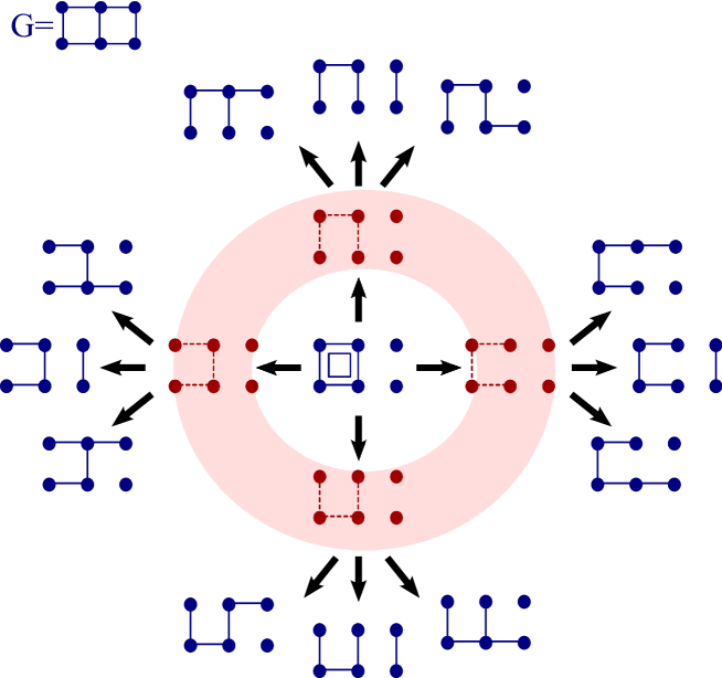
Figure 3. Examples of generators of ${}^{\Delta}C_{3}(G)$ (shown in red, dashed, in a shaded annulus) and ${}^{\Delta}C_{4}(G)$ (shown blue) for graph $G$ in the top left corner.

First, the chain complex is adjusted so that it can accommodate comultiplication. The original cochain groups contain a copy of algebra for each connected component in the graph $[G:s]$, see Definition 2.9. Cochain groups ${}^{\Delta}C^{i}(G)$ stay the same for $i<l(G)$, and trivial for $i>l(G)$. Modified cochain groups ${}^{\Delta}C^{i}(G)$ will contain a tensor product ${\mathcal{A}}_{2}\otimes{\mathcal{A}}_{2}$ instead of a single copy of algebra ${\mathcal{A}}_{2}$ for each state containing a closed cycle. Pictorially, the component containing a closed cycle is decorated by basis elements of a tensor product ${\mathcal{A}}_{2}\otimes{\mathcal{A}}_{2}$, see Figure 3. This description is formalized in the following definition.

Definition 4.1.

For a given graph $G$ of girth $l$, let ${}^{\Delta}C^{i,*}(G)$ denote modified chromatic chain groups defined in the following way:

1. ${}^{\Delta}C^{i,*}(G)\cong C^{i,*}(G)$ for $i<l$,

2. ${}^{\Delta}C^{i,*}(G)\cong\bigoplus_{|s|=i}{\mathcal{A}}_{2}^{\otimes(p_{0}([G:s])+p_{1}([G:s]))}$ for $i=l$,

3. ${}^{\Delta}C^{i,*}(G)=0$ for $i>l$.

Next, we introduce comultiplication in the differential the first time when adding an edge preserves the number of connected components of a graph, i.e. when it is closing shortest cycles. Let ${}^{\Delta}d_{s,e}$ denote the modified differential. If $p_{1}([G:s])=p_{1}([G:s\cup e])=0$, the differential stays the same ${}^{\Delta}d_{s,e}=d_{s,e}.$ If the edge $e$ we are adding is an internal edge of $[G:s]$ (i.e. $1=p_{1}([G:s\cup e])=p_{1}([G:s])+1$), the differential is determined by comultiplication in algebra ${\mathcal{A}}_{2}$, given by $\triangle(1)=(1\otimes x)+(x\otimes 1)$ and $\triangle(x)=x\otimes x$.

We have all necessary ingredients to define the differential.

Definition 4.2.

The differential map ${}^{\Delta}d^{i}(G):{}^{\Delta}C^{i}(G)\rightarrow{}^{\Delta}C^{i+1}(G)$ is defined by

$${}^{\Delta}d^{i}[G:s]=\sum_{e\in E(G)\setminus s}(-1)^{t(s,e)}d_{e}([G:s])$$

where $[G:s]\in{}^{\Delta}C^{i}(G)$ and $t(s,e)=|\{e^{\prime}\in s|e^{\prime}<e\}|$ for all $i<l(G)$. Let $c_{1},\ldots c_{k}$ denote the components of the state $[G:s].$ The definition of the map $d_{e}$ varies depending on whether the edge e is connecting two different components of $[G:s]$, say $c_{m}$ and $c_{n}$, $m<n$ or is closing a shortest cycle, which can happen only in degree $i=l(G)-1$:

1. If $|s|<l$, then $d_{e}([G:s])$ has one component less than $[G:s],$ say

   $$c_{1},\ldots,c_{m}\cup e\cup c_{n},\ldots c_{n-1},c_{n+1},\ldots,c_{k}.$$

   The label of the newly obtained component $c_{m}\cup e\cup c_{n}$ is equal to the product of labels of components being merged, $c_{m}$ and $c_{n}$. In other words, $d_{e}$ is given by the multiplication in algebra.

2. If $|s|=l$, then

   • if number of components of s is greater than that of $s\cup e$, then $d_{e}$ is the same as in the case (1).

   • if the number of components is preserved then $d_{e}([G:s])=(c_{1},\ldots,c_{m}\cup e,\ldots)$ and the closed component $c_{m}\cup e$ is decorated by $\Delta(c_{m})$.

3. If $|s|>l$, i.e if $p_{1}([G:s])\geq 1$, $d_{e}$ is a zero map.

Next, in order to have a degree-preserving differential we need to adjust the definition of degrees of basis elements of ${\mathcal{A}}_{2}\otimes{\mathcal{A}}_{2}$ obtained from comultiplication, according to the convention in Table 1. In general, the degree would be lowered by the cyclomatic number $p_{1}(G)$, but since we are closing the shortest cycle the adjustment is only by $1$.

Basis element	Degree
$1\otimes 1$	$-1$
$1\otimes x$, $x\otimes 1$	$0$
$x\otimes x$	$1$

Table 1. Degrees of basis elements in ${\mathcal{A}}_{2}\otimes{\mathcal{A}}_{2}$ coming from the comultiplication.

The cohomology ${}^{\Delta}H^{*,*}(G)$ of the modified bigraded cochain complex ${}^{\Delta}C(G)$ is also an invariant of all graphs.

Next we analyze the differences between the modified chromatic graph cohomology and the original one. In general, homology of these two complexes agree in homological degrees less than the girth of the graph $l(G)$.

Lemma 4.3.

For a loopless graph $G$, with $v$ vertices and girth $l(G)=l$, $C^{i}_{{\mathcal{A}}_{2}}(G)\cong C^{i}_{{\mathcal{A}}_{2}}(G)$ for $0\leq i<l$. Moreover, there exists an injective map $\alpha:C^{l}_{{\mathcal{A}}_{2}}(G)\rightarrow{}^{\Delta}C^{l}_{{\mathcal{A}}_{2}}(G)$, so homologies are isomorphic up to homological level $l-1$.

However, we are most interested in the bidegree $(l(G),v-l(G))$, in particular, $(2,v-2)$. The change in the definition is preserving $H^{2,v-2}_{{\mathcal{A}}_{2}}(G)$ for loopless graphs even if multiple edges are allowed. The proof of this fact relies on duality between the homology and cohomology and the following Lemma 4.4.

Lemma 4.4.

For a loopless graph $G$, with possible multiple edges, the following holds:

$$H_{1,v-2}^{{\mathcal{A}}_{2}}(G)\cong{}^{\Delta}H_{1,v-2}^{{\mathcal{A}}_{2}}(G)$$

Proof.

According to the original and modified definitions of chromatic graph homology, both chain groups and differentials agree on the zeroth and first level. Hence, we only need to analyze ${}^{\Delta}d_{2}$ and ${}^{\Delta}H_{2,v-2}(G)$ if graph $G$ has double or multiple edges. Under this assumption ${}^{\Delta}C_{2,v-2}(G)$ has more generators than ${}^{\Delta}C_{2,v-2}(G^{\prime})$, where $G^{\prime}$ denotes a simple graph obtained from $G$. Without loss of generality, denote the double edge by $e=(e_{1},e_{2})$. We have two different cases:

1. If $e$ has weight $x\otimes x$ of degree $1$, then all but one of the remaining vertices have labels $x$. Denote the special vertex by $v$ and the state by $(e(x\otimes x),v(1))$. The image of this state ${}^{\Delta}d_{2}(e,v)=(e_{1}(x),v(1))\pm(e_{2}(x),v(1))$ gives the relation $(e_{1}(x),v(1))=(e_{2}(x),v(1))$, so there are no new generators in homology.

2. If $e$ is labeled by $1\otimes x$ or $x\otimes 1$, both of degree zero, all of the remaining vertices have to be labeled by $x$ and ${}^{\Delta}d_{2}(e(1\otimes x))={}^{\Delta}d_{2}(e(x\otimes 1))=e_{1}(1)-e_{2}(1).$

Therefore $Im{}^{\Delta}d_{2}$ and $Imd_{2}$ impose the same relations on homology which completes the proof. ∎

Corollary 4.5.

For a loopless graph $G$ with $v$ vertices, $\mathrm{tor}H_{{\mathcal{A}}_{2}}^{2,v-2}(G)\cong\mathrm{tor}{}^{\Delta}H^{2,v-2}_{{\mathcal{A}}_{2}}(G)$.

Proposition 4.6.

For a connected graph $G$ with girth $l(G)=1$ homology group ${}^{\Delta}H_{0,v-1}(G)=0$, and $\mathrm{tor}{}^{\Delta}H^{1,v-1}(G)=0$.

Proof.

If $e_{\ell}$ denotes a loop in $G$ at the vertex $V$, notice that there is an epimorphism

$${}^{\Delta}d_{1}=d_{1}:{}^{\Delta}C_{1,v-1}(G)\to{}^{\Delta}C_{0,v-1}(G)$$

sending each generator of ${}^{\Delta}C_{1,v-1}(G)$ containing $e_{\ell}$ to a generator of ${}^{\Delta}C_{0,v-1}(G)$ with a label $1$ or $x$ at the vertex $V$, if $e_{\ell}$ had weight $1\otimes x$, $x\otimes 1$, or $x\otimes x$. Hence ${}^{\Delta}H_{0,v-1}^{{\mathcal{A}}_{2}}(G)=0$ and ${\tiny{}^{\Delta}}H^{1,v-1}_{{\mathcal{A}}_{2}}(G)$ is torsion free. ∎

Finally, we can compute the torsion in Khovanov homology in Proposition 4.8, according to the next Proposition 4.7.

Proposition 4.7.

Let $D$ be the diagram of an unoriented framed link $L$, $G=G_{s_{-}}(D)$ its associated graph, and $l=l(G)$ girth of a loopless graph. Then:

1. For all $i<\ell$, we have: ${}^{\Delta}H^{i,j}_{{\mathcal{A}}_{2}}(G)\cong H_{a,b}(D),$

2. For $i=\ell$ we have: $\mathrm{tor}({}^{\Delta}H^{i,j}_{{\mathcal{A}}_{2}}(G))=tor(H_{a,b}(D)),$

where $a=E(G)-2i$, $b=E(G)-2v(G)+4j$ and $H_{a,b}(D)$ are the Khovanov homology groups of the unoriented framed link $L$ defined by $D$.

Proposition 4.8.

Consider a link diagram $D$ with $n$ crossings. If $D$ is $+$-adequate and $G^{\prime}=G^{\prime}_{s_{+}}(D)$ a simple graph obtained from $G$, with $p_{0}(G)^{bi})$ bipartite components, $p_{0}(G^{nbi})$ non-bipartite components, $p_{0}(G)$ number of connected components and the cyclomatic number $p_{1}(G^{\prime})$, then

1. If $G^{\prime}(D)$ is connected then we get the result (2)

   $$\mathrm{tor}H_{n-4,n+2|D_{s_{+}}|-8}(D)=\left\{\begin{array}[]{ll}{\mathbb{Z}}_{2}^{p_{1}(G^{\prime}(D))-1},&\hbox{for $G^{\prime}(D)$ having an odd cycle;}\\ {\mathbb{Z}}_{2}^{p_{1}(G^{\prime}(D))},&\hbox{{for $G^{\prime}(D)$ a bipartite graph.}}\end{array}\right.$$

2. $$\mathrm{tor}H_{n-4,n+2|D_{s_{+}}|-8}(D)={\mathbb{Z}}_{2}^{p_{1}(G^{\prime})+p_{0}(G)^{nbi})p_{1}(G)-{p_{0}(G)^{nbi})+1\choose 2}}.$$

Figure 4. The link $8^{4}_{1}$ and the corresponding graph $G_{s_{+}}(8^{4}_{1}).$

Example 4.9.

The following example illustrates the strength of Proposition 4.8 with respect to the previous results. Consider the link $8^{4}_{1}$, shown in Figure 4 together with its graph $G(8^{4}_{1})=G_{s_{+}}(8^{4}_{1})$. Torsion $\mathrm{tor}H_{4,8}(8^{4}_{1})={\mathbb{Z}}_{2}$ in Khovanov homology of this link could not be detected by results of [AP], but can be obtained from Theorem 3.2(4) together with Proposition 4.8(1). More importantly, it answers the question raised in [AP], whether Theorem 3.2 of [AP] can be improved so that $H_{n-4,n+2|D_{s_{+}}|-8}(D)$ has $Z_{2}$ torsion for any $+$-adequate diagram with an even n-cycle ($n\geq 4$).

Our next goal is to find explicit formula for Khovanov homology $H_{n-2i,n+2|D_{s_{+}}|-4i}(D)$ for $i<\ell(G(D))$, and $\mathrm{tor}H_{n-2\ell(G(D)),n+2|D_{s_{+}}|-4\ell(G(D))}(D)$. We plan to use our method for computing elements of a categorification of skein modules of a product of a surface with the interval as defined in [APS].

5. Adequate positive braids

Results obtained in Section 3 can be used for finding torsion in Khovanov homology, in particular we find $2$-torsion for some positive $3$-braids.

Figure 5. The smallest non-alternating adequate knot $10_{152}.$

Notice that the smallest adequate non-alternating knot $10_{152}$ in Rolfsen’s table [Ro] corresponds to the positive minimal braid is $s_{1}^{3}s_{2}^{2}s_{1}^{2}s_{2}^{3}$, see Figure 5. The graph assigned to the Kauffman state with all negative resolutions $s_{-}$ has only multiple edges, so our method can not detect torsion, see Figure 6.

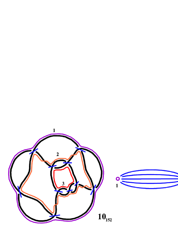
Figure 6. $s_{-}$ Kauffman state of $10_{152}$ and the corresponding graph.

Figure 7. $s_{+}$ Kauffman state of $10_{152}$ and the corresponding graph.

On the other hand, the graph corresponding to the state $s_{+}$ with all positive smoothings, contains triangles, hence, $H_{8,16}\,(10_{152})$ contains ${\mathbb{Z}}_{2}$, see Figure 7. More precisely,

$$\mathrm{tor}H_{8,16}(10_{152})={\mathbb{Z}}_{2}=\mathrm{tor}H_{6,12}(10_{152}).$$

This example can be generalized to positive and negative $3$-braids. In Proposition 5.1 we state the result for positive braids; the result for negative braids is analogous.

Proposition 5.1.

Let $\gamma=\sigma_{i_{1}}^{a_{1}}\sigma_{i_{2}}^{a_{2}}...\sigma_{i_{k}}^{a_{k}}$ be a positive $3$-braid such that $i_{j}\in\{1,2\}$, $i_{j}\neq i_{j+1}$, $a_{i}\geq 1$, and $\widehat{\gamma}$ a closure of $\gamma$. Then the following statements are true

1. The link diagram $\widehat{\gamma}$ is adequate if and only if $a_{j}\geq 2$ for every $0<j\leq k$.

2. If additionally $a_{j}\geq 3$, for some $j$ then the link diagram $\widehat{\gamma}$ has $Z_{2}$-torsion in Khovanov homology.

3. If part (1) holds and $\widehat{\gamma}$ is a knot or a link of 2 components, then (2) holds.

Proof.

Consider a standard diagram $\widehat{\gamma}$ of a positive $3$-braid $\gamma$. Since the diagram is positive, link is $+$-adequate. In this case graph $G_{s_{+}}$ has three vertices and only $2$-cycles, compare with Figure 6. On the other hand, the graph $G_{s_{-}}$ contains an $a_{i}$-gon for any $0<i\leq k$. In particular, if all $a_{i}\geq 2$, this graph has no loops, hence $\widehat{\gamma}$ is $-$-adequate. Furthermore, if at least one $a_{j}\geq 3$, than the girth of the corresponding graph $G_{s-}$ is at least $3$. According to Theorem 2.14 and Theorem 3.2 Khovanov homology of such $3$-braids contains $Z_{2}$-torsion. Part (3) follows from the fact that when all $a_{i}=2$, then $\widehat{\gamma}$ is a link of $3$ components. ∎

The weaker version of Proposition 5.1 holds for all positive $n$-braids.

Proposition 5.2.

Let $\gamma=\sigma_{i_{1}}^{a_{1}}\sigma_{i_{2}}^{a_{2}}...\sigma_{i_{k}}^{a_{k}}$ be a positive n-braid such that $a_{i}\geq 2$ for any $i$ then $\widehat{\gamma}$ is an adequate diagram. If additionally $a_{j}\geq 3$ for some $j$ then $\widehat{\gamma}$ has $Z_{2}$-torsion in Khovanov homology.

6. Conjectures

The main goal of this paper was to enhance our understanding of torsion in Khovanov homology. In order to do so, we have analyzed those gradings in chromatic graph cohomology that agree with Khovanov homology. This approach brought new insights about torsion that agree with the recent results by A. Shumakovitch [Sh3] stating that there is no other torsion except ${\mathbb{Z}}_{2}$ in Khovanov homology of alternating knots. Experimental results obtained using Shumakovitch’s software KhoHo, Knotscape by M. Thistlethwaite, and LinKnot by S. Jablan and the second author show that there are eight positive $15$-crossing knots whose $4$-braid diagrams are adequate, and which have $Z_{4}$ torsion in Khovanov homology.. We suspect that the order of torsion in Khovanov homology partially depends on the minimal braid index of a given link as stated in the following conjecture.

Conjecture 6.1.

PS braid conjecture

• Khovanov homology of a closed $3$-braid can have only $Z_{2}$ torsion.

• Khovanov homology of a closed $4$-braid cannot have an odd torsion.

• Khovanov homology of a closed $4$-braid can have only $Z_{2}$ and $Z_{4}$ torsion.

• Khovanov homology of a closed $n$-braid cannot have p-torsion for $p>n$ (p prime).

• Khovanov homology of a closed $n$-braid cannot have $Z_{p^{r}}$ torsion for $p^{r}>n$.

Note that we are stating these conjectures with various degrees of confidence. The case of $3$-braids were extensively tested using A. Shumakovitch software KhoHo, and P. Turner proved that Khovanov homology of $(3,q)$ torus links can contain only $2$-torsion [Lo, Tu]. In 2011, W. Gilliam [Gi] showed that only $Z_{2}$ torsion is possible in their Khovanov homology. D. Bar-Natan [BN] checked that $(n,4)$ torus knots have $Z_{4}$ torsion for $n=5,7,9,11$.

Example 6.2.

Till summer of 2012, only $5$-strand torus knots: ($6$,$5$), ($7$,$5$), ($8$,$5$) and ($9$,$5$) were known to have $Z_{5}$-torsion in Khovanov homology. We predicted that positive adequate $36$-crossing knot $K$ given by the closure of the braid $s_{1}^{2}s_{2}^{2}s_{1}^{3}s_{2}^{2}s_{1}s_{3}s_{2}^{2}s_{4}^{2}s_{3}s_{1}^{2}s_{2}^{2}s_{1}^{3}s_{2}^{3}s_{1}^{2}s_{3}s_{2}^{2}s_{4}^{3}s_{3}^{2}$ has $Z_{5}$ torsion, which was confirmed by A. Shumakovitch using JavaKh [BNG]. More precisely, we show that homology mod $5$ and mod $7$ have different ranks while homology mod $7$ and mod $11$ have the same ranks. The difference between Khovanov polynomials computed mod $5$ and mod $7$ (see Appendix) is strictly positive:

$$KH_{5}(K)-KH_{7}(K)=(t^{12}+t^{11})q^{51}+(t^{11}+t^{10})q^{47}.$$

This means that the rank of $5$-torsion is strictly greater than one of $7$-torsion, hence torsion of order $5$ exists at least in degrees $(12,51)$, and $(11,47)$.

Finally for ($8$,$7$) torus knot Bar-Natan computed Khovanov homology and showed that it contains $Z_{7}$, $Z_{5}$, $Z_{4}$, and $Z_{2}$-torsion but this $48$ crossing $7$-braid reaches the limits of current computational resources.

ACKNOWLEDGEMENTS
J.H. Przytycki was partially supported by the NSA-AMS 091111 grant and by NSF-DMS-1137422 grant. R. Sazdanović was fully supported by the Postdoctoral Fellowship at MSRI, Berkeley during the early stages of this project, and NSF 0935165 and AFOSR FA9550-09-1-0643 grants towards the end. We are profoundly thankful to the Mathematisches Forschungsinsitut Oberwolfach for providing us with unique computer facilities that made computations of Example 6.2 possible.

Appendix A Khovanov homology computations

We include Khovanov polynomials of positive adequate $36$-crossing knot $K$ given by the closure of the braid $s_{1}^{2}s_{2}^{2}s_{1}^{3}s_{2}^{2}s_{1}s_{3}s_{2}^{2}s_{4}^{2}s_{3}s_{1}^{2}s_{2}^{2}s_{1}^{3}s_{2}^{3}s_{1}^{2}s_{3}s_{2}^{2}s_{4}^{3}s_{3}^{2}$ computed over $Z_{5}$ and $Z_{7}$. Computations were done in JavaKh [BNG] by A. Shumakovitch using Mathematisches Forschungsinsitut Oberwolfach world-class computer facilities.

$$KH_{5}(K)=q^{31}t^{0}+q^{33}t^{0}+q^{35}t^{2}+q^{39}t^{3}+2q^{37}t^{4}+q^{39}t^{4}+2+q^{41}t^{5}+q^{43}t^{5}+q^{39}t^{6}+$$

$$2q^{41}t^{6}+2q^{43}t^{7}+2q^{45}t^{7}+4q^{41}t^{8}+3q^{43}t^{8}+q^{47}t^{8}+13q^{43}t^{9}+4q^{45}t^{9}+4q^{47}t^{9}+2q^{43}t^{10}+$$

$$29q^{45}t^{10}+14q^{47}t^{10}+q^{51}t^{10}+9q^{45}t^{11}+44q^{47}t^{11}+31q^{49}t^{11}+q^{51}t^{11}+2q^{45}t^{12}+34q^{47}t^{12}+$$

$$68q^{49}t^{12}+42q^{51}t^{12}+2q^{53}t^{12}+11q^{47}t^{13}+85q^{49}t^{13}+97q^{51}t^{13}+59q^{53}t^{13}+45q^{49}t^{14}+$$

$$159q^{51}t^{14}+142q^{53}t^{14}+63q^{55}t^{14}+137q^{51t^{1}5}+245q^{53}t^{15}+202q^{55}t^{15}+9q^{57}t^{15}+345q^{53}t^{16}+$$

$$5376q^{55}t^{16}+237q^{57}t^{16}+54q^{59}t^{16}+735q^{55}t^{17}+589q^{57}t^{17}+260q^{59}t^{17}+37q^{61}t^{17}+$$

$$1328q^{57}t^{18}+953q^{59}t^{18}+253q^{61}t^{18}+21q^{63}t^{18}+2040q^{59}t^{19}+1501q^{61}t^{19}+220q^{63}t^{19}+$$

$$9q^{65}t^{19}+2729q^{61}t^{20}+2149q^{63}t^{20}+173q^{65}t^{20}+2q^{67}t^{20}+2q^{61}t^{21}+3203q^{63}t^{21}+$$

$$2779q^{65}t^{21}+109q^{67}t^{21}+11q^{63}t^{22}+3344q^{65}t^{22}+3219q^{67}t^{22}+50q^{69}t^{22}+36q^{65}t^{23}+$$

$$3127q^{67}t^{23}+3345q^{69}t^{23}+16q^{71}t^{23}+81q^{67}t^{24}+2608q^{69}t^{24}+3116q^{71}t^{24}+3q^{73}t^{24}+$$

$$137q^{69}t^{25}+1934q^{71}t^{25}+2572q^{73}t^{25}+191q^{71}t^{26}+1271q^{73}t^{26}+1853q^{75}t^{26}+228q^{73}t^{27}+$$

$$759q^{75}t^{27}+1134q^{77}t^{27}+238q^{75}t^{28}+446q^{77}t^{28}+568q^{79}t^{28}+219q^{77}t^{29}+294q^{79}t^{29}+$$

$$218q^{81}t^{29}+175q^{79}t^{30}+226q^{81}t^{30}+56q^{83}t^{30}+119q^{81}t^{31}+175q^{83}t^{31}+7q^{85}t^{31}+65q^{83}t^{32}+$$

$$119q^{85}t^{32}+26q^{85}t^{33}+65q^{87}t^{33}+7q^{87}t^{34}+26q^{89}t^{34}+q^{89}t^{35}+7q^{91}t^{35}+q^{93}t^{36}$$

$$KH_{7}(K) = q^{31}t^{0}+q^{33}t^{0}+q^{35}t^{2}+q^{39}t^{3}+2q^{37}t^{4}+q^{39}t^{4}+2q^{41}t^{5}+q^{43}t^{5}+q^{39}t^{6}+2q^{41}t^{6}+$$

$$2q^{43}t^{7}+2q^{45}t^{7}+4q^{41}t^{8}+3q^{43}t^{8}+q^{47}t^{8}+13q^{43}t^{9}+4q^{45}t^{9}+4q^{47}t^{9}+$$

$$2q^{43}t^{10}+29q^{45}t^{10}+13q^{47}t^{10}+q^{51}t^{10}+9q^{45}t^{11}+43q^{47}t^{11}+31q^{49}t^{11}+$$

$$2q^{45}t^{12}+34q^{47}t^{12}+68q^{49}t^{12}+41q^{51}t^{12}+2q^{53}t^{12}+11q^{47}t^{13}+85q^{49}t^{13}+$$

$$97q^{51}t^{13}+59q^{53}t^{13}+45q^{49}t^{14}+159q^{51}t^{14}+142q^{53}t^{14}+63q^{55}t^{14}+137q^{51}t^{15}+$$

$$245q^{53}t^{15}+202q^{55}t^{15}+59q^{57}t^{15}+345q^{53}t^{16}+376q^{55}t^{16}+237q^{57}t^{16}+$$

$$54q^{59}t^{16}+735q^{55}t^{17}+589q^{57}t^{17}+260q^{59}t^{17}+37q^{61}t^{17}+1328q^{57}t^{18}+$$

$$953q^{59}t^{18}+253q^{61}t^{18}+21q^{63}t^{18}+2040q^{59}t^{19}+1501q^{61}t^{19}+220q^{63}t^{19}+$$

$$9q^{65}t^{19}+2729q^{61}t^{20}+2149q^{63}t^{20}+173q^{65}t^{20}+2q^{67}t^{20}+2q^{61}t^{21}+3203q^{63}t^{21}+$$

$$2779q^{65}t^{21}+109q^{67}t^{21}+11q^{63}t^{22}+3344q^{65}t^{22}+3219q^{67}t^{22}+50q^{69}t^{22}+$$

$$36q^{65}t^{23}+3127q^{67}t^{23}+3345q^{69}t^{23}+16q^{71}t^{23}+81q^{67}t^{24}+2608q^{69}t^{24}+$$

$$3116q^{71}t^{24}+3q^{73}t^{24}+137q^{69}t^{25}+1934q^{71}t^{25}+2572q^{73}t^{25}+191q^{71}t^{26}+$$

$$1271q^{73}t^{26}+1853q^{75}t^{26}+228q^{73}t^{27}+1134q^{77}t^{27}+238q^{75}t^{28}+446q^{77}t^{28}+$$

$$568q^{79}t^{28}+219q^{77}t^{29}+294q^{79}t^{29}+218q^{81}t^{29}+759q^{75}t^{27}+175q^{79}t^{30}+226q^{81}t^{30}+$$

$$56q^{83}t^{30}+119q^{81}t^{31}+175q^{83}t^{31}+7q^{85}t^{31}+65q^{83}t^{32}+119q^{85}t^{32}+26q^{85}t^{33}+$$

$$65q^{87}t^{33}+7q^{87}t^{34}+26q^{89}t^{34}+q^{89}t^{35}+7q^{91}t^{35}+q^{93}t^{36}$$

Jozef H. Przytycki
Dept. of Mathematics, The George Washington University,
Washington, DC 20052
e-mail: przytyck@gwu.edu,  
and Institute of Mathematics, University of Gdańsk.

Radmila Sazdanovic
Dept. of Mathematics University of Pennsylvania,
Philadelphia, PA 19104-6395,
e-mail: radmilas@gmail.com

References

- [AP] M.M. Asaeda, J.H. Przytycki, Khovanov homology: torsion and thickness, Advances in Topological Quantum Field Theory, 135–166, Kluwer Acad. Publ., Dordrecht, 2004, e-print: arXiv:math/0402402.
- [APS] M.M. Asaeda, J.H. Przytycki, A.S. Sikora, Categorification of the Kauffman bracket skein module of -bundles over surfaces, Algebraic & Geometric Topology (AGT), 4, 1177–1210, 2004, e-print: arXiv:math/0409414.
- [BN] D. Bar-Natan Fast Khovanov homology computations, J. Knot Th. and Ramif. 16, no. 3, 243–255, 2007 e-print: arXiv:math.GT/0606318.
- [BNG] D. Bar-Natan, J. Green, JavaKh - a fast program for computing Khovanov homology, part of the KnotTheory’Mathematica Package, http://katlas.math.utoronto.ca/wiki/KhovanovHomology
- [Gi] W.D. Gillam, Knot homology of torus knots, J. Knot Th. and Ramif. 21, no. 8, 1250072–1–21, 2012.
- [HPR] L. Helme-Guizon, J.H. Przytycki, Y. Rong, Torsion in Graph Homology, Fundamenta Mathematicae, 190, 139–177, 2006, e-print: arxiv.org/abs/math.GT/0507245.
- [HR] L. Helme-Guizon, Y. Rong, A Categorification for the Chromatic Polynomial, Algebraic and Geometric Topology (AGT), 5, 1365–1388, 2005, e-print: arXiv:math.CO/0412264.
- [Ja] S. Jablan, Personal communcation.
- [Kh1] M. Khovanov, A categorification of the Jones polynomial, Duke Math. J. 101, no. 3, 359–426, 2000, e-print: arxiv.org/abs/math/9908171.
- [Kh2] M. Khovanov, Patterns in knot cohomology I, Experimental Mathematics 12 (3) 365–374, 2003, e-print: arXiv:math/0201306.
- [Lo] A. Lowrance, Personal communication.
- [Lee] E.S. Lee, The support of the Khovanov’s invariants for alternating knots, e-print: arxiv.org/abs/math.GT/0201105.
- [Lo] J-L. Loday, Cyclic Homology, Grund. Math. Wissen., Band 301, Springer-Verlag, Berlin, 1992 (second edition, 1998).
- [PPS] M.D. Pabiniak, J.H. Przytycki, R. Sazdanović, On the first group of the chromatic cohomology of graphs, Geometriae Dedicata, 140 (1) 19–48, 2009, e-print: math.GT/0607326.
-
[Pr1]