Magnetic excitation spectra in pyrochlore iridates

Abstract

Metal-insulator transitions in pyrochlore iridates (A₂Ir₂O₇) are believed to occur due to subtle interplay of spin-orbit coupling, geometric frustration, and electron interactions. In particular, the nature of magnetic ordering of iridium ions in the insulating phase is crucial for understanding of several exotic phases recently proposed for these materials. We study the spectrum of magnetic excitations in the intermediate-coupling regime for the so-called all-in/all-out magnetic state in pyrochlore iridates with non-magnetic A-site ions (A=Eu,Y), which is found to be preferred in previous theoretical studies. We find that the effect of charge fluctuations on the spin-waves in this regime leads to strong departure from the lowest-order spin-wave calculations based on models obtained in strong-coupling calculations. We discuss the characteristic features of the magnetic excitation spectrum that can lead to conclusive identification of the magnetic order in future resonant inelastic x-ray (or neutron) scattering experiments. Knowledge of the nature of magnetic order and its low-energy features may also provide useful information on the accompanying metal-insulator transition.

I Introduction

Pyrochlore iridates (A₂Ir₂O₇) have recently attracted much attention as prominent examples of $5d$ transition metal oxides where interplay of spin-orbit (SO) coupling and electron interactions can lead to a number of competing exotic phases.Machida et al. (2010, 2007); Witczak-Krempa and Kim (2012); Go et al. (2012); Yang and Kim (2010); Pesin and Balents (2010); Wan et al. (2011); Kim et al. (2008, 2009); Matsuhira et al. (2011); Zhao et al. (2011); Fukazawa and Maeno (2002); Aito et al. (2003); Nakatsuji et al. (2006); Kargarian et al. (2011); Yang and Kim (2010); Singh et al. (2008); Kurita et al. (2011); Disseler et al. (2012a, b); Tafti et al. (2012); Chen and Hermele (2012) Interestingly, most of these materials are found to either exhibit a finite temperature metal-insulator (MI) transition Yanagishima and Maeno (2001); Taira et al. (2001); Matsuhira et al. (2007, 2011); Zhao et al. (2011); Ishikawa et al. (2012); Tomiyasu et al. (2012); Tafti et al. (2012), or naturally lie close to a zero temperature MI quantum phase transition (both pressure-drivenTafti et al. (2012); Sakata et al. (2011), and/or chemical-pressure-driven via variation of $A$-site ionsYanagishima and Maeno (2001); Matsuhira et al. (2011)). It is now believed that the nature of the MI transitions in these systems are related to the magnetic order of iridium (Ir) ions in the low-temperature insulating phase.Matsuhira et al. (2007, 2011); Ishikawa et al. (2012); Tomiyasu et al. (2012) Further, the details of such magnetic ordering pattern are known to be crucial for some of the proposed novel phases like the Weyl semimetal.Wan et al. (2011); Witczak-Krempa and Kim (2012) Therefore, the determination of Ir magnetic configuration is important, both to gauge the relevance of the proposed novel phases and to shed light on the nature of the MI transition in pyrochlore iridates. However, conclusive experimental evidence for the nature of such magnetic order in pyrochlore iridates with non-magnetic A-site ions (such as Eu₂Ir₂O₇ and Y₂Ir₂O₇)Yanagishima and Maeno (2001); Taira et al. (2001); Fukazawa and Maeno (2002); Zhao et al. (2011); Ishikawa et al. (2012); Shapiro et al. (2012); Disseler et al. (2012b) is presently lacking.

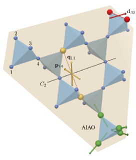
Figure 1: (Color online) The top left tetrahedron indicates the sublattice indices used in our work. The red vector in the top right tetrahedron shows the nearest-neighbor $\mathbf{d}_{32}$. The gold vectors $\mathbf{p}_{14}$ and $\mathbf{q}_{14}$ are perpendicular to the $C_{2}$ axis and span the plane in which next-nearest-neighbor $\mathbf{v}_{\langle\langle 14\rangle\rangle}$ must lie. The bottom right tetrahedron with the green vectors shows the all-in/all-out configuration.

Several important clues regarding the magnetic order have been revealed by recent muon spin resonance/relaxation and magnetization measurements on both Eu₂Ir₂O₇Zhao et al. (2011); Ishikawa et al. (2012) and Y₂Ir₂O₇Disseler et al. (2012b): in the low temperature insulating phase, these measurements suggest that localized Ir moments exhibit long-range magnetic order that may not break the pyrochlore lattice symmetry. These results are consistent with the claim that in the ground state, the Ir moments order in the non-collinear, all-in/all-out (AIAO) fashion (see Fig. 1), as was previously found in calculations for both the strong Elhajal et al. (2005) and intermediate electron correlation regimes.Wan et al. (2011); Witczak-Krempa and Kim (2012) However, the above findings cannot conclusively prove that Eu₂Ir₂O₇/Y₂Ir₂O₇ orders in the AIAO fashion; a study of the low-energy magnetic excitations is required to identify the signatures unique to the AIAO state. Indeed, recent RIXS and inelastic neutron scattering experiments have revealed the magnetic excitation spectra of other iridates such as Sr₂IrO₄Kim et al. (2012a), Sr₃Ir₂O₇Kim et al. (2012b), and Na₂IrO₃Choi et al. (2012).

In this paper, we compute the magnetic excitation spectrum in both the intermediate and strong electron correlation regimes. Starting from an effective Hubbard model in the $J_{\text{eff}}=1/2$ basis to describe Ir electrons, we study the evolution of the magnetic excitation spectrum in the intermediate-$U$ regime by computing the transverse magnetic dynamic structure factor within the random phase approximation (RPA). The robust symmetry-protected degeneracies of the spin-wave spectrum, the occurrence of Landau damping, as well as the characteristic dispersion along high symmetry directions are demonstrated to be the defining signatures of the AIAO state in the intermediate-$U$ regime. In the strong correlation limit, we derive an effective spin-model and calculate the corresponding spin-wave excitations. Through naive fitting of the RPA dynamic structure factor with the strong-coupling spin-wave results, we find that the magnetic excitation spectrum at intermediate-$U$ shows strong departures from the lowest-order spin-wave calculations. Current experiments suggest that the intermediate-coupling regime may be more suitable for describing Eu₂Ir₂O₇, where the charge gap estimated from the resistivity measurements is found to be small ($\sim 10$ meV).Zhao et al. (2011)

The rest of this paper is organized as follows. We begin with a brief description of the Hubbard model relevant to the pyrochlore iridates in Section II. We introduce a new parametrization for the tight-binding parameters, which elucidates the structure of the mean-field phase diagram presented in Section III. Subsequently, we discuss the results obtained both in the intermediate-$U$ (Section IV.1) and large-$U$ (Section IV.2) regimes. We also discuss the unique signatures of the AIAO phase and compare the results obtained in the two different regimes. Implications of our results are summarized in Section V. Further details regarding various calculations are given in the appendices.

II Microscopic Hamiltonian

In the pyrochlore iridates, $\text{Ir}^{4+}$ ions are located at the center of corner-sharing oxygen octahedra. This leads to crystal-field splitting of the $5d$ orbitals into upper $e_{g}$ and lower $t_{2g}$ orbitals. The six-fold degenerate $t_{2g}$ orbitals (including spin degeneracy) is then split into an upper $J_{\text{eff}}=1/2$ doublet and lower $J_{\text{eff}}=3/2$ quadruplet by the atomic SO coupling with energy separation of $3\lambda/2$ ($\lambda\approx 500$ meV for Ir). Therefore, in the atomic limit, the five valence electrons will fully fill the $J_{\text{eff}}=3/2$ states, half-fill the $J_{\text{eff}}=1/2$ states, and leave the $e_{g}$ orbitals unoccupied. This atomic picture suggests that the low-energy physics can be captured by considering only the half-filled $J_{\text{eff}}=1/2$ states.Kim et al. (2008, 2009) Therefore it is useful to start from the most general on-site Hubbard model in the $J_{\text{eff}}=1/2$ basis allowed by symmetry:

$$H=\sum_{ij}c_{i}^{\dagger}h_{ij}c_{j}+U\sum_{i}n_{i\uparrow}n_{i\downarrow},$$ (1)

where $i,j$ are lattice site indices, $c_{i}=(c_{i\uparrow},\>c_{i\downarrow})$ are the electron annihilation operators, $\uparrow$ and $\downarrow$ are the z-components of the psuedospin operator defined in the global basis, and $n_{i\sigma}=c^{\dagger}_{i\sigma}c_{i\sigma}$ is the electron number operator at site $i$ of psuedospin $\sigma$. In general the hopping matrix $h_{ij}$ is complex and can be constrained by considering time-reversal invariance and various space group symmetries (Moriya rules).Moriya (1960); Elhajal et al. (2005); Kurita et al. (2011)

Time-reversal invariance restricts the hopping matrix to the form:

$$h_{ij}=t_{ij}\mathbb{I}+i\mathbf{v}_{ij}\cdot\mathbf{\sigma},$$ (2)

where $\mathbb{I}$ is the $2\times 2$ identity matrix, $\mathbf{\sigma}(=\sigma_{x},\sigma_{y},\sigma_{z})$ are the Pauli matrices (in the pseudospin space), and $t_{ij}$ and $\mathbf{v}_{ij}=({\text{v}}^{x}_{ij},{\text{v}}^{y}_{ij},{\text{v}}^{z}_{ij})$ are real hopping amplitudes. Hermiticity of the Hamiltonian implies

$$t_{ij}=t_{ji}~{}~{}{\text{and}}~{}~{}\mathbf{v}_{ij}=-\mathbf{v}_{ji}.$$ (3)

$t_{ij}$ and $\mathbf{v}_{ij}$ transform as a scalar and as a psuedovector respectively under the space group symmetries of the lattice.Moriya (1960); Elhajal et al. (2005) In particular these symmetries constrain the nearest-neighbor (NN) $\mathbf{v}_{\langle ij\rangle}$s to be perpendicular to the mirror plane containing $i$ and $j$. The two possible directions that $\mathbf{v}_{\langle ij\rangle}$ can point are classified as “direct” or “indirect”.Elhajal et al. (2005) We shall denote the unit vector of the “direct” case as $\mathbf{d}_{ij}$ (see Fig. 1). For next-nearest-neighbors (NNN) $\langle\langle ij\rangle\rangle$, the two-fold rotation axis that exchanges $i$ and $j$ restricts $\mathbf{v}_{\langle\langle ij\rangle\rangle}$ to lie in the plane normal to this axis.Witczak-Krempa et al. (2012) We can parametrize this plane by the two orthonormal vectors

$$\mathbf{p}_{ij}\equiv\sqrt{6}/4\left(-\mathbf{R}_{ij}+\mathbf{D}_{ij}\right)$$ (4)

$$\mathbf{q}_{ij}\equiv\sqrt{3}/2\left(\mathbf{R}_{ij}+\mathbf{D}_{ij}\right),$$ (5)

where $\mathbf{R}_{ij}\equiv\mathbf{r}_{ik}\times\mathbf{r}_{kj}$ and $\mathbf{D}_{ij}\equiv\mathbf{d}_{ik}\times\mathbf{d}_{kj}$, site $k$ being the common NN of $i$ and $j$ (see Fig. 1).

The above constraints allow us to parametrize $h_{ij}$ by two real NN (unprimed) hopping amplitudes and three NNN (primed) hopping amplitudes:

$$h_{\langle ij\rangle}(t_{1},t_{2}) =t_{1}\mathbb{I}+it_{2}\mathbf{d}_{ij}\cdot\mathbf{\sigma},$$

$$h^{\prime}_{\langle\langle ij\rangle\rangle}(t^{\prime}_{1},t^{\prime}_{2},t^{\prime}_{3}) =t^{\prime}_{1}\mathbb{I}+i\left(t^{\prime}_{2}\mathbf{p}_{ij}+t^{\prime}_{3}\mathbf{q}_{ij}\right)\cdot\mathbf{\sigma}.$$ (6)

For the rest of the paper, instead of using $(t_{1},t_{2}),(t^{\prime}_{1},t^{\prime}_{2},t^{\prime}_{3})$ as our hopping parameters, we find it more convenient to work with $(t,\theta),(t^{\prime},\theta^{\prime},\phi^{\prime})$ which makes certain symmetries of the phase diagram readily accessible. These are defined as

$$\left(\begin{matrix}t_{1}\\ t_{2}\end{matrix}\right)=t\left(\begin{matrix}\cos(\theta_{t}/2-\theta)\\ \sin(\theta_{t}/2-\theta)\end{matrix}\right),$$ (7)

$$\left(\begin{matrix}t^{\prime}_{1}\\ t^{\prime}_{2}\\ t^{\prime}_{3}\end{matrix}\right)=t^{\prime}\left(\begin{matrix}\cos(\theta_{t}/2-\theta^{\prime})\sin(\phi^{\prime})\\ \sin(\theta_{t}/2-\theta^{\prime})\sin(\phi^{\prime})\\ \cos(\phi^{\prime})\end{matrix}\right),$$ (8)

where $\theta_{t}=2\arctan(\sqrt{2})\approx 109.47^{\circ}$ is the tetrahedral angle. This parametrization together with the definition of $\mathbf{p}_{ij}$ and $\mathbf{q}_{ij}$ naturally makes the following property of the model manifest: if we perform the basis transformation $c_{ia\alpha}\rightarrow e^{-i\pi\hat{n}_{a}\cdot\mathbf{\sigma}_{\alpha\beta}}c_{ia\beta}$, where $\hat{n}_{a}$ is the unit vector pointing from sublattice $a$ to the center of the tetrahedron, the hopping parameters $\theta$ and $\theta^{\prime}$ are transformed to $-\theta$ and $-\theta^{\prime}$ respectively. In other words, the Hamiltonian parametrized by hopping parameters $(t,\theta),(t^{\prime},\theta^{\prime},\phi^{\prime})$ yields identical features as the Hamiltonian parametrized by $(t,-\theta),(t^{\prime},-\theta^{\prime},\phi^{\prime})$.

We can also derive hopping matrices obeying the above symmetry constraints by considering the Slater-Koster approximation of orbital overlaps. In terms of this microscopic approach, the relevant Slater-Koster parameters are: (1) Ir-Ir hopping via direct overlap of $d$-orbitals. There are three such overlaps: $t_{\sigma}$ (for $\sigma$-bonds), $t_{\pi}$ (for $\pi$-bonds), and $t_{\delta}$ (for $\delta$-bonds) for NN (and primed ones for NNN), and (2) $t_{o}$ describing the hopping between the Ir atoms via the intermediate oxygen. Details of such a derivation can be found in Ref. Pesin and Balents, 2010; Witczak-Krempa and Kim, 2012; Witczak-Krempa et al., 2012 and Appendix A.

III Mean-Field Phase Diagram

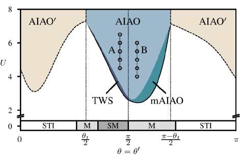
Figure 2: (Color online) Mean-field phase diagram with hopping amplitudes $\theta^{\prime}=\theta$, $t^{\prime}/t=0.1$, $t=1$, and $\phi^{\prime}=5\pi/6$. The phases in the non-interacting limit is shown at $U=0$. First order transitions are indicated by dashed lines while second order transitions are indicated by solid black lines. Lines A ($\theta=1.45$) and B ($\theta=1.70$) represent the two cuts for which the RPA dynamic structure factors are calculated (Fig. 3).

In Fig. 2, we show the mean-field phase diagram for $0<\theta<\pi$. We have chosen $\theta=\theta^{\prime}$, $t^{\prime}/t=0.1$ and $\phi^{\prime}=5\pi/6$. Throughout our calculation we have set $t=1$ as our energy scale and we comment on its possible values in physical systems in the concluding section. We note that this parametrization is somewhat different from those used in Ref. Witczak-Krempa and Kim, 2012 where the Ir-O-Ir hopping amplitude was set as the unit of energy. The phase diagram for $0>\theta>-\pi$ will be identical due to the $(t,\theta),(t^{\prime},\theta^{\prime},\phi^{\prime})\sim\!(t,-\theta),(t^{\prime},-\theta^{\prime},\phi^{\prime})$ structure as discussed in the Section II. Our phase diagram is consistent with those obtained in previous calculations.Witczak-Krempa and Kim (2012)

In the non-interacting limit, depending on the value of $\theta$, we find a strong topological-insulator (STI), the metallic (M), and the semimetallic phase (SM). The M phase has small particle- and hole-like pockets, whereas the SM phase has a quadratic-band-touching at the $\Gamma$-point at the chemical potential. At finite $U$, only two magnetic configurations are found: the all-in/all-out (AIAO) and the rotated all-in/all-out (AIAO^′) orders.Witczak-Krempa and Kim (2012) The AIAO configuration is realized by increasing $U$ starting with the SM or M phase. On the other hand, the AIAO^′ configuration is realized by increasing $U$ in the M or STI phase. Phase transitions to the AIAO^′ by an increase in $U$ is of first order. Also, the transitions between the AIAO and the AIAO^′ phases are of first order and occur at $\theta_{t}/2$ and $\pi-\theta_{t}/2$. In the non-interacting limit, band-inversion at the $\Gamma$-point also occurs at these values of $\theta$. All other transitions are of second order.

At large $U$’s, the system is gapped, while for $U$ values near the onset of magnetic order, the single-particle spectrum may continue to remain gapless even after the onset of magnetic order. The topological Weyl semimetal (TWS) and the magnetically-ordered metallic (mAIAO) phases are realized in this gapless window—the former is developed via the splitting of the quadratic-band touching at the Fermi-level of the SM phase while the latter is realized due to the presence of particle-hole pockets in the M phase.

IV Magnetic Excitation spectrum

As pointed out in Sec. III, for a sufficiently large Hubbard interaction $U$ and for $\theta_{t}/2<\theta<\pi-\theta_{t}/2$, the mean-field solution is the AIAO state. We want to study the nature of the low-energy magnetic excitation spectrum of this magnetically-ordered state, which are composed of the transverse fluctuations of the spins about their local ordering directions. We study these excitations in both the intermediate and strong electron correlation regimes and we accomplish this by applying two different and contrasting approaches. For the case of intermediate-$U$, we study the spin-waves by computing the RPA transverse spin-spin dynamic structure factor at zero temperature. In the large-$U$ regime, we perform a strong-coupling expansion of our Hubbard model (Eq. 1) to derive an effective spin-model. The spin-model is then used to calculate the spin-wave spectrum about the AIAO state within the Holstein-Primakoff approximation.

IV.1 Intermediate-$\mathbf{U}$: RPA dynamic structure factor

The information about the spin-waves are contained in the transverse part of the RPA dynamic spin-spin susceptibility matrix. This is given by:

$$\chi_{\text{RPA}\perp}(\mathbf{q},\omega)=(\mathbf{1}-U\chi_{\text{MF}\perp}(\mathbf{q},\omega))^{-1}(\chi_{\text{MF}\perp}(\mathbf{q},\omega)),$$ (9)

where $\chi_{\text{MF}\perp}$ is the bare mean-field transverse spin-spin susceptibility, and $U$ is the Hubbard repulsion. Since the pyrochlore unit cell has four sublattices, $\chi_{\text{MF}\perp}$ is a $4\times 4$ matrix. We compute the trace of the imaginary part of the RPA susceptibility, i.e., the RPA dynamic structure factor. This trace sums over the contribution of the individual spin-wave bands (there are four such bands) and gives the overall intensity that will be observed in inelastic neutron scattering or RIXS experiments. The details of the form of the susceptibility matrix is discussed in Appendix B.

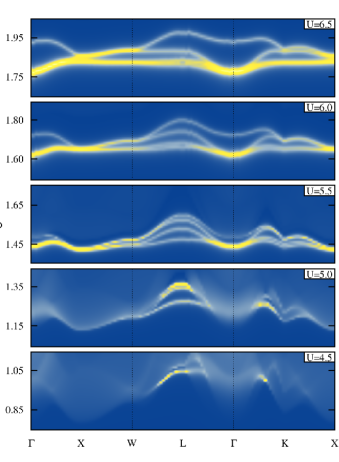
(a)

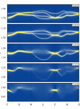
(b)

Figure 3: (Color online) RPA dynamic structure factors for (a) $\theta=1.45$ and (b) $\theta=1.70$ for various values of $U$; $\omega$ is in units of $t=1$. These correspond to cuts A and B in Fig. 2 respectively. Sharp dispersions can be seen at larger values of $U$’s, while lighter intensity and broadened spectra is seen due to Landau damping in parts of the Brillouin zone at lower $U$’s. Degeneracies at $\Gamma$, X, and W are symmetry-protected and are robust features of the AIAO state.

Results:

We consider the RPA dynamic structure factor along two representative cuts (A and B) in the phase diagram as $U$ is increased. For cut A, $\theta=1.45$ while for cut B, $\theta=1.70$ as shown in Fig. 2. Due to the presence of spin-orbit coupling ($t_{2}\neq 0$), spin-rotation symmetry is explicitly broken, and the spin-wave spectra are expected to be gapped.

The dynamic structure factors for cut A are shown in Fig. 3a. For this cut, the system is in the quadratic-band-touching SM phase in the non-interacting limit. For $U=4.5$, the low-lying particle-hole continuum damps and broadens the spin-wave spectrum throughout most of the Brillouin zone. This so-called Landau damping occurs because spin-waves decay through interactions with single-particle excitations and acquire a finite lifetime, which broadens its spectrumBuczek et al. (2011); Mohn (2003). The damping does not occur near the $L$-point, where the dispersions extend out of the continuum and produce sharp bands. As $U$ is increased, the particle-hole continuum is shifted upwards in energy throughout the Brillouin zone, revealing all four spin-wave modes. The lower energy modes are relatively dispersionless compared to the higher energy modes, which disperses most markedly near the $L$-point. At $U=6.5$, the degeneracies of the spectrum become more apparent: there are two two-fold degeneracies at the $X$- and $W$-points, while the $\Gamma$-point has a three-fold degeneracy. We note that for $U\lesssim 4.5$, which includes the TWS phase, all the spin-wave modes are damped by the particle-hole continuum.

For the second cut (Fig. 3b), the system is in the metallic phase in the non-interacting limit. Well-defined spin-wave excitations are only observed for $U\gtrsim 4.0$. Starting at $U=4.0$, the spin-wave modes appear near the $\Gamma$ point. At $U=4.5$, low-energy, damped features can be seen near the $L$-point and along the $\Gamma-K$ line. For $U=5.0$, most of the spin-wave modes become sharply defined as the particle-continuum shifts upward. As $U$ is increased further, the low-lying dispersion at $L$ shifts up and bands at $\Gamma$ begin to separate while maintaining the three-fold degeneracy required by symmetry. At $U=6.0$, the spectrum begins to resemble the $U=6.5$ spectrum of the first cut.

Degeneracies at the high symmetry points $\Gamma$, X, and W are symmetry-protected, and therefore, they are characteristic to the AIAO state, which preserves the lattice symmetry. The almost flat dispersion encountered at the zone boundary (X-W) is also a distinguishing feature.

IV.2 Strong-Coupling Expansion - Linear Spin-Wave Theory

We now look at the spin-wave spectrum in the strong-coupling limit of large $U/t$. In this limit and at half-filling, we can apply perturbation theory to obtain the following effective spin Hamiltonian at the lowest order.Pesin and Balents (2010); Witczak-Krempa and Kim (2012)

$$H_{\text{spin}} =\sum_{ij}\Lambda^{ab}_{ij}S^{a}_{i}S^{b}_{j}$$

$$=\sum_{ij}\left(J\mathbf{S}_{i}\cdot\mathbf{S}_{j}+\mathbf{D}_{ij}\cdot\mathbf{S}_{i}\times\mathbf{S}_{j}+S^{a}_{i}\Gamma^{ab}_{ij}S^{b}_{j}\right),$$ (10)

where the three terms in the last line are the trace, traceless antisymmetric, and traceless symmetric parts of $\Lambda^{ab}_{ij}$. These terms correspond to the Heisenberg, the Dzyaloshinski-Moriya (DM), and the anisotropic interactions, respectively, and are related to the hopping amplitudes of Eq. (1) by:

$$J =4U^{-1}\left(t^{2}-|\mathbf{v}|^{2}/3\right),$$

$$\mathbf{D}_{ij} =8U^{-1}t\mathbf{v}_{ij},$$

$$\Gamma^{ab}_{ij} =8U^{-1}\left({\text{v}_{ij}}^{a}{\text{v}_{ij}}^{b}-\delta^{ab}|\mathbf{v}|^{2}/3\right),$$ (11)

(the magnitude of ${\bf v}_{ij}(=|{\bf v}|)$ is site independent) which holds for both NN and NNN hopping amplitudes. The “direct” configuration of the DM vectors are known to stabilize the AIAO stateElhajal et al. (2005) which is in agreement with our earlier mean-field phase diagram. Hence we consider the low-energy spin-wave expansion about the AIAO state for the above spin Hamiltonian.

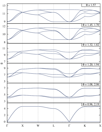
Figure 4: Evolution of the Holstein-Primakoff spin-wave spectra as angle $\theta$ is varied between $(\theta_{t}/2\approx 0.96)<\theta<(\pi-\theta_{t}/2\approx 2.19)$; $\omega$ is in units of $t^{2}/U$. $\theta$ and $\pi-\theta$ yield identical spin-wave spectra and this redundancy is reflected by each plot having two $\theta$ values. Like the RPA results in Fig. 3, degeneracies at $\Gamma$, X, and W are symmetry-protected.

To obtain the spin-wave expansion about the AIAO state which orders non-collinearly, we rotate our spin quantization axis locally in alignment with the magnetic ordering.Ross et al. (2011) To this end, we define rotated spin operators, $\tilde{\mathbf{S}}$, such that their local $S_{z}$ points to the direction of magnetic ordering at that site.

$$S^{a}_{i}=\left(\mathbf{R}_{i}(\tilde{\mathbf{S}}_{i})\right)^{a}=R^{ab}_{i}\tilde{S}^{b}_{i},$$ (12)

where $\mathbf{R}_{i}$ and $R^{ab}_{i}$ are the rotation operator and its matrix representation that takes the direction of magnetic order at site $i$ and rotates it to the z-axis of the global coordinate system. With these rotated operators, we can rewrite Eq. (IV.2):

$$H_{\text{spin}}=\sum_{ij}\left[R^{\text{T}}_{i}\Lambda_{ij}R_{j}\right]^{ab}\tilde{S}^{a}_{i}\tilde{S}^{b}_{j},$$ (13)

where $R^{\text{T}}$ indicates matrix transposition.

After recasting our spin operators in the rotated coordinate system, we are in the position to analyze the spin-waves about the AIAO state by applying linear spin-wave theory. First, we rewrite our spin operators in the Holstein-Primakoff bosonic representation:

$$\tilde{S}^{+}_{i} =\sqrt{2s-a^{\dagger}_{i}a_{i}}a_{i},$$ (14)

$$\tilde{S}^{-}_{i} =a^{\dagger}_{i}\sqrt{2s-a^{\dagger}_{i}a_{i}},$$

$$\tilde{S}^{\text{z}}_{i} =s-a^{\dagger}_{i}a_{i},$$

where $s$ is the total spin angular momentum and we have introduced four flavors of bosons, one for each sublattice of the pyrochlore unit cell. Next, we expand and truncate the spin Hamiltonian to quadratic order, Fourier transform the bosonic operators, and solve for the resulting excitation spectrum via a Bogoliubov transformation.

Results:

We consider the spin-wave spectra obtained from the effective spin Hamiltonian generated by only NN hopping amplitudes. Adding up to $t^{\prime}=0.1~{}t$ NNN hopping amplitudes (not shown) only leads to small changes (see below). In Fig. 4, we depict the evolution of the spin-wave spectrum as the NN hopping parameter $\theta$ is varied. In the absence of NNN hopping amplitudes, $\theta$ and $\pi-\theta$ yield identical spin-wave spectra. This structure is again related to our choice of angular parametrization: $\theta$ and $-\theta$ are related by a basis transformation and should therefore have the same spin-wave spectrum. Moreover, $-\theta\rightarrow-\theta+\pi$ is equivalent to $t\rightarrow-t$ and $\mathbf{v}\rightarrow-\mathbf{v}$, which leaves $J$, $\mathbf{D}_{ij}$, and $\Gamma_{ij}$ invariant. Hence, $\theta$ and $\pi-\theta$ yield the same spin-wave spectrum and this fact is noted by assigning each of the plots in Fig. 4 with two $\theta$ values.

For $\theta_{t}/2<\theta<\pi-\theta_{t}/2$, the spin-wave spectrum is gapped and the gap decreases as we approach either endpoints of the interval. At the endpoints, two of the four bands of the spectrum become both gapless and dispersionless, while outside the endpoints, the lowest bands become negative in energy, signaling an instability of the AIAO state. The onset of these instabilities is consistent with NN mean-field theory results, which predicts first order transitions (between the AIAO to the AIAO^′ phase) at $\theta=\theta_{t}/2$ and $\theta=\pi-\theta_{t}/2$.

We note that the degeneracies at the high-symmetry points $\Gamma$, X, and W are consistent with the RPA results as they are protected by symmetry. Also, the flat dispersions at the zone boundary (X-W) is also encountered in the present spin-wave calculation. On the other hand, the lowest energy dispersion along the L-$\Gamma$ line is absolutely flat in this NN model. However, on adding small NNN hopping (up to $t^{\prime}=0.1~{}t$), it acquires small dispersion. This should be contrasted with RPA results in Fig. 3 where modes along the L-$\Gamma$ line are more strongly dispersive.

IV.3 Comparison of RPA and strong-coupling results

As the ratio of typical hopping scale to the Hubbard repulsion scale ($t/U$) increases, the higher-order contributions to the strong-coupling perturbative expansion (in $t/U$) become increasingly important and the strictly NN model we employed in Section IV.2 becomes inadequate in describing the magnetic excitations of the AIAO state. Not only do higher-order contributions generate further-neighbor Heisenberg exchanges, ring-exchange type terms arise and lead to renormalization of NN quadratic terms at the linear spin-wave level.Chernyshev et al. (2004); Delannoy et al. (2005) Therefore, we should not expect a perfect agreement between the RPA and strong-coupling results.

Nevertheless, we attempt to fit (by eye estimation) the RPA results for large $U$ (e.g., $U=6.0$ in cut B) with a linear spin-wave (LSW) spectrum. First, we fit the RPA dispersion features and overall bandwidth, resulting in $J=0.13$, $|\mathbf{D}|=0.13$, $|\Gamma|=0.07$ (see Eq. IV.2 for definitions). These parameter values are different from those obtained from Eq. IV.2 which is based strictly on the leading order strong-coupling expansion for the NNs. The gap obtained from the RPA calculation is $\Delta_{\text{RPA}}\approx 1.70$.

The resulting LSW fit captures the dispersion along $\Gamma$-X-W quite well, but fails to capture the low-lying modes along the L-$\Gamma$ line and, in general, the higher energy modes where the fit at best is qualitative. We would also like to point out that fits at lower $U$ and along cut A have been attempted but large discrepancies in both the features of the spectrum and the spin-wave gap have been found.

The above fitting results points out that the NN spin-model (and also the NNN spin-model with up to $10\%$ NNN hopping amplitude) is grossly inadequate to fit the RPA spin-wave spectrum quantitatively for parameter values that encompasses the regime appropriate for the pyrochlore iridates. In this context we would like to point out that recent estimates of small charge gap ($\sim\!10$ meV) from the resistivity measurements in Eu₂Ir₂O₇ Zhao et al. (2011); Ishikawa et al. (2012) seems to suggest that the intermediate-coupling calculations may be better suited to describe this compound.

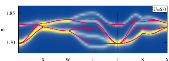
Figure 5: (Color online) RPA results at $U=6.0$ for cut B (blue and yellow color-map) overlaid with a fit with the NN linear spin-wave spectrum (red); $\omega$ is in units of $t=1$. Though some features along the $\Gamma$-X-W line can be fitted, other high-symmetry lines show a larger discrepancy.

V Summary

To summarize, we have calculated the structure of the magnetic excitation spectrum for the AIAO state that has been proposed for the pyrochlore iridates such as Eu₂Ir₂O₇ or Y₂Ir₂O₇. For intermediate correlations, we have calculated the transverse spin-spin dynamic structure factor within the RPA approximation. Features particular to the AIAO configuration that can lead to conclusive identification of the magnetic order in Eu₂Ir₂O₇ and Y₂Ir₂O₇ were discussed. For the large-$U$ limit, we used a strong-coupling expansion to derive a spin-model and calculated the linear spin-wave spectrum using the Holstein-Primakoff approximation. By fitting the RPA results with the linear spin-wave spectrum, we showed that results in the intermediate correlation regime are substantially different from those obtained from the strong-coupling theory.

Finally, from our calculations, we can make rough estimates of the experimental energy scales for the excitation gap and dispersion bandwidth by using Slater-Koster parametrization of orbital overlaps (the relation connecting the symmetry-allowed parameters in Eq. II to Slater-Koster parameters are detailed in Appendix A). Similar to Refs. Witczak-Krempa and Kim, 2012; Witczak-Krempa et al., 2012, we have used $t_{\pi}=-2t_{\sigma}/3$, $t_{\delta}=0$, while $t_{\sigma}=-1.16t_{o}(-1.37t_{o})$ for cut $A(B)$ (the different orbital overlaps were introduced towards the end of Section II and are also used in Appendix A). Typically, the value of $t_{o}$—the Ir-O-Ir hopping—is about $200$–$350$ meV in iridates with octahedral oxygen environments.Norman and Micklitz (2010); Kim et al. (2012c) Here we choose a representative value of $t_{o}\approx 300$ meV. With these values, in Fig. 3, the spin gap found from our RPA calculation is on the order of $100$ meV and the dispersion width is on the order of $\sim\!15$ meV. This value of spin gap is found to be very sensitive to the value of $U$ while the bandwidth always remains in the same regime. While a $100$ meV gap can be resolved within current RIXS resolution, the dispersion width may be presently on the borderline of resolvability.

In other iridium compounds, recent progress have been made in RIXSKim et al. (2012a, b); Gretarsson et al. (2012), neutron scatteringChoi et al. (2012); Ye et al. (2012), resonant magnetic x-ray scattering (RMXS)Liu et al. (2011); Clancy et al. (2012a), and x-ray absorption spectroscopy (XAS)Clancy et al. (2012b) experiments. In particular, RIXS and inelastic neutron scattering experiments have recently revealed the magnetic excitation spectra of Sr₂IrO₄Kim et al. (2012a), Sr₃Ir₂O₇Kim et al. (2012b), and Na₂IrO₃Choi et al. (2012). Future applications of these techniques and improvements in experimental resolution may help reveal the magnetic behavior and, in particular, the magnetic excitation spectra of pyrochlore iridates, thereby conclusively determining the nature of their magnetic order.

Appendix A Microscopic origins of hopping parameters

In order to estimate the values of the hopping parameters, we turn to a microscopic analysis of hopping paths. We briefly discuss the results of such an analysis and refer to Ref. Yang and Kim, 2010; Pesin and Balents, 2010; Witczak-Krempa et al., 2012 for more details.

We consider two types of hopping: Ir-Ir hopping via overlap of $d$-orbitals and O-Ir hopping between $p$-orbitals of O and $d$-orbitals of Ir. We parametrize $d$-$d$ overlaps with Slater-Koster amplitudes $t_{\sigma}$, $t_{\pi}$, and $t_{\delta}$ (and primed ones for NNN), while for $p$-$d$ overlaps, we parametrize them with amplitudes $t_{pd\sigma}$, $t_{pd\pi}$, and O-Ir occupation energy difference $\epsilon$. Here the subscripts $\sigma,\pi$ and $\delta$ denotes the type of overlap of the orbitals. Also, in this microscopic picture, we always work in the local axes defined by the oxygen octahedra surrounding each Ir.

To arrive at a $J_{\text{eff}}=1/2$ model, we first employ second order perturbation on the O-Ir hopping to generate an effective NN Ir-Ir hopping between $d$-orbitals. This indirect hopping is given by

$$t_{\text{o}}=t^{2}_{pd\pi}/|\epsilon|$$ (15)

where $\epsilon$ is the difference of the on-site charging energies between the oxygen $2$p orbitals and Ir $5$d orbitals. (This indirect hopping receives contribution from the $t_{pd\sigma}$ overlap in presence of distortion in the oxygen octahedra). We now project the $d$-orbitals into the local $t_{2g}$ and, finally, into the local $J_{\text{eff}}=1/2$ basis, to find the hopping matrix which has the form given by Eq. (II), where the relation with the effective hopping parameters and more microscopic Slater-Koster parameters is given by the following relations

$$t_{1} =\frac{1}{972}\left(51t_{\sigma}-316t_{\pi}-43t_{\delta}+520t_{\text{o}}\right),$$

$$t_{2} =\frac{\sqrt{2}}{972}\left(60t_{\sigma}-160t_{\pi}-220t_{\delta}+112t_{\text{o}}\right),$$

$$t^{\prime}_{1} =\frac{1}{8748}\left(699t^{\prime}_{\sigma}-1628t^{\prime}_{\pi}-1843t^{\prime}_{\delta}\right),$$

$$t^{\prime}_{2} =\frac{\sqrt{2}}{8748}\left(-156t^{\prime}_{\sigma}-2720t^{\prime}_{\pi}-4t^{\prime}_{\delta}\right),$$

$$t^{\prime}_{3} =\frac{1}{8748}\left(-144t^{\prime}_{\sigma}-960t^{\prime}_{\pi}+1104t^{\prime}_{\delta}\right),$$ (16)

From these relations, it is straightforward to use Eqs. 7 and 8 to relate the angular parameters to the above Slater-Koster parameters.

The range of physical NN hopping parameters explored in Ref. Witczak-Krempa et al., 2012 ($-1.2\lesssim t_{\sigma}\lesssim-0.5$, $t_{\pi}=-2t_{\sigma}/3$, $t_{\delta}=0$ and $t_{o}=1$) corresponds to $0.85\lesssim\theta\lesssim 1.51$ with the appropriate energy scaling of $t$.

Appendix B Mean-field transverse spin-spin susceptibility

As Eq. 9 indicates, we need to compute the mean-field transverse spin-spin susceptibility in order to obtain the RPA susceptibility. Here we provide details of such calculation for non-collinear magnetic order like the AIAO state.

The mean-field susceptibility matrix is given by:

$$\mathcal{\chi}^{ab}_{\text{MF}\perp}(\mathbf{q},t)=-i\Theta(t)\left\langle\left[(\mathbf{S}^{a}_{\perp}(\mathbf{q},t))_{i},(\mathbf{S}^{b}_{\perp}(-\mathbf{q},0))_{i}\right]\right\rangle,$$ (17)

where $\mathbf{S}^{a}_{\perp}(\mathbf{q},t)$ denotes the Fourier transform of the component of the spin operator that is perpendicular to the magnetic ordering direction for sublattice $a$ (see Fig. 1 for sublattice convention), and $i$ indexes the components of $\mathbf{S}^{a}_{\perp}(\mathbf{q},t)$, which are to be summed over. If the direction of magnetic moment on sublattice is given by the unit vector $\hat{n}^{a}$, then the transverse spin operator for that sublattice is given by

$$\mathbf{S}^{a}_{\perp}(\mathbf{q})=-\hat{n}^{a}\times(\hat{n}^{a}\times\mathbf{S}^{a}(\mathbf{q})),$$ (18)

where $\mathbf{S}^{a}(\mathbf{q})$ is the Fourier transform of the spin operator. For the AIAO state, $\hat{n}^{a}$ points along the local [111] direction of the lattice.

We write the spin operator with electron operators as

$$\mathbf{S}^{a}(\mathbf{q})=\frac{1}{2}\sum_{\bf k}c^{\dagger}_{{\bf k}+{\bf q},\alpha}\bm{\sigma}_{\alpha\beta}c_{{\bf k},\beta}$$ (19)

where $\alpha,\beta=\uparrow,\downarrow$. Using this we get

$$\mathcal{\chi}^{ab}_{\text{MF}\perp}(\mathbf{q},t)=-iM^{ab}_{\alpha\beta\gamma\delta}\Theta(t)$$ (20)

$$\times\sum_{\mathbf{k}_{1}\mathbf{k}_{2}}\left\langle\left[c_{a\alpha}^{\dagger}(\mathbf{q}+\mathbf{k}_{1},t)c_{a\beta}(q_{1},t),c_{b\gamma}^{\dagger}(-\mathbf{q}+\mathbf{k}_{2},0)c_{b\delta}(\mathbf{k}_{2},0)\right]\right\rangle,$$

with

$$M^{ab}_{\alpha\beta\gamma\delta} =\frac{1}{2}\left(\hat{n}^{a}\times\left(\hat{n}^{a}\times\mathbf{\sigma}_{\alpha\beta}\right)\right)\cdot\frac{1}{2}\left(\hat{n}^{b}\times\left(\hat{n}^{b}\times\mathbf{\sigma}_{\gamma\delta}\right)\right),$$ (21)

Lastly, we transform our basis to the band basis using the results from our Hartree-Fock mean-field calculation, evaluate the two-body expectation value via Wick’s theorem, and Fourier transform to frequency space to obtain $\mathcal{\chi}^{ab}_{\text{MF}\perp}(\mathbf{q},\omega)$.

References

- Machida et al. (2010) Y. Machida, S. Nakatsuji, S. Onoda, T. Tayama, and T. Sakakibara, Nature 463, 210 (2010).
- Machida et al. (2007) Y. Machida, S. Nakatsuji, Y. Maeno, T. Tayama, T. Sakakibara, and S. Onoda, Phys. Rev. Lett. 98, 057203 (2007).
- Witczak-Krempa and Kim (2012) W. Witczak-Krempa and Y. B. Kim, Phys. Rev. B 85, 045124 (2012).
- Go et al. (2012) A. Go, W. Witczak-Krempa, G. S. Jeon, K. Park, and Y. B. Kim, Phys. Rev. Lett. 109, 066401 (2012).
- Yang and Kim (2010) B.-J. Yang and Y. B. Kim, Phys. Rev. B 82, 085111 (2010).
- Pesin and Balents (2010) D. Pesin and L. Balents, Nature Physics 6, 376 (2010).
- Wan et al. (2011) X. Wan, A. M. Turner, A. Vishwanath, and S. Y. Savrasov, Phys. Rev. B 83, 205101 (2011).
- Kim et al. (2008) B. J. Kim, H. Jin, S. J. Moon, J.-Y. Kim, B.-G. Park, C. S. Leem, J. Yu, T. W. Noh, C. Kim, S.-J. Oh, J.-H. Park, V. Durairaj, G. Cao, and E. Rotenberg, Phys. Rev. Lett. 101, 076402 (2008).
- Kim et al. (2009) B. J. Kim, H. Ohsumi, T. Komesu, S. Sakai, T. Morita, H. Takagi, and T. Arima, Science 323, 1329 (2009).
- Matsuhira et al. (2011) K. Matsuhira, M. Wakeshima, Y. Hinatsu, and S. Takagi, Journal of the Physical Society of Japan 80, 094701 (2011).
- Zhao et al. (2011) S. Zhao, J. M. Mackie, D. E. MacLaughlin, O. O. Bernal, J. J. Ishikawa, Y. Ohta, and S. Nakatsuji, Phys. Rev. B 83, 180402 (2011).
- Fukazawa and Maeno (2002) H. Fukazawa and Y. Maeno, Journal of the Physical Society of Japan 71, 2578 (2002).
- Aito et al. (2003) N. Aito, M. Soda, Y. Kobayashi, and M. Sato, Journal of the Physical Society of Japan 72, 1226 (2003).
- Nakatsuji et al. (2006) S. Nakatsuji, Y. Machida, Y. Maeno, T. Tayama, T. Sakakibara, J. v. Duijn, L. Balicas, J. N. Millican, R. T. Macaluso, and J. Y. Chan, Phys. Rev. Lett. 96, 087204 (2006).
- Kargarian et al. (2011) M. Kargarian, J. Wen, and G. A. Fiete, Phys. Rev. B 83, 165112 (2011).
- Singh et al. (2008) R. S. Singh, V. R. R. Medicherla, K. Maiti, and E. V. Sampathkumaran, Phys. Rev. B 77, 201102 (2008).
- Kurita et al. (2011) M. Kurita, Y. Yamaji, and M. Imada, Journal of the Physical Society of Japan 80, 044708 (2011).
- Disseler et al. (2012a) S. M. Disseler, C. Dhital, T. C. Hogan, A. Amato, S. R. Giblin, C. de la Cruz, A. Daoud-Aladine, S. D. Wilson, and M. J. Graf, Phys. Rev. B 85, 174441 (2012a).
- Disseler et al. (2012b) S. M. Disseler, C. Dhital, A. Amato, S. R. Giblin, C. de la Cruz, S. D. Wilson, and M. J. Graf, Phys. Rev. B 86, 014428 (2012b).
- Tafti et al. (2012) F. F. Tafti, J. J. Ishikawa, A. McCollam, S. Nakatsuji, and S. R. Julian, Phys. Rev. B 85, 205104 (2012).
- Chen and Hermele (2012) G. Chen and M. Hermele, (2012), arXiv:1208.4853 [cond-mat.str-el] .
- Yanagishima and Maeno (2001) D. Yanagishima and Y. Maeno, Journal of the Physical Society of Japan 70, 2880 (2001).
- Taira et al. (2001) N. Taira, M. Wakeshima, and Y. Hinatsu, Journal of Physics: Condensed Matter 13, 5527 (2001).
- Matsuhira et al. (2007) K. Matsuhira, M. Wakeshima, R. Nakanishi, T. Yamada, A. Nakamura, W. Kawano, S. Takagi, and Y. Hinatsu, Journal of the Physical Society of Japan 76, 043706 (2007).
- Ishikawa et al. (2012) J. J. Ishikawa, E. C. T. O’Farrell, and S. Nakatsuji, Phys. Rev. B 85, 245109 (2012).
- Tomiyasu et al. (2012) K. Tomiyasu, K. Matsuhira, K. Iwasa, M. Watahiki, S. Takagi, M. Wakeshima, Y. Hinatsu, M. Yokoyama, K. Ohoyama, and K. Yamada, Journal of the Physical Society of Japan 81, 034709 (2012).
- Sakata et al. (2011) M. Sakata, T. Kagayama, K. Shimizu, K. Matsuhira, S. Takagi, M. Wakeshima, and Y. Hinatsu, Phys. Rev. B 83, 041102 (2011).
- Shapiro et al. (2012) M. C. Shapiro, S. C. Riggs, M. B. Stone, C. R. de la Cruz, S. Chi, A. A. Podlesnyak, and I. R. Fisher, Phys. Rev. B 85, 214434 (2012).
- Elhajal et al. (2005) M. Elhajal, B. Canals, R. Sunyer, and C. Lacroix, Phys. Rev. B 71, 094420 (2005).
- Kim et al. (2012a) J. Kim, D. Casa, M. H. Upton, T. Gog, Y.-J. Kim, J. F. Mitchell, M. van Veenendaal, M. Daghofer, J. van den Brink, G. Khaliullin, and B. J. Kim, Phys. Rev. Lett. 108, 177003 (2012a).
- Kim et al. (2012b) J. Kim, A. H. Said, D. Casa, M. H. Upton, T. Gog, M. Daghofer, G. Jackeli, J. van den Brink, G. Khaliullin, and B. J. Kim, Phys. Rev. Lett. 109, 157402 (2012b).
- Choi et al. (2012) S. K. Choi, R. Coldea, A. N. Kolmogorov, T. Lancaster, I. I. Mazin, S. J. Blundell, P. G. Radaelli, Y. Singh, P. Gegenwart, K. R. Choi, S.-W. Cheong, P. J. Baker, C. Stock, and J. Taylor, Phys. Rev. Lett. 108, 127204 (2012).
- Moriya (1960) T. Moriya, Phys. Rev. 120, 91 (1960).
- Witczak-Krempa et al. (2012) W. Witczak-Krempa, A. Go, and Y. B. Kim, (2012), arXiv:1208.4099 [cond-mat.str-el] .
- Buczek et al. (2011) P. Buczek, A. Ernst, and L. M. Sandratskii, Phys. Rev. B 84, 174418 (2011).
- Mohn (2003) P. Mohn, Magnetism in the solid state : an introduction (Springer, New York, 2003).
- Ross et al. (2011) K. A. Ross, L. Savary, B. D. Gaulin, and L. Balents, Phys. Rev. X 1, 021002 (2011).
- Chernyshev et al. (2004) A. L. Chernyshev, D. Galanakis, P. Phillips, A. V. Rozhkov, and A.-M. S. Tremblay, Phys. Rev. B 70, 235111 (2004).
- Delannoy et al. (2005) J.-Y. P. Delannoy, M. J. P. Gingras, P. C. W. Holdsworth, and A.-M. S. Tremblay, Phys. Rev. B 72, 115114 (2005).
- Norman and Micklitz (2010) M. R. Norman and T. Micklitz, Phys. Rev. B 81, 024428 (2010).
- Kim et al. (2012c) C. H. Kim, H. S. Kim, H. Jeong, H. Jin, and J. Yu, Phys. Rev. Lett. 108, 106401 (2012c).
- Gretarsson et al. (2012) H. Gretarsson, J. P. Clancy, X. Liu, J. P. Hill, E. Bozin, Y. Singh, S. Manni, P. Gegenwart, J. Kim, A. H. Said, D. Casa, T. Gog, M. H. Upton, H.-S. Kim, J. Yu, V. M. Katukuri, L. Hozoi, J. van den Brink, and Y.-J. Kim, (2012), arXiv:1209.5424 [cond-mat.str-el] .
- Ye et al. (2012) F. Ye, S. Chi, H. Cao, B. C. Chakoumakos, J. A. Fernandez-Baca, R. Custelcean, T. F. Qi, O. B. Korneta, and G. Cao, Phys. Rev. B 85, 180403 (2012).
- Liu et al. (2011) X. Liu, T. Berlijn, W.-G. Yin, W. Ku, A. Tsvelik, Y.-J. Kim, H. Gretarsson, Y. Singh, P. Gegenwart, and J. P. Hill, Phys. Rev. B 83, 220403 (2011).
- Clancy et al. (2012a) J. P. Clancy, K. W. Plumb, C. S. Nelson, Z. Islam, G. Cao, T. Qi, and Y.-J. Kim, (2012a), arXiv:1207.0960 [cond-mat.str-el] .
- Clancy et al. (2012b) J. P. Clancy, N. Chen, C. Y. Kim, K. W. Plumb, B. C. Jeon, T. W. Noh, and Y.-J. Kim, (2012b), arXiv:1205.6540 [cond-mat.str-el] .
- Loken et al. (2010) C. Loken, D. Gruner, L. Groer, R. Peltier, N. Bunn, M. Craig, T. Henriques, J. Dempsey, C.-H. Yu, J. Chen, L. J. Dursi, J. Chong, S. Northrup, J. Pinto, N. Knecht, and R. V. Zon, Journal of Physics: Conference Series 256, 012026 (2010).