On diffusion in narrow random channels

Abstract

We consider in this paper a solvable model for the motion of molecular motors. Based on the averaging principle, we reduce the problem to a diffusion process on a graph. We then calculate the effective speed of transportation of these motors.

Keywords: Brownian motors/ratchets, averaging principle, diffusion processes on graphs, random environment.

2010 Mathematics Subject Classification Numbers: 60H30, 60J60, 92B05, 60K37.

1 Introduction

One of the possible ways to model Brownian motors/ratchets is to describe them as particles (which model the protein molecules) traveling along a designated track (see [7]). At a microscopic scale such a motion is conveniently described as a diffusion process with a deterministic drift. On the other hand, the designated track along which the molecule is traveling can be viewed as a tubular domain of some random shape. In particular, such a domain can have many random ”wings” added to it. (See Fig.1. The shaded areas represent the ”wings”.) In this paper we are going to introduce a mathematically solvable model of the Brownian motor and discuss some interesting relevant questions around this problem. Our model is based on ideas similar to that of [5] and [2, Chapter 7].

The model is as follows. Let $h_{0}^{\pm}(x)$ be a pair of piecewise smooth functions with $h_{0}^{+}(x)-h_{0}^{-}(x)=l_{0}(x)>0$. Let $D_{0}=\{(x,z):x\in\mathbb{R},h_{0}^{-}(x)\leq z\leq h_{0}^{+}(x)\}$ be a tubular $2$-d domain of infinite length, i.e. it goes along the whole $x$-axis. At the discontinuities of $h_{0}^{\pm}(x)$, we connect the pieces of the boundary via straight vertical lines. The domain $D_{0}$ models the ”main” channel in which the motor is traveling. Let a sequence of ”wings” $D_{j}$ ($j\geq 1$) be attached to $D_{0}$. These wings are attached to $D_{0}$ at the discontinuities of the functions $h_{0}^{\pm}(x)$.

Consider the union $D=D_{0}\bigcup\left(\bigcup\limits_{j=1}^{\infty}D_{j}\right)$. An example of such a domain $D$ is shown in Fig.1, in which one can see four ”wings” $D_{1},D_{2},D_{3},D_{4}$. We assume that, after adding the ”wings”, for the domain $D$, the boundary $\partial D$ has two smooth pieces: the upper boundary and the lower boundary. Let $\boldsymbol{n}(x,z)=(n_{1}(x,z),n_{2}(x,z))$ be the inward unit normal vector to $\partial D$. We make some assumptions on the domain $D$.

Assumption 1. The set of points $x\in\mathbb{R}$ for which there are points $(x,z)\in\partial D$ at which the unit normal vector $\boldsymbol{n}(x,z)$ is parallel to the $x$-axis: $n_{2}(x,z)=0$ has no limit points in $\mathbb{R}$. Each such point $x$ corresponds to only one point $(x,z)\in\partial D$ for which $n_{2}(x,z)=0$.

Assumption 2. For every $x$ the cross-section of the region $D$ at level $x$, i.e., the set of all points belonging to $D$ with the first coordinate equal to $x$, consists of either one or two intervals that are its connected components. That is to say, in the case of one interval this interval corresponds to the ”main channel” $D_{0}$; and in the case of two intervals one of them corresponds to the ”main channel” $D_{0}$ and the other one corresponds to the wing. The wing will not have additional branching structure. Also, for some $0<l_{0}<\bar{l}_{0}<\infty$ we have $\l_{0}\leq h_{0}^{+}(x)-h_{0}^{-}(x)=l_{0}(x)\leq\bar{l}_{0}$.

Let us take into account randomness of the domain $D$. Keeping the above assumptions in mind, we can assume that the functions $h_{0}^{\pm}(x)$ and the shape of the wings $D_{k}$ ($k=1,2,...$) are all random. Thus we can view the shape of $D$ as random. We introduce a filtration $\mathcal{F}_{s}^{t}$, $-\infty\leq s<t\leq\infty$ as the smallest $\sigma$-algebra corresponding to the shape of $D\cap\{(x,z):x\in[s,t]\}$. We introduce stationarity and mixing assumptions. Let us consider some $A\in\mathcal{F}_{s}^{t}$, $-\infty\leq s<t\leq\infty$. The set $A$ consists of some shapes of the domain $D\cap\{(x,z):x\in[s,t]\}$. Let $\theta_{r}$ ($r\in\mathbb{R}$) be the operator corresponding to the shift along $x$-direction: $\theta_{r}(A)\in\mathcal{F}_{s+r}^{t+r}$ consists of the same shapes as those in $A$ but correspond to the domain $D\cap\{(x,z):x\in[s+r,t+r]\}$.

Assumption 3. (stationarity) We have $\mathbf{P}(A)=\mathbf{P}(\theta_{r}(A))$.

Assumption 4. (mixing) For any $A\in\mathcal{F}_{s}^{t}$ and any $B\in\mathcal{F}_{s+r}^{t+r}$ we have

$$\lim\limits_{r\rightarrow\pm\infty}|\mathbf{P}(A\cap B)-\mathbf{P}(A)\mathbf{P}(B)|=0$$

exponentially fast.

For instance, we can assume that there exists some $M>0$ such that $\mathbf{P}(A\cap B)=\mathbf{P}(A)\mathbf{P}(B)$ for $|r|\geq M$.

Here and below the symbols $\mathbf{P}$ and $\mathbf{E}$ etc. refer to probabilities and expectations etc. with respect to the filtration $\{\mathcal{F}_{s}^{t}\}_{-\infty\leq s<t\leq\infty}$.

In many problems it is natural to assume that the domain $D$ is a thin and long channel. This leads to the formulation of the problem as follows. Let $D^{\varepsilon}=\{(x,\varepsilon z):(x,z)\in D\}$. The parameter $\varepsilon>0$ is small. Consider the diffusion process $\widehat{\boldsymbol{X}}_{t}^{\varepsilon}=(\widehat{X}_{t}^{\varepsilon},\widehat{Z}_{t}^{\varepsilon})$ in the domain $D^{\varepsilon}$, which is described by the following system of stochastic differential equations:

$$\left\{\begin{array}[]{l}d\widehat{X}_{t}^{\varepsilon}=dW_{t}^{1}+V(\widehat{X}_{t}^{\varepsilon},\widehat{Z}_{t}^{\varepsilon}/\varepsilon)dt+\nu_{1}(\widehat{X}_{t}^{\varepsilon},\widehat{Z}_{t}^{\varepsilon})d\widehat{\ell}_{t}^{\varepsilon}\ ,\\ d\widehat{Z}_{t}^{\varepsilon}=dW_{t}^{2}+\nu_{2}(\widehat{X}_{t}^{\varepsilon},\widehat{Z}_{t}^{\varepsilon})d\widehat{\ell}_{t}^{\varepsilon}\ .\end{array}\right.$$

Here the scalar field $V(x,z)>0,(x,z)\in D$ characterizes the speed of the transportation in the $x$-direction. The vector field $\boldsymbol{\nu}=(\nu_{1},\nu_{2})$ on $\partial D^{\varepsilon}$ is defined as the inward unit normal vector at the corresponding point on $\partial D$: $\boldsymbol{\nu}(x,\varepsilon z)=\boldsymbol{n}(x,z)$ when $(x,z)\in\partial D$. The process $(W_{t}^{1},W_{t}^{2})$ is a standard $2$-dimensional Wiener process. We make another assumption here.

Assumption 5. The process $(W_{t}^{1},W_{t}^{2})$ is independent of the filtration $\{\mathcal{F}_{s}^{t}\}_{-\infty\leq s<t\leq\infty}$ corresponding to the shape of $D$.

In other words our process $\widehat{\boldsymbol{X}}_{t}^{\varepsilon}$ is moving in an independent random environment characterized by random shape of the domain $D$.

The process $\widehat{\ell}_{t}^{\varepsilon}$ is the local time of the process $\widehat{\boldsymbol{X}}_{t}^{\varepsilon}$ at $\partial D^{\varepsilon}$.

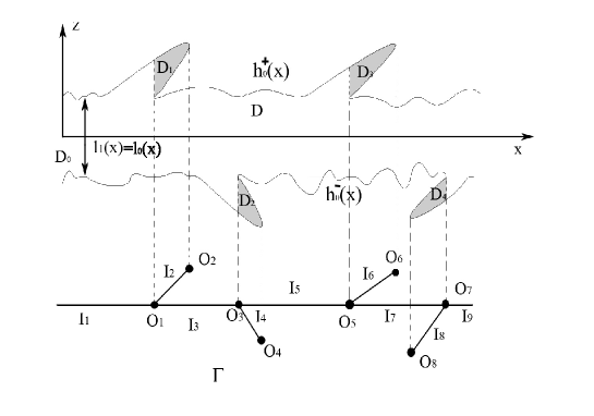
Fig. 1: A model of the molecular motor.

Making a change of variable $\widehat{Z}_{t}^{\varepsilon}\rightarrow\widehat{Z}_{t}^{\varepsilon}/\varepsilon=Z_{t}^{\varepsilon}$ in the equation (1), we can equivalently consider the diffusion process $\boldsymbol{X}_{t}^{\varepsilon}=(X_{t}^{\varepsilon},Z_{t}^{\varepsilon})$ in the original domain $D$ as follows:

$$\left\{\begin{array}[]{l}dX_{t}^{\varepsilon}=dW_{t}^{1}+V(X_{t}^{\varepsilon},Z_{t}^{\varepsilon})dt+\nu_{1}^{\varepsilon}(X_{t}^{\varepsilon},Z_{t}^{\varepsilon})d\ell_{t}^{\varepsilon}\ ,\\ dZ_{t}^{\varepsilon}=\dfrac{1}{\varepsilon}dW_{t}^{2}+\nu_{2}^{\varepsilon}(X_{t}^{\varepsilon},Z_{t}^{\varepsilon})d\ell_{t}^{\varepsilon}\ ,\end{array}\right.$$

Here $\boldsymbol{\nu}^{\varepsilon}$ is the co-normal vector field corresponding to the operator $\dfrac{1}{2\varepsilon^{2}}\dfrac{\partial^{2}}{\partial z^{2}}+\dfrac{1}{2}\dfrac{\partial^{2}}{\partial x^{2}}$: $\boldsymbol{\nu}^{\varepsilon}(x,z)=(\nu^{\varepsilon}_{1}(x,z),\nu^{\varepsilon}_{2}(x,z))\equiv(\varepsilon n_{1}(x,z),n_{2}(x,z))$. The process $\ell_{t}^{\varepsilon}$ is the local time of the process $\boldsymbol{X}_{t}^{\varepsilon}$ at $\partial D$.

Here and below we use the symbols $\mathbf{P}^{W}$ and $\mathbf{E}^{W}$ etc. (sometimes with a subscript to denote the starting point of the process) to refer to probabilities and expectations etc. with respect to the filtration generated by the 2-d Wiener process $(W_{t}^{1},W_{t}^{2})$.

The process $\boldsymbol{X}_{t}^{\varepsilon}$ has the ”fast” and the ”slow” components. The ”fast” component is the process $Z_{t}^{\varepsilon}$ and the ”slow” component is the process $X_{t}^{\varepsilon}$. According to the averaging principle we can expect a mixing in the ”fast” component before the ”slow” component $X_{t}^{\varepsilon}$ changes significantly. We shall describe the limiting slow motion.

In the next section we will characterize the limiting slow motion, which is a diffusion process on a graph. This graph corresponds to the domain $D$. A sketch of the proof of this result is in Section 3.

An interesting question arising in the applications is to calculate the effective speed of the particles. In mathematical language this problem can be formulated as follows. Let $\sigma^{\varepsilon}((-\infty,a])$ be the first time that the process $\boldsymbol{X}_{t}^{\varepsilon}$, starting from a point $\boldsymbol{x}_{0}=(x_{0},z_{0})\in D$, hits $D\cap\{x=a>0\}$. The limit

$$\lim\limits_{a\rightarrow\infty}\lim\limits_{\varepsilon\downarrow 0}\dfrac{\sigma^{\varepsilon}((-\infty,a])}{a}$$

exists in $\mathbf{P}\times\mathbf{P}^{W}_{(x_{0},z_{0})}$-probability and can be viewed as the inverse of the average effective speed of transportation of the particle inside $D$. Using the results in Sections 2 and 3 we can calculate this limit. This is done in Section 4. (In particular, see Theorem 7.)

In the last Section 5 we mention briefly problems for multidimensional channels, for random channels changing in time, and some other generalizations.

2 The limiting process

Let us, for the present and for the next section, work with a fixed shape of $D$. In the language of random motions in random environment the convergence results that we are going to state are in the so called ”quenched” setting. We will allow this shape to be random in Section 4. We shall find the limiting slow motion of the diffusion process $\boldsymbol{X}_{t}^{\varepsilon}$ inside $D$.

First of all we need to construct from the domain $D$ a graph $\Gamma$ (see Fig.1). For $x_{0}\in\mathbb{R}$ let $C(x_{0})=\{(x,z)\in D:x=x_{0}\}$ be the cross-section of the domain $D$ with the line $\{x=x_{0}\}$. The set $C(x_{0})$ may have several connected components. We identify all points in each connected component and the set thus obtained, equipped with the natural topology, is homeomorphic to a graph $\Gamma$. We label the edges of this graph $\Gamma$ by $I_{1},...,I_{k},...$ (there might be infinitely many such edges).

We see that the structure of the graph $\Gamma$ consists of many edges (such as $I_{1},I_{3},I_{5},I_{7},I_{9}$,… in Fig.1) that form a long line corresponding to the domain $D_{0}$ and many other short edges (such as $I_{2},I_{4},I_{6},I_{8}$,… in Fig.1) attached to the long line in a random way.

A point $y\in\Gamma$ can be characterized by two coordinates: the horizontal coordinate $x$, and the discrete coordinate $k$ being the number of the edge $I_{k}$ in the graph $\Gamma$ to which the point $y$ belongs. Let the identification mapping be $\mathfrak{Y}:D\rightarrow\Gamma$. We note that the second coordinate is not chosen in a unique way: for $y$ being an interior vertex $O_{i}$ of the graph $\Gamma$ we can take $k$ to be the number of any of the several edges meeting at the vertex $O_{i}$.

The distance $\rho(y_{1},y_{2})$ between two points $y_{1}=(x_{1},k)$ and $y_{2}=(x_{2},k)$ belonging to the same edge of the graph $\Gamma$ is defined as $\rho(y_{1},y_{2})=|x_{1}-x_{2}|$; for $y_{1},y_{2}\in\Gamma$ belonging to different edges of the graph it is defined as the geodesic distance $\rho(y_{1},y_{2})=\min(\rho(y_{1},O_{j_{1}})+\rho(O_{j_{1}},O_{j_{2}})+...+\rho(O_{j_{l}},y_{2}))$, where the minimum is taken over all chains $y_{1}\leftrightarrow O_{j_{1}}\leftrightarrow O_{j_{2}}\leftrightarrow...\leftrightarrow O_{j_{l}}\leftrightarrow y_{2}$ of vertices $O_{j_{i}}$ connecting the points $y_{1}$ and $y_{2}$.

For an edge $I_{k}=\{(x,k):A_{k}\leq x\leq B_{k}\}$ we consider the ”tube” $U_{k}=\mathbf{\mathfrak{Y}}^{-1}(I_{k})\cap\{A_{k}\leq x\leq B_{k}\}$ in $D$. The ”tube” $U_{k}$ can be characterized by the interval $x\in[A_{k},B_{k}]$ and the ”height functions” $h_{k}^{\pm}(x)$: $U_{k}=\{(x,z):A_{k}\leq x\leq B_{k},h_{k}^{-}(x)\leq z\leq h_{k}^{+}(x)\}$. For $x\in[A_{k},B_{k}]$, we denote the set $C_{k}(x)$ to be the connected component of $C(x)$ that corresponds to the ”tube” $U_{k}$: $C_{k}(x)=\{x\}\times[h_{k}^{-},h_{k}^{+}]$. Let $l_{k}(x)=h_{k}^{+}(x)-h_{k}^{-}(x)\geq 0$ for all $x\in\mathbb{R}$. We notice that each $h_{k}^{\pm}(x),l_{k}(x)$, etc. is smooth.

The vertices $O_{j}$ correspond to the connected components containing points $(x,z)\in\partial D$ with $n_{2}(x,z)=0$. There are two types of vertices: the interior vertices (in Fig.1 they are $O_{1},O_{3},O_{5},O_{7}$) are the intersection of three edges; the exterior vertices (in Fig.1 they are $O_{2},O_{4},O_{6},O_{8}$) are the endpoints of only one edge.

Using the ideas in [5] with a little modification we can establish the weak convergence of the process $Y_{t}^{\varepsilon}=\mathbf{\mathfrak{Y}}(\boldsymbol{X}_{t}^{\varepsilon})$ (which is not Markov in general) as $\varepsilon\downarrow 0$ in the space $\mathbf{C}_{[0,T]}(\Gamma)$ to a certain Markov process $Y_{t}$ on $\Gamma$. A sketch of the proof of this fact is in the next section.

The process $Y_{t}$ is a diffusion process on $\Gamma$ with a generator $A$ and the domain of definition $D(A)$. We are going now to define the operator $A$ and its domain of definition $D(A)$.

For each edge $I_{k}$ we define an operator $\overline{L}_{k}$:

$$\overline{L}_{k}u(x)=\dfrac{1}{2l_{k}(x)}\dfrac{d}{dx}\left(l_{k}(x)\dfrac{du}{dx}\right)+\overline{V}_{k}(x)\dfrac{du}{dx}\ ,\ A_{k}\leq x\leq B_{k}\ .$$

Here

$$\overline{V}_{k}(x)=\dfrac{1}{l_{k}(x)}\int_{h_{k}^{-}(x)}^{h_{k}^{+}(x)}V(x,z)dz$$

is the average of the velocity field $V(x,z)$ on the connected component $C_{k}(x)$, with respect to Lebesgue measure in $z$-direction. At places where $l_{k}=0$, the above expression for $\overline{V}_{k}(x)$ is understood as a limit as $l_{k}\rightarrow 0$:

$$\overline{V}_{k}(x)=\lim\limits_{y\rightarrow x}\dfrac{1}{l_{k}(y)}\int_{h_{k}^{-}(y)}^{h_{k}^{+}(y)}V(y,z)dz\ .$$

For simplicity of presentation we will assume throughout this paper the following.

Assumption 6. The function $\overline{V}_{k}(x)=\beta>0$ is a constant.

The case of non-constant $\overline{V}_{k}(x)$ can be treated in a similar way. The only difference is that the calculations are a little bit more bulky. To be more precise, in the ordinary differential equations we are going to solve in the proof of Theorem 2 and Lemma 1 the constant $\beta$ will be replaced by $\overline{V}_{k}(x)$, and these equations can be solved correspondingly.

We also let

$$\overline{L_{k}^{0}}u(x)=\displaystyle{\dfrac{1}{2l_{k}(x)}\dfrac{d}{dx}\left(l_{k}(x)\dfrac{du}{dx}\right)}\ .$$

The operator $\overline{L_{k}^{0}}$ can be represented as a generalized second order differential operator (see [1])

$$\overline{L_{k}^{0}}u(x)=D_{r_{k}}D_{q_{k}}f(x)\ ,$$

where, for an increasing function $h$, the derivative $D_{h}$ is defined by $D_{h}g(x)=\lim\limits_{\delta\downarrow 0}\dfrac{g(x+\delta)-g(x)}{h(x+\delta)-h(x)}$, and

$$q_{k}(x)=\int\dfrac{dx}{l_{k}(x)}\ ,\ r_{k}(x)=2\int l_{k}(x)dx\ .$$

The operator $A$ is acting on functions $f$ on the graph $\Gamma$: for $y=(x,k)$ being an interior point of the edge $I_{k}$ we take $Af(y)=\overline{L}_{k}f(x,k)$.

The domain of definition $D(A)$ of the operator $A$ consists of such functions $f$ satisfying the following properties.

$\bullet$ The function $f$ must be a continuous function that is twice continuously differentiable in $x$ in the interior part of every edge $I_{k}$;

$\bullet$ There exist finite limits $\lim\limits_{y\rightarrow O_{i}}Af(y)$ (which are taken as the value of the function $Af$ at the point $O_{i}$);

$\bullet$ There exist finite one-sided limits $\lim\limits_{x\rightarrow x_{i}}D_{q_{k}}f(x,k)$ along every edge ending at $O_{i}=(x_{i},k)$ and they satisfy the gluing conditions

$$\sum\limits_{j=1}^{N_{i}}(\pm)\lim\limits_{x\rightarrow x_{i}}D_{q_{k_{j}}}f(x,k_{j})=0\ ,$$

where the sign ”$+$” is taken if the values of $x$ for points $(x,k_{j})\in I_{k_{j}}$ are $\geq x_{i}$ and ”$-$” otherwise. Here $N_{i}=1$ (when $O_{i}$ is an exterior vertex) or $3$ (when $O_{i}$ is an interior vertex).

For an exterior vertex $O_{i}=(x_{i},k)$ with only one edge $I_{k}$ attached to it the condition (3) is just $\lim\limits_{x\rightarrow x_{i}}D_{q_{k}}f(x,k)=0$. Such a boundary condition can also be expressed in terms of the usual derivatives $\dfrac{d}{dx}$ instead of $D_{q_{k}}$. It is $\lim\limits_{x\rightarrow x_{i}}l_{k}(x)\dfrac{\partial f}{\partial x}(x,k)=0$. We remark that we are in dimension 2 so that these exterior vertices are accessible, and the boundary condition can be understood as a kind of (not very standard) instantaneous reflection. In dimension 3 or higher these endpoints do not need a boundary condition, they are just inaccessible. For an interior vertex the gluing condition (3) can be written with the derivatives $\dfrac{d}{dx}$ instead of $D_{q_{k}}$. For $k$ being one of the $k_{j}$ we define $\alpha_{ik}=\lim\limits_{x\rightarrow x_{i}}l_{k}(x)$ (for each edge $I_{k}$ the limit is a one-sided one). Then the condition (3) can be written as

$$\sum\limits_{j=1}^{3}(\pm)\alpha_{i,k_{j}}\cdot\lim\limits_{x\rightarrow x_{i}}\dfrac{df(x,k_{j})}{dx}=0\ .$$

It can be shown as in [5, Section 2] that the process $Y_{t}$ exists as a continuous strong Markov process on $\Gamma$.

We fix the shape of $D$. For every $\varepsilon>0$, every $\boldsymbol{x}=(x,z)\in D$ and every $T\in(0,\infty)$ let us consider the distribution $\mu_{\boldsymbol{x}}^{\varepsilon}$ of the trajectory $Y_{t}^{\varepsilon}=\mathbf{\mathfrak{Y}}(\boldsymbol{X}_{t}^{\varepsilon})$ starting from a point $\boldsymbol{X}_{0}^{\varepsilon}=\boldsymbol{x}$ in the space $\mathbf{C}_{[0,T]}(\Gamma)$ of continuous functions on the interval $[0,T]$ with values in $\Gamma$: the probability measure defined for every Borel subset $B\subseteq\mathbf{C}_{[0,T]}(\Gamma)$ as $\mu_{\boldsymbol{x}}^{\varepsilon}(B)=\mathbf{P}_{\boldsymbol{X}_{0}^{\varepsilon}=\boldsymbol{x}}^{W}(Y_{\bullet}^{\varepsilon}\in B)$. Similarly, for every $y\in\Gamma$ and $T>0$ let $\mu^{0}_{y}$ be the distribution of the process $Y_{t}$ in the same space: $\mu^{0}_{y}(B)=\mathbf{P}^{W}_{y}(Y_{\bullet}\in B)$. The following theorem is our main tool for the analysis.

Theorem 1. For every $\boldsymbol{x}\in D$ and every $T>0$ the distribution $\mu_{\boldsymbol{x}}^{\varepsilon}$ converges weakly to to $\mu_{\mathbf{\mathfrak{Y}}(\boldsymbol{x})}^{0}$ as $\varepsilon\downarrow 0$.

In other words we have

$$\mathbf{E}_{\boldsymbol{X}_{0}^{\varepsilon}=\boldsymbol{x}}^{W}F(Y^{\varepsilon}_{\bullet})\rightarrow\mathbf{E}_{\mathbf{\mathfrak{Y}}(\boldsymbol{x})}^{W}F(Y_{\bullet})$$

for every bounded continuous functional $F$ on the space $\mathbf{C}_{[0,T]}(\Gamma)$.

3 Sketch of the proof of the convergence

We shall now briefly give a sketch of the proof of Theorem 1 announced in the previous section.

The averaging within each edge $I_{k}$ is a routine adaptation of the arguments of [5, Section 3]. Within one edge $I_{k}$, the motion of the component $X_{t}^{\varepsilon}$ is given by the integral form of the stochastic differential equation

$$X_{t}^{\varepsilon}=W_{t}^{1}+\int_{0}^{t}V(X_{s}^{\varepsilon},Z_{s}^{\varepsilon})ds+\int_{0}^{t}\nu_{1}^{\varepsilon}(X_{s}^{\varepsilon},Z_{s}^{\varepsilon})d\ell_{s}^{\varepsilon}\ ,$$

and the one for the limiting motion $X_{t}$ looks like

$$X_{t}=W_{t}^{1}+\int_{0}^{t}\overline{V}_{k}(X_{s})ds+\dfrac{1}{2}\int_{0}^{t}\dfrac{l_{k}^{\prime}(X_{s})}{l_{k}(X_{s})}ds\ .$$

From the above two formulas we see that in order to prove the convergence of $X_{t}^{\varepsilon}$ to $X_{t}$ as $\varepsilon\downarrow 0$ in the interval $0\leq t\leq T<\infty$ we just need the estimates of

$$(I)=\left|\int_{0}^{t}\nu_{1}^{\varepsilon}(X_{s}^{\varepsilon},Z_{s}^{\varepsilon})d\ell_{s}^{\varepsilon}-\dfrac{1}{2}\int_{0}^{t}\dfrac{l_{k}^{\prime}(X_{s}^{\varepsilon})}{l_{k}(X_{s}^{\varepsilon})}ds\right|$$

and

$$(II)=\left|\int_{0}^{t}V(X_{s}^{\varepsilon},Z_{s}^{\varepsilon})ds-\int_{0}^{t}\overline{V}_{k}(X_{s}^{\varepsilon})ds\right|\ .$$

The estimate of $(I)$ (”averaging with respect to local time”) is exactly the same as that of [5, Section 3]. For the estimate of $(II)$ we can introduce an auxiliary function $a_{k}(x,z)$ satisfying the problem

$$\left\{\begin{array}[]{l}\dfrac{1}{2}\dfrac{\partial^{2}a_{k}}{\partial z^{2}}(x,z)=V(x,z)-\overline{V}_{k}(x)\ ,\\ \\ \dfrac{\partial a_{k}}{\partial z}(x,h_{k}^{-}(x))=\dfrac{\partial a_{k}}{\partial z}(x,h_{k}^{+}(x))=0\ .\end{array}\right.$$

The solvability of this equation is guaranteed by the fact that

$${\int_{h_{k}^{-}(x)}^{h_{k}^{+}(x)}(V(x,z)-\overline{V}_{k}(x))dz=0}$$

(this is the key point in averaging). The solution is bounded with bounded derivatives. Applying the generalized Itô’s formula (see [5, Section 3, equation (3.1)]) to the function $a_{k}$ we see that

$$\begin{array}[]{l}a_{k}(X_{t}^{\varepsilon},Z_{t}^{\varepsilon})-a_{k}(X_{0}^{\varepsilon},Z_{0}^{\varepsilon})\\ \ \ \ \ \ \displaystyle{=\int_{0}^{t}\dfrac{\partial a_{k}}{\partial x}(\boldsymbol{X}_{s}^{\varepsilon})dW_{s}^{1}+\dfrac{1}{2}\int_{0}^{t}\dfrac{\partial^{2}a_{k}}{\partial x^{2}}(\boldsymbol{X}_{s}^{\varepsilon})ds+\int_{0}^{t}\dfrac{\partial a_{k}}{\partial x}(\boldsymbol{X}_{s}^{\varepsilon})V(\boldsymbol{X}_{s}^{\varepsilon})ds+}\\ \ \ \ \ \ \ \ \displaystyle{\varepsilon^{-1/2}\int_{0}^{t}\dfrac{\partial a_{k}}{\partial z}(\boldsymbol{X}_{s}^{\varepsilon})dW_{s}^{2}+\varepsilon^{-1}\int_{0}^{t}\dfrac{1}{2}\dfrac{\partial^{2}a_{k}}{\partial z^{2}}(\boldsymbol{X}_{s}^{\varepsilon})ds\ .}\end{array}$$

Multiplying both sides by $\varepsilon$ and taking into account the problem that $a_{k}$ satisfies it is immediate to get an estimate of $(II)$. These justify the averaging within one edge $I_{k}$.

The gluing conditions can be obtained using the results of [5] and the Girsanov formula. To this end one can introduce an auxiliary process $\widetilde{\boldsymbol{X}}_{t}^{\varepsilon}=(\widetilde{X}_{t}^{\varepsilon},\widetilde{Z}_{t}^{\varepsilon})$ in $D$ via the following stochastic differential equation

$$\left\{\begin{array}[]{l}d\widetilde{X}_{t}^{\varepsilon}=dW_{t}^{1}+\nu_{1}^{\varepsilon}(\widetilde{X}_{t}^{\varepsilon},\widetilde{Z}_{t}^{\varepsilon})d\widetilde{\ell}_{t}^{\varepsilon}\ ,\\ d\widetilde{Z}_{t}^{\varepsilon}=\dfrac{1}{\varepsilon}dW_{t}^{2}+\nu_{2}^{\varepsilon}(\widetilde{X}_{t}^{\varepsilon},\widetilde{Z}_{t}^{\varepsilon})d\widetilde{\ell}_{t}^{\varepsilon}\ .\end{array}\right.$$

Here $\widetilde{\ell}_{t}^{\varepsilon}$ is the local time for the process $\widetilde{\boldsymbol{X}}_{t}^{\varepsilon}$ at $\partial D$.

This is exactly [5, formula (1.4)]. The limiting process within an edge is governed by $\overline{L_{k}^{0}}$. By applying Theorem 1.2 in [5] we see that the gluing condition is just the gluing condition in (3). On the other hand, The measure $m^{\varepsilon}$ corresponding to the process $\boldsymbol{X}_{t}^{\varepsilon}$ is related to the measure $\widetilde{m}^{\varepsilon}$ corresponding to the process $\widetilde{\boldsymbol{X}}_{t}^{\varepsilon}$ in $\mathbf{C}_{[0,T]}(D)$ via the Girsanov formula

$$\dfrac{dm^{\varepsilon}}{d\widetilde{m}^{\varepsilon}}(\widetilde{\boldsymbol{X}}_{t}^{\varepsilon})=\exp\left\{\int_{0}^{T}V(\widetilde{\boldsymbol{X}}_{s}^{\varepsilon})dW_{s}^{1}-\dfrac{1}{2}\int_{0}^{T}V^{2}(\widetilde{\boldsymbol{X}}_{s}^{\varepsilon})ds\right\}\ .$$

From the Girsanov formula one can show that the above density is close to $1$ as $T$ is small. On the other hand, the process $\boldsymbol{X}_{t}^{\varepsilon}$ will spend a relatively small amount of time in a neighborhood of the cross-section that corresponds to a branching. A standard argument (see [4] and [3, Appendix A.2]) guarantees that the gluing conditions remain the same for the process $\boldsymbol{X}_{t}^{\varepsilon}$ and thus we have proved Theorem 1.”

4 Analysis of the limiting process

The next goal is to quantify the effective speed of the motion of the particle. As we have pointed out in Section 1, this is an interesting question coming from applications. Our calculation in this section will always be performed by first fix a shape of $D$ and then let the shape of $D$ be random.

4.1 The case when there is only one edge of the graph $\Gamma$

The simplest case is that when there are no ”wings” and also that the graph $\Gamma$ consists of only one edge $I_{1}$. Let the corresponding $l_{1}(x)$, $\overline{V}_{1}(x)=\beta>0$, etc. be defined. Recalling our assumptions in Section 1, we see that in this case the functions $h_{0}^{\pm}(x)$ do not have discontinuities and $l_{0}(x)=l_{1}(x)$ is smooth and positive, uniformly bounded from above and below. Consider the interval $(-\infty,a]$ for some $a>0$. Let the process $Y_{t}$ start from $x=0$. Let $\tau((-\infty,a])$ be the first exit time of $Y_{t}$ from $(-\infty,a]$. The random variable $l_{0}(x)=l_{1}(x)$ is distributed according to our stationary and mixing assumptions. We have the following.

Theorem 2. We have

$$\lim\limits_{a\rightarrow\infty}\dfrac{\mathbf{E}^{W}_{0}\tau((-\infty,a])}{a}=2\int_{0}^{\infty}K(t)\exp(-2\beta t)dt\ ,$$

where the function $K(t)=\mathbf{E}\dfrac{l_{0}(s)}{l_{0}(s+t)}$.

Proof. We see that $u(x)=\mathbf{E}^{W}_{x}\tau((-\infty,a])$ is the solution of the problem

$$\left\{\begin{array}[]{l}\dfrac{1}{2l_{1}(x)}\dfrac{d}{dx}\left(l_{1}(x)\dfrac{du}{dx}\right)+\beta\dfrac{du}{dx}=-1\ ,\\ u(-\infty)=u(a)=0\ .\end{array}\right.$$

The above problem can be solved explicitly. We shall first expand the equation as

$$\dfrac{d^{2}u}{dx^{2}}+\left(\dfrac{l_{1}^{\prime}(x)}{l_{1}(x)}+2\beta\right)\dfrac{du}{dx}=-2\ .$$

Now we introduce

$$\begin{array}[]{l}\displaystyle{\varphi(x)}\\ \displaystyle{\equiv\exp\left[\int_{0}^{x}\left(\dfrac{l_{1}^{\prime}(y)}{l_{1}(y)}+2\beta\right)dy\right]\dfrac{du}{dx}(x)}\\ \displaystyle{=\dfrac{l_{1}(x)}{l_{1}(0)}\exp\left(2\beta x\right)\dfrac{du}{dx}(x)\ .}\end{array}$$

Using the equation that $u(x)$ satisfies it is not hard to check that

$$\varphi^{\prime}(x)=-2\dfrac{l_{1}(x)}{l_{1}(0)}\exp\left(2\beta x\right)\ .$$

Integration gives

$$\varphi(x)=-2\int_{0}^{x}\dfrac{l_{1}(y)}{l_{1}(0)}\exp\left(2\beta y\right)dy+\varphi(0)\ .$$

Thus

$$\begin{array}[]{l}\displaystyle{\dfrac{du}{dx}=-\dfrac{2}{l_{1}(x)}\int_{0}^{x}l_{1}(y)\exp\left(-2\beta(x-y)\right)dy+\varphi(0)\dfrac{l_{1}(0)}{l_{1}(x)}\exp\left(-2\beta x\right)\ .}\end{array}$$

Taking into account that $u(a)=0$ we see that

$$\begin{array}[]{l}\displaystyle{u(x)=-2\int_{a}^{x}\dfrac{dy}{l_{1}(y)}\left(\int_{0}^{y}l_{1}(t)\exp\left(-2\beta(y-t)\right)dt\right)+\varphi(0)\int_{a}^{x}\dfrac{l_{1}(0)}{l_{1}(y)}\exp\left(-2\beta y\right)dy\ .}\end{array}$$

Thus

$$u(0)=2\int_{0}^{a}\dfrac{dy}{l_{1}(y)}\int_{0}^{y}l_{1}(t)\exp\left(-2\beta(y-t)\right)dt-C(a)\int_{0}^{a}\dfrac{1}{l_{1}(y)}\exp\left(-2\beta y\right)dy\ .$$

Here the constant $C(a)$ can be determined from the fact that $\lim\limits_{b\rightarrow\infty}u(-b)=0$. This gives

$$\begin{array}[]{l}C(a)\\ =\lim\limits_{b\rightarrow\infty}\dfrac{\displaystyle{2\int_{-b}^{a}\dfrac{dy}{l_{1}(y)}\left(\int_{0}^{y}l_{1}(t)\exp\left(-2\beta(y-t)\right)dt\right)}}{\displaystyle{\int_{-b}^{a}\dfrac{1}{l_{1}(y)}\exp\left(-2\beta y\right)dy}}\\ =\displaystyle{\lim\limits_{b\rightarrow\infty}\dfrac{\dfrac{2}{l_{1}(-b)}\displaystyle{\int_{0}^{-b}l_{1}(t)\exp\left(2\beta(b+t)\right)dt}}{\dfrac{1}{l_{1}(-b)}\displaystyle{\exp\left(2\beta b\right)}}}\\ \displaystyle{=-2\int_{-\infty}^{0}l_{1}(t)\exp\left(2\beta t\right)dt}\ .\end{array}$$

We see from above that $|C(a)|\leq C<\infty$, where the constant $C$ is independent of $a$. This, combined with the fact that

$${\int_{0}^{a}\dfrac{1}{l_{1}(y)}\exp\left(-2\beta y\right)dy}$$

is uniformly bounded in $a$, show that the limit is equal to

$$\begin{array}[]{l}\displaystyle{\lim\limits_{a\rightarrow\infty}\dfrac{u(0)}{a}}\\ \displaystyle{=\lim\limits_{a\rightarrow\infty}\dfrac{2}{a}\int_{0}^{a}\dfrac{dy}{l_{1}(y)}\left(\int_{0}^{y}l_{1}(t)\exp(-2\beta(y-t))dt\right)}\\ \displaystyle{=\lim\limits_{a\rightarrow\infty}\dfrac{2}{a}\int_{0}^{a}\dfrac{dy}{l_{1}(y)}\left(\int_{0}^{y}l_{1}(y-t)\exp(-2\beta t)dt\right)}\\ \displaystyle{=\lim\limits_{a\rightarrow\infty}\dfrac{2}{a}\int_{0}^{a}ds\int_{0}^{a-s}\dfrac{l_{1}(s)}{l_{1}(s+t)}\exp(-2\beta t)dt\ .}\end{array}$$

Let the random variable $L(s)=\displaystyle{\int_{0}^{\infty}\dfrac{l_{1}(s)}{l_{1}(s+t)}\exp(-2\beta t)dt}$. We have $|L(s)|\leq L$ is uniformly bounded. We fix an arbitrary $0<\mu<1$ and we have, for any $\kappa>0$ and any $0<s\leq\mu a$, there exist $\alpha_{0}=\alpha_{0}(a,\kappa,\mu)>0$ such that for any $a>\alpha_{0}$ we have

$$\left|\int_{0}^{a-s}\dfrac{l_{1}(s)}{l_{1}(s+t)}\exp(-2\beta t)dt-L(s)\right|<\kappa L\ .$$

Thus

$$\left|\dfrac{2}{a}\int_{0}^{\mu a}ds\int_{0}^{a-s}\dfrac{l_{1}(s)}{l_{1}(s+t)}\exp(-2\beta t)dt-\dfrac{2}{a}\int_{0}^{\mu a}L(s)ds\right|<2\mu\kappa L\ .$$

On the other hand, by our mixing and stationarity assumptions we see that there exist $\alpha_{1}=\alpha_{1}(\kappa,\mu)>0$ such that for any $a>\alpha_{1}$ we have

$$\left|\dfrac{2}{a}\int_{0}^{\mu a}L(s)ds-2\mu\mathbf{E}L(s)\right|<\kappa\ .$$

Therefore when $a>\max(\alpha_{0},\alpha_{1})$ we have

$$\left|\dfrac{2}{a}\int_{0}^{\mu a}ds\int_{0}^{a-s}\dfrac{l_{1}(s)}{l_{1}(s+t)}\exp(-2\beta t)dt-2\mu\mathbf{E}L(s)\right|<2\mu\kappa L+\kappa\ .$$

On the other hand we have

$$\left|\dfrac{2}{a}\int_{\mu a}^{a}ds\int_{0}^{a-s}\dfrac{l_{1}(s)}{l_{1}(s+t)}\exp(-2\beta t)dt\right|\leq 2L(1-\mu)\ .$$

Thus when $a>\max(\alpha_{0},\alpha_{1})$ we have

$$\left|\dfrac{2}{a}\int_{0}^{a}ds\int_{0}^{a-s}\dfrac{l_{1}(s)}{l_{1}(s+t)}\exp(-2\beta t)dt-2\mathbf{E}L(s)\right|<2\mu\kappa L+\kappa+4L(1-\mu)\ .$$

Since we can take $\mu$ arbitrarily close to $1$ we see from the above estimate that we have

$$\lim\limits_{a\rightarrow\infty}\dfrac{2}{a}\int_{0}^{a}ds\int_{0}^{a-s}\dfrac{l_{1}(s)}{l_{1}(s+t)}\exp(-2\beta t)dt=2\mathbf{E}L(s)\ .$$

Taking into account that $l_{0}(x)=l_{1}(x)$ in this case we conclude with the statement of this theorem. $\square$

4.2 The motion inside $D_{0}$

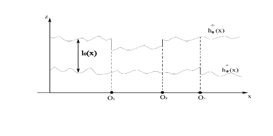
Fig. 2: The case when $l_{0}(x)$ has jumps.

Now we consider in more detail the case when the graph $\Gamma$ does not have any branching but it has many edges $I_{1},...,I_{k},...$ that form a straight line. Let $O_{1},...,O_{k},...$ etc. be the corresponding vertices. Let the corresponding cross-section width be $l_{1}(x),...,l_{k}(x),...$ etc.. (See Fig.2.) In this case the functions $h_{0}^{\pm}(x)$ have jumps. We can introduce a function $l_{0}(x)=l_{k}(x)$ for $A_{k}\leq x\leq B_{k}$. The function $l_{0}(x)$ has jumps at $O_{i}$’s and at the jumps of $l_{0}(x)$ we connect the pieces of the boundary via vertical straight lines. In this way we form the domain $D_{0}$ as we introduced in Section 1. We can find a family of smooth functions $h_{0}^{\pm,\delta}(x)$ such that $h_{0}^{\pm,\delta}(x)$ converge as $\delta\downarrow 0$ uniformly on compact subsets of $\mathbb{R}$ to $h_{0}^{\pm}(x)$. Thus $h_{0}^{+,\delta}(x)-h_{0}^{-,\delta}(x)=l_{0}^{\delta}(x)$ converge as $\delta\downarrow 0$ uniformly on compact subsets of $\mathbb{R}$ to the function $l_{0}(x)$. Also, we can choose such $h_{0}^{\pm,\delta}(x)$ that the domain $D_{0}^{\delta}=\{(x,z):h_{0}^{+,\delta}\leq z\leq h_{0}^{-,\delta}\}$ satisfies our assumptions. Consider the process $\boldsymbol{X}_{t}^{\varepsilon,\delta}$ in the domain $D_{0}^{\delta}$ defined as in (2). Let $Y_{t}^{\varepsilon,\delta}=\mathbf{\mathfrak{Y}}(\boldsymbol{X}_{t}^{\varepsilon,\delta})$. For fixed $\delta>0$, the graph $\Gamma$ corresponding to $Y_{t}^{\varepsilon,\delta}$ has only one edge $I_{1}$. Using the results in Section 2 we see that as $\varepsilon\downarrow 0$ the processes $Y_{t}^{\varepsilon,\delta}$ converge weakly to $Y_{t}^{\delta}$. The process $Y_{t}^{\delta}$ on $\Gamma$ has a generator

$$\overline{L}^{\delta}u(x)=\dfrac{1}{2l_{0}^{\delta}(x)}\dfrac{d}{dx}\left(l_{0}^{\delta}(x)\dfrac{du}{dx}\right)+\overline{V}_{1}^{\delta}(x)\dfrac{du}{dx}\ .$$

Here

$$\overline{V}_{1}^{\delta}(x)=\dfrac{1}{l_{0}^{\delta}(x)}\int_{h_{0}^{-,\delta}(x)}^{h_{0}^{+,\delta}(x)}V(x,z)dz$$

and we have $\overline{V}_{1}^{\delta}(x)\rightarrow\overline{V}_{k}(x)=\beta>0$ as $\delta\rightarrow 0$ uniformly on compact subsets of $x\in\mathbb{R}$.

The above operator can be written in the form of a $D_{v^{\delta}}D_{u^{\delta}}$ operator in the sense of [1]. We can explicitly calculate the functions $u^{\delta}$ and $v^{\delta}$ as follows:

$$u^{\delta}(x)=\int_{0}^{x}\dfrac{1}{l_{0}^{\delta}(y)}\exp\left(-2\int_{0}^{y}\overline{V}_{1}^{\delta}(t)dt\right)dy\ ,$$

$$v^{\delta}(x)=2\int_{0}^{x}l_{0}^{\delta}(y)\exp\left(2\int_{0}^{y}\overline{V}_{1}^{\delta}(t)dt\right)dy\ .$$

Consider a Markov process $Y_{t}^{D_{0}}$ on the graph $\Gamma$. The process $Y_{t}^{D_{0}}$ is governed by the generalized second order differential operator $\overline{L}=D_{v}D_{u}$ (in the sense of [1]) where

$$u(x)=\int_{0}^{x}\dfrac{1}{l_{0}(y)}\exp\left(-2\int_{0}^{y}\overline{V}_{k}(t)dt\right)dy\ ,$$

$$v(x)=2\int_{0}^{x}l_{0}(y)\exp\left(2\int_{0}^{y}\overline{V}_{k}(t)dt\right)dy\ .$$

The domain of definition of the operator $\overline{L}$ consists of those functions $f(x)$ that are continuous and bounded, are twice continuously differentiable and at those points $O_{i}$ where $l_{0}(x)$ have jumps it satisfies a gluing condition $\dfrac{1}{l_{0,-}(O_{i})}f^{\prime}_{-}(O_{i})=\dfrac{1}{l_{0,+}(O_{i})}f^{\prime}_{+}(O_{i})$. Here $l_{0,\pm}(O_{i})$ are the corresponding values of the one sided-limits of $l_{0}(x)$ to the left and to the right of $O_{i}$, and $f^{\prime}_{\pm}(O_{i})$ the corresponding left and right derivatives. The function $\overline{L}f(x)$ is continuous on $\Gamma$.

It follows from the classical result of [6] that we have the following.

Theorem 3. As $\delta\downarrow 0$ the processes $Y_{t}^{\delta}$ converge weakly to the process $Y_{t}^{D_{0}}$ on $\mathbf{C}_{[0,T]}(\Gamma)$.

Let $\tau^{\delta}((-\infty,a])$ be the first time when the process $Y_{t}^{\delta}$ exits from $(-\infty,a]$. Let $\tau^{D_{0}}((-\infty,a])$ be the first time when the process $Y_{t}^{D_{0}}$ exits from $(-\infty,a]$. Weak convergence of processes $Y_{t}^{\delta}$ as $\delta\downarrow 0$ to $Y_{t}^{D_{0}}$ and finiteness of $\mathbf{E}_{0}^{W}\tau^{\delta}((-\infty,a])$ and $\mathbf{E}_{0}^{W}\tau^{D_{0}}((-\infty,a])$ for fixed $\delta>0$ and $a>0$ imply that we have $\lim\limits_{\delta\downarrow 0}\mathbf{E}_{0}^{W}\tau^{\delta}((-\infty,a])=\mathbf{E}_{0}^{W}\tau^{D_{0}}((-\infty,a])$.

We recall the first differential equation we used in the proof of Theorem 2. We plug in $l_{1}(x)=l_{0}^{\delta}(x)$ in that equation and we see that the corresponding solution is just the solution we get there with $l_{1}(x)$ replaced by $l_{0}^{\delta}(x)$. However $\mathbf{E}_{0}^{W}\tau^{\delta}((-\infty,a])$ is the solution of the same problem we used in the proof of Theorem 2 with $l_{1}(x)$ replaced by $l_{0}^{\delta}(x)$ and $\beta$ replaced by $\overline{V}_{1}^{\delta}(x)$. Since $\overline{V}_{1}^{\delta}(x)\rightarrow\beta$ as $\delta\downarrow 0$ we see that we have

$$\begin{array}[]{l}\mathbf{E}_{0}^{W}\tau^{D_{0}}((-\infty,a])=\lim\limits_{\delta\downarrow 0}\mathbf{E}_{0}^{W}\tau^{\delta}((-\infty,a])\\ \displaystyle{=\lim\limits_{\delta\downarrow 0}\left(2\int_{0}^{a}\dfrac{dy}{l_{0}^{\delta}(y)}\int_{0}^{y}l_{0}^{\delta}(t)\exp\left(-2\beta(y-t)\right)dt+2\int_{-\infty}^{0}l_{0}^{\delta}(t)\exp\left(2\beta t\right)dt\int_{0}^{a}\dfrac{1}{l_{0}^{\delta}(y)}\exp\left(-2\beta y\right)dy\right)}\\ \displaystyle{=2\int_{0}^{a}\dfrac{dy}{l_{0}(y)}\int_{0}^{y}l_{0}(t)\exp\left(-2\beta(y-t)\right)dt+2\int_{-\infty}^{0}l_{0}(t)\exp\left(2\beta t\right)dt\int_{0}^{a}\dfrac{1}{l_{0}(y)}\exp\left(-2\beta y\right)dy}\ .\end{array}$$

Following our stationarity and mixing assumptions, after deleting the ”wings”, the remaining channel still satisfies the stationarity and mixing assumptions. Therefore by the same calculation as in the proof of Theorem 2, and using the above formula, we see that we have the following.

Theorem 4. For the process $Y_{t}^{D_{0}}$ defined as above we have

$$\lim\limits_{a\rightarrow\infty}\dfrac{\mathbf{E}_{0}^{W}\tau^{D_{0}}((-\infty,a])}{a}=2\int_{0}^{\infty}K(t)\exp(-2\beta t)dt\ ,$$

where $K(t)=\dfrac{l_{0}(s)}{l_{0}(s+t)}$ and we allow jumps of the function $l_{0}(x)$.

On the other hand, using the same argument of [5] one can show that the process $Y_{t}^{D_{0}}$ can be viewed as the limiting slow motion as $\varepsilon\downarrow 0$ of the part of the process $\boldsymbol{X}_{t}^{\varepsilon}$ within the domain $D_{0}$. To be precise, consider the domain $D$ introduced in Section 1 and the corresponding process $\boldsymbol{X}_{t}^{\varepsilon}$ in $D$. Let $\varphi_{t}=\displaystyle{\int_{0}^{t}\mathbf{1}(\boldsymbol{X}_{s}^{\varepsilon}\in D_{0})ds}$ be an additive functional. (It is called the proper time of the domain $D_{0}$, see [8].) We introduce the time $\beta_{t}$ inverse to $\varphi_{t}$ and continuous on the right. Let $Y_{t}^{\varepsilon,D_{0}}=\mathbf{\mathfrak{Y}}(\boldsymbol{X}_{\beta_{t}}^{\varepsilon})$. Then we can use the same arguments of [5] to prove the weak convergence as $\varepsilon\downarrow 0$ of the processes $Y_{t}^{\varepsilon,D_{0}}$ to the process $Y_{t}^{D_{0}}$.

Consider the process $\boldsymbol{X}_{t}^{\varepsilon}$ moving in the domain $D$ as in Section 1. Let $l_{0}(x)$ be the cross-section width corresponding to the domain $D_{0}$. As before we see that it could have jumps. Let $Y_{t}$ be the limiting slow motion as $\varepsilon\downarrow 0$ of $\boldsymbol{X}_{t}^{\varepsilon}$, defined as in Section 2. Let $\tau((-\infty,a])$ be the first time the process $Y_{t}$ exits from $(-\infty,a]$. Since $Y_{t}$ is the limiting slow motion of $\boldsymbol{X}_{t}^{\varepsilon}$ and $Y_{t}^{D_{0}}$ is the limiting slow motion of the part of $\boldsymbol{X}_{t}^{\varepsilon}$ inside $D_{0}$, we see from the above discussions that we have

$$\tau^{D_{0}}((-\infty,a])=\int_{0}^{\tau((-\infty,a])}\mathbf{1}(\mathbf{\mathfrak{Y}}^{-1}(Y_{t})\subset D_{0})dt\ .$$

By Theorem 4 and the above relation we see that we have the following.

Corollary 1.

$$\lim\limits_{a\rightarrow\infty}\dfrac{\mathbf{E}_{0}^{W}\displaystyle{\int_{0}^{\tau((-\infty,a])}\mathbf{1}(\mathbf{\mathfrak{Y}}^{-1}(Y_{t})\subset D_{0})dt}}{a}=2\int_{0}^{\infty}K(t)\exp(-2\beta t)dt$$

where $K(t)=\mathbf{E}\dfrac{l_{0}(s)}{l_{0}(s+t)}$.

This fact will be used in the next subsection.

4.3 The general case

In the general case when there is branching the domain $D$ consists of a domain $D_{0}$ that has a cross-section width $l_{0}(x)$ which allows occasional jumps. The ”wings” $D_{j}$ ($j\geq 1$) are then attached at the jumps of the domain $D_{0}$.

In this case our graph $\Gamma$ consists of two types of edges. The first type of edges correspond to the domain $D_{0}$ as we discussed in the previous section. The second type of edges correspond to the ”wings” attached to $D_{0}$.

In order to calculate the effective speed of transportation we shall first calculate the expected time that the process spends at one fixed ”wing”. As a first step we do not consider the random shape but perform the calculation for a fixed shape. Also, we shall first consider the simplest case that $\Gamma$ has only three edges: $I_{1}=(-\infty,0]$, $I_{2}=[0,\infty)$ and $I_{3}$ is an edge with one endpoint $O_{1}=0$ and another endpoint $O_{2}=(r,3)$. In this case $l_{1}(x),l_{2}(x)$ and $l_{3}(x)$ are smooth functions.

We construct the process $Y_{t}$ as in Section 2 corresponding to the above graph $\Gamma$. Consider the interval $(-\infty,a]$ for some $a>0$. Let the process $Y_{t}$ start from the point $O_{1}=0$. Let $\tau_{I_{3}}((-\infty,a])$ be the time that the process $Y_{t}$ spends at the edge $I_{3}$ before its first exit time from $(-\infty,a]$. We have the following.

Lemma 1.

$$\mathbf{E}_{0}^{W}\tau_{I_{3}}((-\infty,a])=2\text{sign}(r)\int_{0}^{r}l_{3}(t)\exp(2\beta t)dt\int_{0}^{a}\dfrac{1}{l_{2}(y)}\exp(-2\beta y)dy\ .$$

Proof. Let for example $r>0$. The function $u(x,k)=\mathbf{E}^{W}_{(x,k)}\tau_{I_{3}}((-\infty,a])$ is the solution of the problem

$$\left\{\begin{array}[]{l}\dfrac{1}{2l_{k}(x)}\dfrac{d}{dx}\left(l_{k}(x)\dfrac{du}{dx}\right)+\beta\dfrac{du}{dx}=0\ ,\text{ for }(x,k)\in I_{k}\text{ and }k=1,2\ ,\\ \dfrac{1}{2l_{3}(x)}\dfrac{d}{dx}\left(l_{3}(x)\dfrac{du}{dx}\right)+\beta\dfrac{du}{dx}=-1\ ,\text{ for }(x,3)\in I_{3}\ ,\\ u(-\infty,1)=u(a,2)=0\ ,\\ \lim\limits_{y=(x,3)\rightarrow O_{2}}l_{3}(x)\dfrac{du}{dx}((x,3))=0\ ,\\ l_{1}(0)\lim\limits_{x\rightarrow O_{1}}\dfrac{du}{dx}(x,1)=l_{2}(0)\lim\limits_{x\rightarrow O_{1}}\dfrac{du}{dx}(x,2)+l_{3}(0)\lim\limits_{x\rightarrow O_{1}}\dfrac{du}{dx}(x,3)\ .\end{array}\right.$$

The function $u(x,k)$ is continuous at point $O_{1}$.

Similarly as in Section 4.1 there are solutions $u_{1}(x)=u(x,1),u_{2}(x)=u(x,2)$ and $u_{3}(x)=u(x,3)$ corresponding to the edges $I_{1}$, $I_{2}$ and $I_{3}$. They are defined as follows. We have

$$\begin{array}[]{l}\displaystyle{u_{1}(x)=C_{1}l_{1}(0)\int_{-b}^{x}\dfrac{1}{l_{1}(t)}\exp(-2\beta t)dt+u_{1}(-b)\text{ for }x\in(-\infty,0]\ ,}\end{array}$$

$$\begin{array}[]{l}\displaystyle{u_{2}(x)=C_{2}l_{2}(0)\int_{a}^{x}\dfrac{1}{l_{2}(y)}\exp(-2\beta y)dy\ \text{ for }x\in[0,+\infty)\ ,}\end{array}$$

$$\begin{array}[]{l}\displaystyle{u_{3}(x)=-2\int_{r}^{x}\dfrac{dy}{l_{3}(y)}\left(\int_{0}^{y}l_{3}(t)\exp\left(2\beta(t-y)\right)dt\right)+C_{3}l_{3}(0)\int_{r}^{x}\dfrac{1}{l_{3}(y)}\exp\left(-2\beta y\right)dy+u_{3}(r)}\\ \ \ \ \ \ \ \ \ \ \ \ \ \ \ \ \ \ \ \ \ \ \ \ \ \ \ \ \ \ \ \ \ \ \ \ \ \ \ \ \ \ \ \ \ \ \ \ \ \ \ \ \ \ \ \ \ \ \ \ \ \ \ \ \ \ \ \ \ \ \ \ \ \ \ \ \ \ \ \ \ \ \ \ \ \ \ \text{ for }x\in[0,r]\ .\end{array}$$

We also know that $\lim\limits_{b\rightarrow\infty}u_{1}(-b)=0$. There are $4$ undetermined constants: $C_{1},C_{2},C_{3}$ and $u_{3}(r)$. We can uniquely determine them by the $4$ relations

$$u_{1}(0)=u_{2}(0)=u_{3}(0)\ ,$$

$$\lim\limits_{x\rightarrow r}l_{3}(x)\dfrac{\partial u_{3}}{\partial x}(x)=0\ ,$$

and

$$-l_{1}(0)\dfrac{\partial u_{1}}{\partial x}(0)+l_{2}(0)\dfrac{\partial u_{2}}{\partial x}(0)+l_{3}(0)\dfrac{\partial u_{3}}{\partial x}(0)=0\ .$$

We shall solve the above system. The relations we need are as follows

$$\begin{array}[]{l}\displaystyle{C_{1}l_{1}(0)\int_{-b}^{0}\dfrac{1}{l_{1}(y)}\exp(-2\beta y)dy+u_{1}(-b)}\\ \displaystyle{=-C_{2}l_{2}(0)\int_{0}^{a}\dfrac{1}{l_{2}(y)}\exp(-2\beta y)dy}\\ \displaystyle{=-2\int_{r}^{0}\dfrac{dy}{l_{3}(y)}\left(\int_{0}^{y}l_{3}(t)\exp(2\beta(t-y))dt\right)+C_{3}l_{3}(0)\int_{r}^{0}\dfrac{1}{l_{3}(y)}\exp(-2\beta y)dy+u_{3}(r)\ ,}\end{array}$$

$$-2\int_{0}^{r}l_{3}(t)\exp(2\beta(t-r))dt+C_{3}l_{3}(0)\exp(-2\beta r)=0\ ,$$

$$-C_{1}l_{1}(0)+C_{2}l_{2}(0)+C_{3}l_{3}(0)=0\ .$$

Thus

$$C_{3}l_{3}(0)=2\int_{0}^{r}l_{3}(t)\exp(2\beta t)dt\ .$$

On the other hand, we have

$$C_{1}l_{1}(0)=C_{2}l_{2}(0)+C_{3}l_{3}(0)\ .$$

So we get

$$(C_{2}l_{2}(0)+C_{3}l_{3}(0))\int_{-b}^{0}\dfrac{1}{l_{1}(y)}\exp(-2\beta y)dy+u_{1}(-b)=-C_{2}l_{2}(0)\int_{0}^{a}\dfrac{1}{l_{2}(y)}\exp(-2\beta y)dy\ .$$

This gives us $\lim\limits_{b\rightarrow\infty}(C_{2}l_{2}(0)+C_{3}l_{3}(0))=0$. Thus

$$u_{2}(0)=2\int_{0}^{r}l_{3}(t)\exp(2\beta t)dt\int_{0}^{a}\dfrac{1}{l_{2}(y)}\exp(-2\beta y)dy\ .$$

In the case when $r<0$ the gluing condition becomes

$$l_{1}(0)\lim\limits_{x\rightarrow O_{1}}\dfrac{du}{dx}(x,1)+l_{3}(0)\lim\limits_{x\rightarrow O_{1}}\dfrac{du}{dx}(x,3)=l_{2}(0)\lim\limits_{x\rightarrow O_{1}}\dfrac{du}{dx}(x,2)\ .$$

Thus $C_{1}l_{1}(0)+C_{3}l_{3}(0)=C_{2}l_{2}(0)$. A similar calculation shows that

$$\mathbf{E}_{0}^{W}\tau_{I_{3}}((-\infty,a])=2\int_{r}^{0}l_{3}(t)\exp(2\beta t)dt\int_{0}^{a}\dfrac{1}{l_{2}(y)}\exp(-2\beta y)dy\ .$$

Thus in general we have

$$\mathbf{E}_{0}^{W}\tau_{I_{3}}((-\infty,a])=2\text{sign}(r)\int_{0}^{r}l_{3}(t)\exp(2\beta t)dt\int_{0}^{a}\dfrac{1}{l_{2}(y)}\exp(-2\beta y)dy\ .$$

$\square$

The above lemma can help us to deal with a more general case. Let $q\neq 0$ and $q\in(-\infty,a]$. We assume that the graph $\Gamma$ still consists of $3$ edges $I_{1}=(-\infty,q]$, $I_{2}=[q,\infty)$ and $I_{3}$. In this case the edge $I_{3}$ has one endpoint $O_{1}$ lying on $I_{1}\cup I_{2}$ but with $x$-coordinate $q$, and another endpoint $O_{2}=(q+r,3)$. Let the process $Y_{t}$ again start from the point $0$. (In this case the point $0$ is lying on either $I_{1}$ or $I_{2}$ but may not be on their intersection.) Let $\tau_{I_{3}}((-\infty,a])$ be the time that the process $Y_{t}$ spends at $I_{3}$ before it exits from $(-\infty,a]$. We have the following.

Corollary 2. If $q>0$ then

$$\mathbf{E}_{0}^{W}\tau_{I_{3}}((-\infty,a])=2\text{sign}(r)\int_{q}^{q+r}l_{3}(t)\exp(2\beta(t-q))dt\int_{q}^{a}\dfrac{1}{l_{2}(y)}\exp(-2\beta(y-q))dy\ .$$

If $q<0$ then

$$\mathbf{E}_{0}^{W}\tau_{I_{3}}((-\infty,a])=2\text{sign}(r)\int_{q}^{q+r}l_{3}(t)\exp(2\beta(t-q))dt\int_{0}^{a}\dfrac{1}{l_{2}(y)}\exp(-2\beta(y-q))dy\ .$$

Proof. The above results can be easily seen from the strong Markov property of the process $Y_{t}$ and Lemma 1. To be more precise, if $q>0$, then by strong Markov property $\mathbf{E}_{0}^{W}\tau_{I_{3}}((-\infty,a])$ is just equal to $\mathbf{E}_{q}^{W}\tau_{I_{3}}((-\infty,a])$, which can be calculated using Lemma 1 and a shift. If $q<0$ we need a little bit more argument. In this case we can consider the process $Y_{t}$ starting from $x=q$ and its first time of exiting from $(-\infty,0]$. Let $\tau_{I_{3}}((-\infty,0])$ be the time that $Y_{t}$ spends at $I_{3}$ before it exits from $(-\infty,0]$. Then $\mathbf{E}_{q}^{W}\tau_{I_{3}}((-\infty,0])$ can be calculated using Lemma 1 and a shift. On the other hand, $\mathbf{E}_{q}^{W}\tau_{I_{3}}((-\infty,a])$ can also be calculated using Lemma 1 and a shift. From the strong Markov property of $Y_{t}$ we see that $\mathbf{E}_{0}^{W}\tau_{I_{3}}((-\infty,a])=\mathbf{E}_{q}^{W}\tau_{I_{3}}((-\infty,a])-\mathbf{E}^{W}_{q}\tau_{I_{3}}((-\infty,0])$, which gives the formula we need. $\square$

Following a similar approximation argument as we did in Section 4.2, we can consider the case when the graph $\Gamma$ consists of many edges $I_{1},I_{2},...$ etc. that are of the first type. They correspond to the domain $D_{0}$. We allow jumps of the function $l_{0}(x)$. Then we attach only one ”wing” $D_{1}$ to $D_{0}$ and the domain $D_{1}$ corresponds to an edge $J$ in the graph $\Gamma$. Let $l_{\text{wing}}(x)$, $r$ etc. be the quantities corresponding to the ”wing” $D_{1}$. Let the edge $J$ have two endpoints: $O^{J}_{1}$ lying on $\cup_{k=1}^{\infty}I_{k}$ and with $x$-coordinate $q$; $O^{J}_{2}$ lying on the other endpoint of $J$ with $x$-coordinate $q+r$. After an approximation and averaging we get a process $Y_{t}^{D_{0}\cup D_{1}}$ on $\Gamma$. Let positive $a>q$. Let $\tau_{J}((-\infty,a])$ be the time that the process $Y_{t}^{D_{0}\cup D_{1}}$ spends in the edge $J$ before it exits from $(-\infty,a]$. Lemma 1 and Corollary 2 and the same approximation argument as in Section 4.2 give us the following corollary.

Corollary 3. If $q>0$ then

$$\mathbf{E}_{0}^{W}\tau_{J}((-\infty,a])=2\text{sign}(r)\int_{q}^{q+r}l_{\text{wing}}(t)\exp(2\beta(t-q))dt\int_{q}^{a}\dfrac{1}{l_{0}(y)}\exp(-2\beta(y-q))dy\ .$$

If $q<0$ then

$$\mathbf{E}_{0}^{W}\tau_{J}((-\infty,a])=2\text{sign}(r)\int_{q}^{q+r}l_{\text{wing}}(t)\exp(2\beta(t-q))dt\int_{0}^{a}\dfrac{1}{l_{0}(y)}\exp(-2\beta(y-q))dy\ .$$

If $q=0$ then

$$\mathbf{E}_{0}^{W}\tau_{J}((-\infty,a])=2\text{sign}(r)\int_{0}^{r}l_{\text{wing}}(t)\exp(2\beta t)dt\int_{0}^{a}\dfrac{1}{l_{0}(y)}\exp(-2\beta y)dy\ .$$

Finally we come to the original problem in Section 1. We consider the case when there are many random ”wings” attached to $D_{0}$. Let the process corresponding to the domain $D$ be $\boldsymbol{X}_{t}^{\varepsilon}$. Let the limiting slow motion be $Y_{t}$. We introduce the corresponding quantities $l_{\text{wing}}(x)$, $r$ etc. Let $l_{0}(x)=h_{0}^{+}(x)-h_{0}^{-}(x)$ be the cross section width that corresponds to the domain $D_{0}$. We notice that it has occasional jumps. Let there be $n$ wings in the interval $x\in[0,1]$. We assume that we have the following.

Assumption 7. The random variable $n\geq 1$ is a bounded random variable: $n\leq n_{0}<\infty$.

For $a>0$ we define the random variable

$$M(q,r,a)=\left\{\begin{array}[]{l}\displaystyle{2\text{sign}(r)\int_{q}^{q+r}l_{\text{wing}}(t)\exp(2\beta(t-q))dt\int_{q}^{a}\dfrac{1}{l_{0}(y)}\exp(-2\beta(y-q))dy\ \text{ when }q>0\ ;}\\ \displaystyle{2\text{sign}(r)\int_{q}^{q+r}l_{\text{wing}}(t)\exp(2\beta(t-q))dt\int_{0}^{a}\dfrac{1}{l_{0}(y)}\exp(-2\beta(y-q))dy\ \text{ when }q<0\ ;}\\ \displaystyle{2\text{sign}(r)\int_{0}^{r}l_{\text{wing}}(t)\exp(2\beta t)dt\int_{0}^{a}\dfrac{1}{l_{0}(y)}\exp(-2\beta y)dy\text{ when }q=0}\ .\end{array}\right.$$

We assume that, for some constant $0<A_{1}<\infty$, we have the following.

Assumption 8. $0\leq l_{\text{wing}}(x)\leq A_{1}$ and $|r|\leq A_{1}$.

Thus we see that for some constant $A>0$ we have

$$\left|\int_{0}^{r}l_{\text{wing}}(t)\exp(2\beta t)dt\right|\leq A<\infty\ .$$

We also see that

$$|M(q,r,a)|\leq 2A\int_{0}^{\infty}\dfrac{1}{l_{0}}\exp(-2\beta y)dy\leq M<\infty$$

for some constant $M>0$.

All these random quantities are distributed according to our stationarity and mixing assumptions. Let $\tau((-\infty,a])$ be the first time the process $Y_{t}$ exits from $(-\infty,a]$.

By our assumption on stationarity and mixing, using Corollary 2, we see that we have the following.

Lemma 2. We have

$$\lim\limits_{a\rightarrow\infty}\dfrac{\mathbf{E}_{0}^{W}\displaystyle{\int_{0}^{\tau(-\infty,a]}\mathbf{1}(\mathbf{\mathfrak{Y}}^{-1}(Y_{t})\not\subset D_{0})dt}}{a}=2\mathbf{E}n\mathbf{E}\text{sign}(r)\int_{0}^{r}l_{\text{wing}}(t)\exp(2\beta t)dt\int_{0}^{\infty}\dfrac{1}{l_{0}(y)}\exp(-2\beta y)dy$$

in probability.

Proof. Let the ”wings” located to the left of the point $0$ have $x$-coordinate $0>q_{-1}>q_{-2}>...$. Let the ”wings” located to the right of the point $0$ (including possibly the point $0$) and not exceeding $x=a$ have $x$-coordinate $0\leq q_{1}<...<q_{n(a)}\leq a$. We see that we have

$$\mathbf{E}_{0}^{W}\int_{0}^{\tau(-\infty,a]}\mathbf{1}(\mathbf{\mathfrak{Y}}^{-1}(Y_{t})\not\subset D_{0})dt=\sum\limits_{k=1}^{\infty}M(q_{-k},r_{-k},a)+\sum\limits_{k=1}^{n(a)}M(q_{k},r_{k},a)\ .$$

For $q<0$ we have

$$M(q,r,a)\leq\exp(2\beta q)M(0,r,a)\leq M\exp(2\beta q)\ .$$

Thus

$$\sum\limits_{k=1}^{\infty}M(q_{-k},r_{-k},a)\leq M\sum\limits_{k=1}^{\infty}\exp(2\beta q_{-k})\ .$$

Taking into account Assumption 7 we see that we have

$$\sum\limits_{k=1}^{\infty}\exp(2\beta q_{-k})\leq n_{0}\sum\limits_{k=0}^{\infty}\exp(-2\beta k)<\infty\ .$$

Therefore

$$\lim\limits_{a\rightarrow\infty}\dfrac{\displaystyle{\mathbf{E}_{0}^{W}\int_{0}^{\tau(-\infty,a]}\mathbf{1}(\mathbf{\mathfrak{Y}}^{-1}(Y_{t})\not\subset D_{0})dt}}{a}=\lim\limits_{a\rightarrow\infty}\dfrac{\sum\limits_{k=1}^{n(a)}M(q_{k},r_{k},a)}{a}=\lim\limits_{a\rightarrow\infty}\dfrac{\sum\limits_{k=1}^{n(a)}M(q_{k},r_{k},a)}{n(a)}\dfrac{n(a)}{a}\ .$$

On the other hand, we have

$$\begin{array}[]{l}\displaystyle{\sum\limits_{k=1}^{n(a)}M(q_{k},r_{k},a)}\\ \displaystyle{=\sum\limits_{k=1}^{n(a)}2\text{sign}(r_{k})\int_{q_{k}}^{q_{k}+r_{k}}l_{\text{wing}}(t)\exp(2\beta(t-q_{k}))dt\int_{q_{k}}^{a}\dfrac{1}{l_{0}(y)}\exp(-2\beta(y-q_{k}))dy}\\ \displaystyle{=2\sum\limits_{k=1}^{n(a)}W(q_{k},r_{k})C(q_{k},a)\ .}\end{array}$$

Here

$$W(q_{k},r_{k})=\text{sign}(r_{k})\int_{q_{k}}^{q_{k}+r_{k}}l_{\text{wing}}(t)\exp(2\beta(t-q_{k}))dt$$

and

$$C(q_{k},a)=\int_{q_{k}}^{a}\dfrac{1}{l_{0}(y)}\exp(-2\beta(y-q_{k}))dy\ .$$

Thus we can write

$$\sum\limits_{k=1}^{n(a)}M(q_{k},r_{k},a)=2\sum\limits_{k=1}^{n(a)}W(q_{k},r_{k})C(q_{k},a+q_{k})-2\sum\limits_{k=1}^{n(a)}W(q_{k},r_{k})(C(q_{k},a+q_{k})-C(q_{k},a))\ .$$

By the remark after Assumption 8 we see that

$$\begin{array}[]{l}\displaystyle{2\sum\limits_{k=1}^{n(a)}W(q_{k},r_{k})(C(q_{k},a+q_{k})-C(q_{k},a))}\\ \displaystyle{\leq 2A\sum\limits_{k=1}^{n(a)}(C(q_{k},a+q_{k})-C(q_{k},a))}\\ \displaystyle{\leq\dfrac{2A}{l_{0}}\sum\limits_{k=1}^{n(a)}\int_{a}^{a+q_{k}}\exp(-2\beta(y-q_{k}))dy}\\ \displaystyle{=\dfrac{A}{\beta l_{0}}\sum\limits_{k=1}^{n(a)}[\exp(-2\beta(a-q_{k}))-\exp(-2\beta a)]}\\ \displaystyle{=\dfrac{A}{\beta l_{0}}\sum\limits_{k=1}^{n(a)}\exp(-2\beta(a-q_{k}))-\dfrac{A}{\beta l_{0}}n(a)\exp(-2\beta a)\ .}\end{array}$$

Thus by our Assumption 7 again we see that

$$\lim\limits_{a\rightarrow\infty}\dfrac{2\sum\limits_{k=1}^{n(a)}W(q_{k},r_{k})(C(q_{k},a+q_{k})-C(q_{k},a))}{n(a)}=0\ .$$

Therefore using the weak Law of Large Numbers for triangular arrays and taking into account our assumptions on mixing and stationarity we see that

$$\begin{array}[]{l}\displaystyle{\lim\limits_{a\rightarrow\infty}\dfrac{\sum\limits_{k=1}^{n(a)}M(q_{k},r_{k},a)}{n(a)}}\\ \displaystyle{=2\lim\limits_{a\rightarrow\infty}\dfrac{\sum\limits_{k=1}^{n(a)}W(q_{k},r_{k})C(q_{k},a+q_{k})}{n(a)}}\\ \displaystyle{=2\mathbf{E}\text{sign}(r)\int_{0}^{r}l_{\text{wing}}(t)\exp(2\beta t)dt\int_{0}^{\infty}\dfrac{1}{l_{0}(y)}\exp(-2\beta y)dy}\end{array}$$

in probability.

To be more precise, we write

$$\begin{array}[]{l}\displaystyle{\dfrac{1}{n(a)}\sum\limits_{k=1}^{n(a)}M(q_{k},r_{k},a)}\\ \displaystyle{=\dfrac{1}{n(a)}\sum\limits_{k=1}^{n(a)}(M(q_{k},r_{k},a)-\mathbf{E}M(q_{k},r_{k},a))+\mathbf{E}M(q_{k},r_{k},a)\ .}\end{array}$$

Thus we have

$$\begin{array}[]{l}\displaystyle{\lim\limits_{a\rightarrow\infty}\left(\dfrac{1}{n(a)}\sum\limits_{k=1}^{n(a)}M(q_{k},r_{k},a)\right)}\\ \displaystyle{=\lim\limits_{a\rightarrow\infty}\left(\dfrac{1}{n(a)}\sum\limits_{k=1}^{n(a)}(M(q_{k},r_{k},a)-\mathbf{E}M(q_{k},r_{k},a))\right)+\mathbf{E}M(q_{k},r_{k},\infty)\ .}\end{array}$$

Let $\Phi_{k}(a)=M(q_{k},r_{k},a)-\mathbf{E}M(q_{k},r_{k},a)$. We see that it suffices to prove

$$\lim\limits_{a\rightarrow\infty}\dfrac{1}{n(a)}\sum\limits_{k=1}^{n(a)}\Phi_{k}(a)=0$$

in probability.

Pick any $\delta>0$. By Chebyshev inequality we have the estimate

$$\begin{array}[]{l}\displaystyle{\mathbf{P}\left(\left|\dfrac{1}{n(a)}\sum\limits_{k=1}^{n(a)}\Phi_{k}(a)\right|>\delta\right)}\\ \displaystyle{\leq\dfrac{1}{\delta^{2}n^{2}(a)}\mathbf{E}\left(\sum\limits_{k=1}^{n(a)}\Phi_{k}(a)\right)^{2}}\\ \displaystyle{=\dfrac{1}{\delta^{2}n^{2}(a)}\left(\sum\limits_{k=1}^{n(a)}\mathbf{E}\Phi_{k}^{2}(a)+\sum\limits_{k,l=1,k\neq l}^{n(a)}\mathbf{E}\Phi_{k}(a)\Phi_{l}(a)\right)}\\ \displaystyle{\leq\dfrac{1}{\delta^{2}n^{2}(a)}\left(C_{1}n(a)+C_{2}\sum\limits_{k,l=1,k\neq l}^{n(a)}\exp(-\lambda|q_{k}-q_{l}|)\right)}\ .\end{array}$$

Here by the stationarity assumption we see that $C_{1}=\mathbf{E}\Phi_{k}^{2}(a)$ is a constant. Also, by the exponentially mixing condition we see that $|\mathbf{E}\Phi_{k}(a)\Phi_{l}(a)|=|\mathbf{E}\Phi_{k}(a)\Phi_{l}(a)-\mathbf{E}\Phi_{k}(a)\mathbf{E}\Phi_{l}(a)|\leq C_{2}\exp(-\lambda|q_{k}-q_{l}|)$, $\lambda>0$. By our Assumption 7 we see that

$$\sum\limits_{k,l=1,k\neq l}^{n(a)}\exp(-\lambda|q_{k}-q_{l}|)\leq\sum\limits_{k,l=1,k\neq l}^{n(a)}\exp(-\dfrac{\lambda}{n_{0}}|k-l|)<C_{3}n(a)$$

for some $C_{3}>0$.

Thus for any $\delta>0$ we have

$$\lim\limits_{a\rightarrow\infty}\mathbf{P}\left(\left|\dfrac{1}{n(a)}\sum\limits_{k=1}^{n(a)}\Phi_{k}(a)\right|>\delta\right)=0\ .$$

On the other hand we have $\displaystyle{\lim\limits_{a\rightarrow\infty}\dfrac{n(a)}{a}}=\mathbf{E}n$ almost surely. Thus we can conclude with the final result. $\square$

Adding the two equations in Corollary 1 and Lemma 2 we have the following.

Theorem 5. We have

$$\begin{array}[]{l}\lim\limits_{a\rightarrow\infty}\dfrac{\mathbf{E}_{0}^{W}\tau((-\infty,a])}{a}\\ \\ \displaystyle{=2\int_{0}^{\infty}K(t)\exp(-2\beta t)dt+2\mathbf{E}n\mathbf{E}\text{sign}(r)\int_{0}^{r}l_{\text{wing}}(t)\exp(2\beta t)dt\int_{0}^{\infty}\dfrac{1}{l_{0}(y)}\exp(-2\beta y)dy}\end{array}$$

in probability. Here $K(t)=\mathbf{E}\dfrac{l_{0}(s)}{l_{0}(s+t)}$.

Let $\sigma^{\varepsilon}((-\infty,a])$ be the first time that the process $\boldsymbol{X}_{t}^{\varepsilon}$, starting from a point $\boldsymbol{x}_{0}=(x_{0},z_{0})$ inside $D$, hits the level curve $C(a)$. Since $x_{0}$ is finite we see that Theorems 1 and 5 lead to the following theorem.

Theorem 6. We have

$$\begin{array}[]{l}\lim\limits_{a\rightarrow\infty}\lim\limits_{\varepsilon\downarrow 0}\dfrac{\mathbf{E}_{\boldsymbol{x}_{0}}^{W}\sigma^{\varepsilon}((-\infty,a])}{a}\\ \\ \displaystyle{=2\int_{0}^{\infty}K(t)\exp(-2\beta t)dt+2\mathbf{E}n\mathbf{E}\text{sign}(r)\int_{0}^{r}l_{\text{wing}}(t)\exp(2\beta t)dt\int_{0}^{\infty}\dfrac{1}{l_{0}(y)}\exp(-2\beta y)dy}\end{array}$$

in probability. Here $K(t)=\mathbf{E}\dfrac{l_{0}(s)}{l_{0}(s+t)}$.

The above theorem helps us to conclude in our original problem. We can divide the domain $D\cap\{(x,z):x\in(-\infty,a]\}$ into consecutive pieces alternatively of $x$-length $b$ and $\sqrt{b}$ for some $b>0$. The total time spent by the process $\boldsymbol{X}_{t}^{\varepsilon}$ before it exits from $x=a$ is the sum of those times spent in domains of $x$-length $b$ and those times spent in domains of $x$-length $\sqrt{b}$. As we are taking $a\rightarrow\infty$ we can also let $b\rightarrow\infty$ and the average time spent in domains of $x$-length $\sqrt{b}$ will not contribute. On the other hand, since the process $\boldsymbol{X}_{t}^{\varepsilon}$ has a deterministic positive drift in the $x$-direction, we see that as $b\rightarrow\infty$ the motion inside different domains of $x$-length $b$ will be asymptotically independent. (The motion against the flow is a large deviation effect.) Thus $\sigma^{\varepsilon}((-\infty,a])$ will be asymptotically distributed as the sum of some independent random times. This leads to the relation $\lim\limits_{a\rightarrow\infty}\lim\limits_{\varepsilon\downarrow 0}\dfrac{\mathbf{E}_{\boldsymbol{x}_{0}}^{W}\sigma^{\varepsilon}((-\infty,a])}{a}=\lim\limits_{a\rightarrow\infty}\lim\limits_{\varepsilon\downarrow 0}\dfrac{\sigma^{\varepsilon}((-\infty,a])}{a}$. Thus from Theorem 6 we see that we have the following theorem.

Theorem 7. We have

$$\begin{array}[]{l}\lim\limits_{a\rightarrow\infty}\lim\limits_{\varepsilon\downarrow 0}\dfrac{\sigma^{\varepsilon}((-\infty,a])}{a}\\ \\ \displaystyle{=2\int_{0}^{\infty}K(t)\exp(-2\beta t)dt+2\mathbf{E}n\mathbf{E}\text{sign}(r)\int_{0}^{r}l_{\text{wing}}(t)\exp(2\beta t)dt\int_{0}^{\infty}\dfrac{1}{l_{0}(y)}\exp(-2\beta y)dy}\end{array}$$

in probability. Here $K(t)=\mathbf{E}\dfrac{l_{0}(s)}{l_{0}(s+t)}$.

5 Remarks and generalizations

1. The results of previous sections can be extended to the case of a multidimensional channel $G=\{(x,z):x\in\mathbb{R}^{1},z\in G_{x}\}$ where $G_{x}\subset\mathbb{R}^{n-1}$, $x\in\mathbb{R}^{1}$ are $(n-1)$-dimensional domains assumed to be bounded and consisting of a finite number of connected components; each $G_{x}$ contains the origin. The boundary $\partial G$ of $G\subset\mathbb{R}^{n}$ is assumed to be smooth, except, maybe, a number of $(n-2)$-dimensional manifolds (like the discontinuity points in the $2$-dimensional case). Let $\Gamma$ be the graph homeomorphic (in the natural topology) to the set of connected components of the sets $\{z\in\mathbb{R}^{n-1}:(x,z)\in G\}$ for various $x\in\mathbb{R}^{1}$. Let the functions $l_{i}(x)$ be defined as $(n-1)$-dimensional volumes of corresponding connected components.

Consider the process $\boldsymbol{X}_{t}^{\varepsilon}$ governed by the operator $b\dfrac{\partial}{\partial x}+\dfrac{1}{2}\Delta_{x,z}$ inside the domain $G^{\varepsilon}=\{(x,z):x\in\mathbb{R}^{1},z\in\mathbb{R}^{n-1},(x,z/\varepsilon)\in G\}$. Let $\sigma_{a}^{\varepsilon}=\min\{t:\boldsymbol{X}_{t}^{\varepsilon}\in\{(x,z)\in G\cup\partial G,x=a\}\}$. Then, under mild additional conditions the limit

$$\lim\limits_{a\rightarrow\infty}\lim\limits_{\varepsilon\downarrow 0}\dfrac{\sigma^{\varepsilon}_{a}}{a}$$

exists in probability $\mathbf{P}\times\mathbf{P}_{(x,z)}^{W}$, $(x,z)\in G^{\varepsilon}$ and is given by Theorem 7.

2. Let $\nu_{t}$ be a continuous time Markov chain with $2$ states $1$ and $2$. Let functions $h_{i}^{\pm}(x)$, $x\in\mathbb{R}^{1}$, $i=1,2$, be piecewise smooth, and $h_{i}^{-}(x)<0<h_{i}^{+}(x)$, $x\in\mathbb{R}^{1}$. Put $D_{i}^{\varepsilon}=\{(x,z):x\in\mathbb{R}^{1},-h_{i}^{-}(x)\leq z/\varepsilon\leq h_{i}^{+}(x)\}$ and $D^{\varepsilon}(t)=D_{\nu(t)}^{\varepsilon}$. Define the process $(X_{t}^{\varepsilon},Z_{t}^{\varepsilon})$ in $D^{\varepsilon}(t)$ as the process governed by the operator $b\dfrac{\partial}{\partial x}+\dfrac{1}{2}\Delta_{x,z}$ inside $D^{\varepsilon}(t)$ with the normal reflection on the boundary at the times when $\nu_{t}$ is continuous (then $\nu_{t}$ is constant). Let $Z_{t}^{\varepsilon}$ jump to $0$ at times when $\nu_{t}$ has jumps. (Actually, we need this condition to define the process $(X_{t}^{\varepsilon},Z_{t}^{\varepsilon})$ in a unique way; it is not important since we are interested in the limit as $\varepsilon\downarrow 0$.) Then one can prove that the slow component $X_{t}^{\varepsilon}$ of the process converges as $\varepsilon\downarrow 0$ to the process described by the equation $\dot{X}_{t}=\dot{W}_{t}+\dfrac{1}{2}\widetilde{b}(t,X_{t})$ where $\widetilde{b}(t,x)=b+\dfrac{d}{dx}(\ln l_{\nu_{t}}(x))$, $l_{\nu_{t}}(x)=h_{\nu_{t}}^{+}(x)-h_{\nu_{t}}^{-}(x)$. It is known that for certain drift terms $\widetilde{b}(t,x)$, the process $X_{t}$ demonstrates the so called ratchet effect: If $\nu_{t}$ is identically equal to $1$ or $2$, the process tends to $+\infty$ as $t\rightarrow\infty$, but if $\nu_{t}$ is the Markov chain (independent of $W_{t}$) the process $X_{t}$ tends to $-\infty$.

One can conclude from our considerations, that the ratchet effect can be caused by random and independent of the basic Brownian motion changes of the geometry of the domain.

3. We assumed that the ”wings” have a simple structure – each of them corresponds to just one edge of the graph (Fig.1). One can consider the case of more complicated wings, like, for instance, at the vertex $O_{1}$ in Fig.3. One can also include in the consideration the case when the ”obstacles” in the channel are such that the corresponding graph has loops like that in Fig.3.

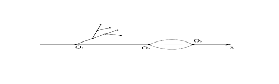
Fig. 3: A more general graph.

If the channel $D^{\varepsilon}$ is not ”uniformly narrow” but has points on axis $x$ such that in the $\delta$-neighborhoods, $\delta=\delta(\varepsilon)<\!<1$ of those points the channel has the ”diameter” of order $\mu(\varepsilon)>\!>\varepsilon$, the limiting process on the graph can have delays or even traps. This will lead to different behavior of $\dfrac{\sigma^{\varepsilon}_{a}}{a}$.

References

- [1] Feller, W., Generalized second-order differential operators and their lateral conditions, Illinois Journal of Mathematics, 1, (1957), pp. 459–504.
- [2] Freidlin, M., Markov Processes and Differential Equations, Asymptotic Problems, Birkhäuser, 1996.
- [3] Freidlin, M., Hu, W., On perturbations of generalized Landau-Lifshitz dynamics, Journal of Statistical Physics, 144, 2011, pp. 978–1008.
- [4] Freidlin, M., Weber M., A remark on random perturbations of nonlinear pendulum, Annals of Applied Probability, 9, 1999, No.3, pp. 611–628.
- [5] Freidlin, M., Wentzell, A., On the Neumann problem for PDE’s with a small parameter and corresponding diffusion processes, Probability Theory and Related Fields, 152 (2012), pp. 101–140.
- [6] Freidlin, M., Wentzell, A., Necessary and Sufficient Conditions for Weak Convergence of One-Dimensional Markov Processes. The Dynkin Festschrift: Markov Processes and their Applications , Birkhauser, (1994) pp. 95–109.
- [7] Jülicher, F., Ajdari, A., Prost, J., Modeling molecular motors, Review of Modern Physics, 69, No. 4, October 1997, pp. 1269–1281.
- [8] Molchanov, S., On a problem in the theory of diffusion processes, Theory of Probability and Its Applications (English translation), 9, 1964, pp. 472–477.