A simple model of the chaotic eccentricity of Mercury

Mercury’s eccentricity is chaotic and can increase so much that collisions with Venus or the Sun become possible. This chaotic behavior results from an intricate network of secular resonances, but in this paper, we show that a simple integrable model with only one degree of freedom is actually able to reproduce the large variations in Mercury’s eccentricity, with the correct amplitude and timescale. We show that this behavior occurs in the vicinity of the separatrices of the resonance $g_{1}-g_{5}$ between the precession frequencies of Mercury and Jupiter. However, the main contribution does not come from the direct interaction between these two planets. It is due to the excitation of Venus’ orbit at Jupiter’s precession frequency $g_{5}$. We use a multipolar model that is not expanded with respect to Mercury’s eccentricity, but because of the proximity of Mercury and Venus, the Hamiltonian is expanded up to order 20 and more in the ratio of semimajor axis. When the effects of Venus’ inclination are added, the system becomes nonintegrable and a chaotic zone appears in the vicinity of the separatrices. In that case, Mercury’s eccentricity can chaotically switch between two regimes characterized by either low-amplitude circulations or high-amplitude librations.

1 Introduction

After the discovery of the chaotic motion of the planets in the Solar System (Laskar, 1989, 1990), it has been demonstrated that the eccentricity of Mercury can rise to very high values (Laskar, 1994), allowing for collision of the planet with Venus. This was confirmed later on by direct numerical integration in simplified models that neglect general relativity (GR) (Laskar, 2008; Batygin & Laughlin, 2008), and even in the full model that includes the GR contribution (Laskar & Gastineau, 2009). Quite surprisingly, the behavior of the system depends strongly on the GR contribution. Indeed, the probability that the eccentricity increases beyond 0.7 in less than 5 Gyr is about 1% in the full model, while it rises to more than 60% when GR is neglected (Laskar, 2008; Laskar & Gastineau, 2009). This behavior is due to the presence of a secular resonance between the perihelion motions of Mercury ($\varpi_{1}$) and Jupiter ($\varpi_{5}$) (Laskar, 2008; Batygin & Laughlin, 2008). Although the origin of the instability in Mercury’s eccentricity is identified, the precise mechanism of the behavior of Mercury’s orbit has not yet been explained in detail. A first attempt was provided by (Lithwick & Wu, 2011), who analyzed the overlap of resonances in the truncated secular Hamiltonian of degree four in eccentricity and inclination. This model reproduces the small diffusion of Mercury’s eccentricity well, and confirms the important role of the $g_{1}-g_{5}$ and $(g_{1}-g_{5})-(s_{1}-s_{2})$ secular resonances between the precession frequency of the perihelion ($g_{i}$) and the regression rate of the ascending node $(s_{i})$. However, Lithwick & Wu (2011) does not explain the steady increase in Mercury’s eccentricity beyond 0.7 as observed in (Laskar, 2008).

In the present paper, our approach is different, since we do not want to be bound to the limitations given by expansions in eccentricity as in (Lithwick & Wu, 2011) or in the previous work of Laskar (1984, 1989, 1990, 2008). As we are looking for a large excursion of the eccentricity of Mercury, we prefer to derive expressions that are valid for all eccentricities, using the averaged expansions derived in (Laskar & Boué, 2010). We provide two simple analytical, secular models. The first one is coplanar with only one degree of freedom. It is thus integrable. This model shows that Mercury’s eccentricity can reach values as high as 0.8 if the system is in the vicinity of the $g_{1}-g_{5}$ resonance. The second model includes inclination and has two degrees of freedom. This spatial model exhibits the chaotic behavior of Mercury’s eccentricity in the neighborhood of the separatrix with possibilities of switching between a regime of moderate eccentricity to a regime of large oscillation where Mercury’s eccentricity reaches very high values. In both models, Mercury is treated as a massless particle, while the motion of the other planets in the Solar System are given by a single term in their quasiperiodic decompositions taken from (Laskar, 1990). In simplified terms, the chaos in Mercury’s orbit is due to the proximity of the resonance with the precession motion of Venus excited at the frequency of Jupiter’s precession frequency.

The secular models that we use in this paper rely on a multipolar expansion of the perturbing function, up to order $(a_{1}/a_{p})^{20}$ in the relativistic case and $(a_{1}/a_{p})^{50}$ in the Newtonian case, where $(a_{p})_{p=2,8}$ are the semimajor axes of the planets of the Solar System in increasing order. This expansion, subsequently averaged over the mean anomalies of all the planets, allows for arbitrary inclinations and eccentricities as long as no orbit crossing occurs.

In section 2, we derive the equations of motion of the coplanar model. This model is very simple with only one degree of freedom associated to Mercury’s eccentricity and longitude of perihelion. Then, in section 3, we derive the possible trajectories in the phase space using level curves of the Hamiltonian for different orders of expansion. We show that it is necessary to develop the perturbing function up to high orders in $(a_{1}/a_{p})$ in order to reach the asymptotic evolution. We also show that the maximum eccentricity attained with an initial eccentricity of $e_{1}=0.2$ is on the order of 0.8 within 4 Myrs as reported in (Laskar, 2008). The spatial case is treated in section 4. This nonintegrable model illustrates the generation of chaos in the vicinitiy of the hyperbolic fixed point of the planar model. We conclude in the last section.

2 Coplanar model

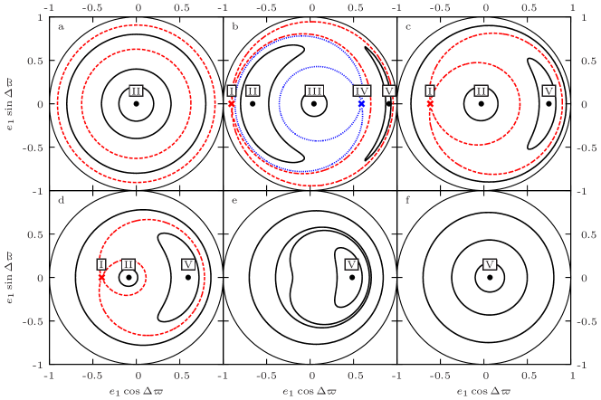
Figure 1: Level curves of the Hamiltonian in the plane $(e_{1}\cos\Delta\varpi,e_{1}\sin\Delta\varpi)$. a) Quadrupole expansion with $g_{1}=5$”/yr. b) Octupole expansion with $g_{1}=5$”/yr. c,d,e,f) expansion up to the order $n=20$ with $g_{1}=2.5,3.6,4.0,5.0$”/yr, respectively.

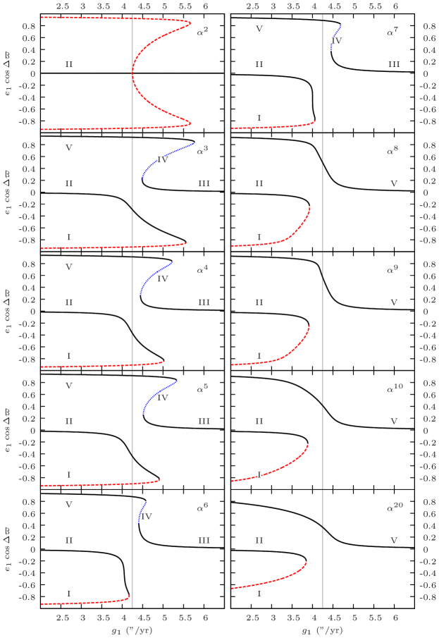
Figure 2: Evolution of the fixed points as a function of the precession frequency of Mercury’s orbit at zero eccentricity and for different expansion orders. Dashed and dotted curves correspond to unstable points, while the solid ones show the positions of the stable points. The equilibrium points are labeled with roman letters as in Fig. 1. The thin vertical line indicates the resonance $g_{1}=g_{5}$.

2.1 Newtonian interaction

Using the traditional notations where planets have increasing indices with respect to their semimajor axis, we note the barycentric position of the Sun $\@vec{u}_{0}$, of Mercury $\@vec{u}_{1}$, of Venus $\@vec{u}_{2}$, etc. The heliocentric positions of the planets are similarly noted $(\@vec{r}_{p})_{p=1,8}$. Since the mass of Mercury is much lower than the masses of the other planets in the Solar System, we model Mercury as a massless particle.

Our goal is to study the behavior of Mercury under a known planetary perturbation. As such, all of the $\@vec{u}_{p}$ and their derivatives, for $p\neq 1$, are considered as given functions of the time $t$. Using the Poincaré heliocentric canonical variables (Laskar & Robutel, 1995), the Hamiltonian describing the evolution of Mercury’s trajectory reads as

$$\hat{H}_{N}=\frac{\tilde{\@vec{r}}_{1}^{2}}{2}-G\frac{m_{0}}{r_{1}}-G\sum_{p=2}^{8}\frac{m_{p}}{\left|\@vec{r}_{1}-\@vec{r}_{p}(t)\right|}+\sum_{p=2}^{8}\frac{m_{p}}{m_{0}}{{\tilde{\@vec{r}}_{1}}\!\cdot\!{\dot{\@vec{u}}_{p}(t)}}\ ,$$ (1)

where $\tilde{\@vec{r}}_{1}=\dot{\@vec{u}}_{1}$ is the conjugate momentum of $\@vec{r}_{1}$, $G$ the gravitational constant, $m_{0}$ the mass of the Sun, and $(m_{p})_{p=2,8}$ the masses of the other planets. The first two terms of this Hamiltonian represent the Keplerian motion and are equal to $-Gm_{0}/(2a_{1})$, where $a_{1}$ is the semimajor axis of Mercury.

Considering that Mercury is the closest planet to the Sun, we now expand $\hat{H}_{N}$ formally as a series in $(r_{1}/r_{p})_{p=2,8}$

$$\hat{H}_{N}=-\frac{Gm_{0}}{2a_{1}}-G\sum_{p=2}^{8}\frac{m_{p}}{r_{p}}\sum_{n=0}^{\infty}\left(\frac{r_{1}}{r_{p}}\right)^{n}P_{n}\left(\frac{{\@vec{r}_{1}}\!\cdot\!{\@vec{r}_{p}}}{r_{1}r_{p}}\right)+\sum_{p=2}^{8}\frac{m_{p}}{m_{0}}{{\tilde{\@vec{r}}_{1}}\!\cdot\!{\dot{\@vec{u}}_{p}}}\ ,$$ (2)

where $P_{n}$ is the Legendre polynomial of order $n$.

A first approximating model could stop the expansion at the second Legendre polynomial $P_{2}$. However, it is well known that the resulting double-averaged secular Hamiltonian does not depend on the perihelia of the outer bodies at this order (Lidov, 1962; Kozai, 1962; Lidov & Ziglin, 1976; Farago & Laskar, 2010), so no secular resonance between the perihelia of Mercury and any other planet can be seen there. We thus push the expansion to higher orders. Furthermore, we see in the following that it is necessary to extend the sum at least up to $n\approx 10$.

The next step consists in averaging the Hamiltonian (2) over the mean anomalies $(M_{p})_{p=1,8}$ of all planets. In the Hamiltonian (2), the terms $-Gm_{0}/r_{p}$ obtained for $n=0$ do not depend on Mercury’s elements; the terms $({\tilde{\@vec{r}}_{1}}\cdot{{\@vec{u}}_{p}})$ vanish when averaged over $M_{1}$; the term $-Gm_{0}/(2a_{1})$ becomes constant after averaging over $M_{1}$, since $a_{1}$ becomes constant. As such, all these terms are dropped in the following expressions. Finally, the averaged expression of the perturbing functions $a_{p}/\left|\@vec{r}_{1}-\@vec{r}_{p}\right|$ are given in (Laskar & Boué, 2010). The resulting Hamiltonian of the coplanar problem is then

$$\hat{H}_{N,{\rm plan}}=-G\sum_{p=2}^{8}\frac{m_{p}}{a_{p}}\sum_{n=2}^{\infty}\left(\frac{a_{1}}{a_{p}}\right)^{n}{\cal F}_{n}^{(0,0)}(e_{1},e_{p},\varpi_{1}-\varpi_{p})\ ,$$ (3)

where

$${\displaystyle{\cal F}_{n}^{(0,0)}(e_{1},e_{p},\varpi)=\epsilon_{n}f_{n,\frac{n}{2}}X_{0}^{n,0}(e_{1})X_{0}^{-(n+1),0}(e_{p})}$$

(4)

In these expressions, $a_{p}$, $e_{p}$, and $\varpi_{p}$ are the semimajor axis, the eccentricity, and the longitude of the pericenter of the planet $p$, respectively. The $X_{k}^{n,m}(e)$ are the Hansen coefficients defined by

$$\left(\frac{r}{a}\right)^{n}{\rm e}^{imv}=\sum_{k=-\infty}^{\infty}X_{k}^{n,m}(e){\rm e}^{ikM}\ ,$$ (5)

where $\epsilon_{n}=0$ if $n$ is odd, and $\epsilon_{n}=1$ if $n$ is even, and

$$f_{n,q}=\frac{(2q)!(2n-2q)!}{2^{2n}(q!)^{2}((n-q)!)^{2}}\ .$$ (6)

To simplify the expansion of the Hamiltonian (2), we take advantage of the eccentricities $(e_{p})_{p=2,8}$ of all the planets beyond Mercury remaining low to only keep the linear terms in these eccentricities. In contrast, the expansion remains exact in the eccentricity $e_{1}$. With this approximation, up to the octupole order, the averaged Hamiltonian (2) reads as

$${\displaystyle\hat{H}_{N,{\rm plan}}\approx-\frac{G}{8}\sum_{p=2}^{8}}$$

(7)

More generally, as long as the Hamiltonian is truncated at the first order in $e_{p}$, its expression can be written as (see Appendix A)

$${\displaystyle\hat{H}_{N,{\rm plan}}=-G\sum_{p=2}^{8}\frac{m_{p}}{a_{p}}\bigg{(}}$$

(8)

where ${\rm P}_{\alpha}\!(\alpha,x)$ and ${\rm Q}_{\alpha}\!(\alpha,x)$ are polynomials of degree $[n/2]$ and $[(n-1)/2]$ in $x$ and of degree $2[n/2]$ and $2[(n+1)/2]-1$ in $\alpha$, with $n$ the degree of expansion of the perturbing functions as in Eq. (3). It can be noted that the coefficient of $x^{0}$ in ${\rm P}_{\alpha}\!(\alpha,x)$ is the Taylor expansion of $C_{1}(\alpha)-1=(1/2)b_{1/2}^{(0)}(\alpha)$ -1, and the coefficient of $x^{1}$ in ${\rm P}_{\alpha}\!(\alpha,x)$ is the Taylor series of $C_{3}(\alpha)/2=(1/8)\alpha b_{3/2}^{(1)}(\alpha)$, etc., where $b_{s}^{(k)}(\alpha)$ are Laplace coefficients (Laskar & Robutel, 1995).

In the Hamiltonian (8), $e_{p}$ and $\varpi_{p}$ are functions of time. Neglecting the slow diffusion of the eccentricities of the inner planets, the evolution of each $z_{p}=e_{p}\exp i\varpi_{p}$ is described well by a quasiperiodic expansion (Laskar, 1990). In this study, we focus on the secular resonance $g_{1}-g_{5}$. In the quasiperiodic decomposition of the variables $(z_{p})_{p=2,8}$, we thus keep only the terms associated to the eigenmode $z_{5}^{\star}=\exp ig_{5}t$ with frequency $g_{5}\approx 4.25$”/yr. The others average out and disappear from the Hamiltonian.

Table 1: Amplitude of the quadrupole $\varepsilon_{p}^{\rm quad}$ (14) and octupole $\varepsilon_{p}^{\rm octu}$ (13) terms, due to each planet $p$, amplitude $A_{p}$, and phase $\varphi_{p}$ of the eigenmode with frequency $g_{5}=4.2488163$”/yr in the quasiperiodic decomposition of $z_{p}=e_{p}\exp i\varpi_{p}$ (taken from Laskar, 1990).

$p$	$\varepsilon_{p}^{\rm quad}\times 10^{6}$	$\varepsilon_{p}^{\rm octu}\times 10^{6}$	$A_{p}\times 10^{6}$	$\varphi_{p}$ (deg.)
2	59 375	1 170	19 636	30.571
3	27 911	383	18 913	30.597
4	837	8	20 300	30.679
5	62 201	383	44 119	30.676
6	3 025	8	33 142	30.676
7	57	0	37 351	210.671
8	17	0	1 771	30.669

The amplitude and the phase of the mode $z_{5}^{\star}$ in the decomposition of each variable $z_{p}$ are provided in Table 1. We notice that, except for Uranus ($p=7$), all the phases are the same and equal to $\approx 30.6\deg$. Since, $\varphi_{7}=30.6+180\deg$, it is equivalent to take $\varphi^{\prime}_{7}=30.6\deg$ and $A^{\prime}_{7}=-A_{7}$. This is the convention that is followed hereafter, but the prime is omitted for clarity. We note $\varpi_{5}^{\star}=g_{5}t+\varphi_{5}^{\star}$, where $\varphi_{5}^{\star}=30.6\deg$. We also use the fact that $\Lambda_{1}=\sqrt{Gm_{0}a_{1}}$ is constant in the secular problem to rescale the Hamiltonian by this quantity as it simplifies the following expressions. We note $\check{H}_{N,{\rm plan}}=\hat{H}_{N,{\rm plan}}/\Lambda_{1}\ .$ Given that $Gm_{p}/(\Lambda_{1}a_{p})=n_{1}a_{1}m_{p}/(a_{p}m_{0})\ ,$ the resonant Hamiltonian now reads as

$${\displaystyle\check{H}_{N,{\rm plan}}=-n_{1}\sum_{p=2}^{8}}$$

(9)

With this convention, the time should also be rescaled by the same factor $\Lambda_{1}$ to keep the canonical form of the equations of motion, unless the canonical variables are modified as follows. We let

$${\displaystyle\hat{I}=\Lambda_{1}\left(1-\sqrt{1-e_{1}^{2}}\right)\ ,}$$

(10)

be the canonical conjugated variables of the initial Hamiltonian $\hat{H}_{N,{\rm plan}}$ of (Eq.8). It can be easily shown that

$$(\check{I},\check{\theta})=\left(\frac{\hat{I}}{\Lambda_{1}},\hat{\theta}\right)$$ (11)

are canonical conjugated variables of the Hamiltonian $\check{H}_{N,{\rm plan}}$ (Eq.9) without rescaling the time $t$. The equations of motion are thus

$${\displaystyle\frac{d\check{I}}{dt}}$$

(12)

At this point, it is interesting to evaluate the contribution of each planet to the octupole interaction with Mercury. Although the resonance $g_{1}-g_{5}$ involves only the precession frequencies associated to Mercury and Jupiter, the eigenmode $z_{5}^{\star}$ is present in the quasiperiodic decomposition of the motion of all the planets. Furthermore, the amplitudes of this mode are very similar and vary only within a factor 2.5 between 0.019 and 0.044, except for Neptune whose amplitude is only 0.002 (Table 1). From the expression of the Hamiltonian (9), knowing that the lowest degree of $Q(\alpha,x)$ in $\alpha$ is 3, the contribution of the octupole terms can be estimated using the parameters $(\varepsilon^{\rm octu}_{p})_{p=2,8}$ given by

$$\varepsilon_{p}^{\rm octu}=\frac{15}{64}\left(\frac{n_{1}}{g_{5}}\right)\left(\frac{m_{p}}{m_{0}}\right)\left(\frac{a_{1}}{a_{p}}\right)^{4}A_{p}\ .$$ (13)

The values taken by these parameters are gathered in Table 1. The maximal amplitude is due to Venus with $\varepsilon_{2}^{\rm octu}\approx 0.0012$ followed by the Earth-Moon barycenter and Jupiter with $\varepsilon_{3}^{\rm octu}\approx\varepsilon_{5}^{\rm octu}\approx 4\times 10^{-4}$. Thus, the strongest perturbation on Mercury’s orbit comes from the precession of Venus excited by Jupiter. $a_{1}/a_{2}\approx 0.53$ is not very small explains why it is necessary to perform the expansion of the perturbing function up to a high order in the ratio of the semimajor axes. For completeness, Table 1 also provides the quadrupole contribution of each planet given by

$$\varepsilon_{p}^{\rm quad}=\frac{1}{8}\left(\frac{n_{1}}{g_{5}}\right)\left(\frac{m_{p}}{m_{0}}\right)\left(\frac{a_{1}}{a_{p}}\right)^{3}\ .$$ (14)

Since we have shown that several planets play a role in the evolution of Mercury’s eccentricity, in the following we always consider all the perturbers from Venus to Neptune. To simplify the notations, we define two new polynomials ${\rm P}$ and ${\rm Q}$ of the eccentricity $e_{1}$ alone, given by (Eq. 9)

$${\displaystyle{\rm P}(x)}$$

(15)

Then, the resonant Hamiltonian (9) reads as

$$\check{H}_{N,{\rm plan}}=-g_{5}\big{(}{\rm P}(e_{1}^{2})-e_{1}{\rm Q}(e_{1}^{2})\cos(\varpi_{1}-\varpi_{5}^{\star})\big{)}\ .$$ (16)

The numerical values of the coefficients of the polynomials ${\rm P}$ and ${\rm Q}$ are given in Appendix B.

The Hamiltonian $\check{H}_{N,{\rm plan}}$ (16) has one and a half degrees of freedom, but it can be reduced to a one degree of freedom Hamiltonian $\tilde{H}_{N,{\rm plan}}$ after some modifications. For that, we first make the Hamiltonian autonomous by a adding a momentum $\check{T}$ conjugated to time $t$. Then, we perform a canonical transformation where the old variables are

$$(\check{I}=1-\sqrt{1-e_{1}^{2}}\ ,\check{\theta}=-\varpi_{1})\ ;\quad(\check{T}\ ,t)\ ,$$ (17)

and the new ones are $(I,\Delta\varpi)$ and $(\tilde{T},\tilde{t})$, defined by

$${\displaystyle\Delta\varpi=-\check{\theta}-g_{5}t-\varphi_{5}^{\star}\equiv\varpi_{1}-\varpi_{5}^{\star}\ ,}$$

(18)

For this transformation to be canonical, the momentums should verify

$${\displaystyle\check{I}=-I\equiv 1-\sqrt{1-e_{1}^{2}}\ ,}$$

(19)

The new Hamiltonian $\tilde{H}_{N,{\rm plan}}$ expressed in the new variables does not depend on the cyclic coordinate $\tilde{t}$. Thus, its conjugated momentum $\tilde{T}$ is an integral of the motion and can be dropped. Up to a constant, the new Hamiltonian is then

$$\tilde{H}_{N,{\rm plan}}=-g_{5}\sqrt{1-e_{1}^{2}}-g_{5}{\rm P}\left(e_{1}^{2}\right)+g_{5}e_{1}{\rm Q}\left(e_{1}^{2}\right)\cos\Delta\varpi\ .$$ (20)

This one degree of freedom Hamiltonian is integrable. The orbits are given by $\tilde{H}_{N,{\rm plan}}=Cte$. The temporal evolution of the eccentricity $e_{1}$ and of the resonant angle $\Delta\varpi$ are deduced from the canonical equations of motion. This leads to

$${\displaystyle\frac{de_{1}}{dt}}$$

(21)

2.2 General relativistic precession

The secular effect of relativity is described by (e.g., Touma et al., 2009),

$$H_{R}=-g_{r}\frac{1}{\sqrt{1-e_{1}^{2}}}\ ,$$ (22)

where $g_{r}=3(Gm_{0})^{2}/(\Lambda_{1}a_{1}^{2}c^{2})$, and $c$ is the speed of light. In the case of Mercury, we have $g_{r}\approx 0.41$”/yr. The total Hamiltonian $\tilde{H}_{R,{\rm plan}}=\tilde{H}_{N,{\rm plan}}+H_{R}$, including the Newtonian interaction and general relativity, becomes

$${\displaystyle\tilde{H}_{R,{\rm plan}}=}$$

(23)

2.3 Additional control term

Using the Newtonian Hamiltonian (20), or the relativistic one (23), the system is far from the $g_{1}-g_{5}$ resonance, in a configuration where the amplitude of oscillation of the eccentricity is small (see next section). Indeed, taking an order of expansion $n=50$, we get $g_{1}=5.54$”/yr in the Newtonian case and $g_{1}=5.96$”/yr in the relativistic case, whereas the resonance occurs in the vicinity of $g_{1}=g_{5}=4.25$”/yr. This result is slightly different, but representative of the present behavior of Mercury’s eccentricity. Indeed, the present value of $g_{1}$ for the Solar System with GR is $g_{1}=5.59$”/yr (Laskar et al., 2004), the differences with the present model being due to the simplifications that are made here. To recover a model that is dynamically close to the real Solar System, we add a correction to the Hamiltonian which changes the value of $g_{1}$ by an increment $\delta_{g}$. In addition, owing to the slow chaotic diffusion in the inner Solar System, Mercury’s precession frequency $g_{1}$ can change quasi-randomly and come close to the value of $g_{5}$, then leading to high unstability (Laskar, 1990, 2008; Batygin & Laughlin, 2008; Laskar & Gastineau, 2009). To explore the evolution of Mercury’s eccentricity for different values of $g_{1}$ around the resonant frequency $g_{5}$, the above-mentioned correction is added to both $\tilde{H}_{N,{\rm plan}}$ and $\tilde{H}_{R,{\rm plan}}$; i.e.,

$$H_{N,{\rm plan}}=\tilde{H}_{N,{\rm plan}}+\frac{1}{2}\delta_{g}e_{1}^{2}$$ (24)

and

$$H_{R,{\rm plan}}=\tilde{H}_{R,{\rm plan}}+\frac{1}{2}\delta_{g}e_{1}^{2}\ .$$ (25)

In Eqs. (24) and (25), the factor $\delta_{g}$ controls the precession frequency $g_{1}$. For $\delta_{g}=0$, we recover the values obtained with $\tilde{H}_{N,{\rm plan}}$ and $\tilde{H}_{R,{\rm plan}}$, respectively. Otherwise the value of $g_{1}$ is incremented by $\delta_{g}$. Appendix C provides the values of $\delta_{g}$ that put the system in exact resonance for all orders of expansion of the Hamiltonians.

3 Eccentricity behavior

Here, we analyze the possible trajectories and evolutions of Mercury’s eccentricity described by the Hamiltonians $H_{N,{\rm plan}}$ (24) and $H_{R,{\rm plan}}$ (25) obtained in the previous section. Since these Hamiltonians are integrable (they have only one degree of freedom), all the orbits are necessarily regular. Thus, the goal of this section is not to reproduce the chaotic behavior of Mercury’s eccentricity $e_{1}$, but to show that $e_{1}$ can actually reach values as high as observed by Laskar (2008) (see Fig. 3a) when the system is in the vicinity of the resonance $g_{1}=g_{5}$. The chaotic evolution will be analyzed in the spatial case (see Sect. 4), where a new degree of freedom is added.

3.1 Dependency with the order of expansion

The Hamiltonians of the previous section have been computed as series in power of the semimajor axis ratios $(a_{1}/a_{p})_{p=2,8}$ for any order $n$. Here, we study the effect of the truncation of these series. Hereafter, we note with a superscript $(n)$ any Hamiltonian expanded up to the order $n$, e.g., $H_{N,{\rm plan}}^{(n)}$ or $H_{R,{\rm plan}}^{(n)}$. In a first step, we focus only on the relativistic Hamiltonian which is more complete.

Within the quadrupole approximation, the Hamiltonian $H_{R,{\rm plan}}^{(2)}$ reduces to a simple expression

$${\displaystyle H_{R,{\rm plan}}^{(2)}=}$$

(26)

where $\varepsilon^{\rm quad}=\sum_{p}\varepsilon^{\rm quad}_{p}$. This Hamiltonian is independent of $\Delta\varpi$, thus $e_{1}$ remains constant. All the trajectories in the plane ($x=e_{1}\cos\Delta\varpi$, $y=e_{1}\sin\Delta\varpi$) are circles centered on the origin (0,0) with an eventually infinite period when $\Delta\dot{\varpi}=0$. Figure 1a illustrates this result for $g_{1}=5$”/yr. The position of the fixed points is represented by red dashed curves. Within this approximation, as noted before, there is no possible resonance between $\varpi_{1}$ and $\varpi_{5}^{\star}$ and thus, no possible increase in the eccentricity.

The next level of approximation is the octupole. The corresponding Hamiltonian reads as

$${\displaystyle H_{R,{\rm plan}}^{(3)}=}$$

(27)

with $\varepsilon^{octu}=\sum_{p}\varepsilon^{\rm octu}_{p}$. In that case the phase space can be much more complicated with five fixed points and two sets of separatrices (see Fig. 1b obtained with $g_{1}=5$”/yr). The stable fixed points are represented by black dots, and the unstable ones are noted with crosses. The dashed curves correspond to the separatrices. The positions and existence of the fixed points depend on the value of the precession frequency $g_{1}$. This is depicted in the subpanel labeled $\alpha^{3}$ of Fig. 2. The curves represent the position on the $x$ axis of the fixed points of the phase space as a function of $g_{1}$. The labels in roman numerals qualifying each fixed point are identical to those in Fig. 1.

Figure 3: Comparison between the eccentricity evolution observed in (Laskar, 2008) (a), and produced by the simple model of this work (b).

It is interesting to have a look at all of Fig. 2. Indeed, as the order $n$ of the expansion of the Hamiltonian $H_{R,{\rm plan}}^{(n)}$ increases, the degrees of the polynomials ${\rm P}_{\alpha}\!(\alpha,e^{2})$ and ${\rm Q}_{\alpha}\!(\alpha,e^{2})$ increase both for $\alpha$ and $e^{2}$. Then, the topology of the phase space of the Hamiltonian $H_{R,{\rm plan}}^{(n)}$ evolves as shown in Fig. 2. Up to $n=5$, five fix points – three stable points and two unstable points – coexist within $4.5\lesssim g_{1}\lesssim 5.0$”/yr, while the system contains at most three fix points – two stable points and one unstable point – for $n\geq 6$. Moreover, the hyperbolic point (labeled IV) located at $e_{1}\cos\Delta\varpi>0$, i.e. $\Delta\varpi=0$, disappears when $n\geq 8$. The asymptotic topology is reached at $n\approx 10$ from which positions of the fixed points do not evolve significantly up to $n=20$.

The figures 1c, 1d, 1e, and 1f display the allowed trajectories of Mercury’s eccentricity for $n=20$ which is assumed to be representative of the asymptotic behavior. The values of $g_{1}$ are 2.5, 3.6, 4.0, and 5.0”/yr, respectively. At this order $n=20$, orbits are very similar to those of a simple pendulum with a large resonant island allowing for large increases in eccentricity beyond $e_{1}=0.8$. The separatrix disappears at $g_{1}\geq 3.84$”/yr but high eccentricity excursions are still possible, to a smaller extent, since the elliptic fixed point (V) remains significantly offset with respect to the center of the phase space as long as $g_{1}\lesssim 4.5$”/yr. For example, with $g_{1}=4.0$”/yr (Fig. 1e), a trajectory starting within $e_{1}\leq 0.2$ can reach $e_{1}\approx 0.7$.

To conclude, the asymptotic phase space, which must reproduce Mercury’s eccentricity behavior as faithfully as possible, is obtained for $n\approx 20$. Moreover, at this order of expansion, Mercury’s eccentricity is able to increase from $e_{1}\approx 0.2$ up to $e_{1}\approx 0.8$ as observed in the numerical simulations reported by Laskar (2008) (see Fig. 3).

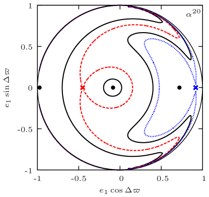
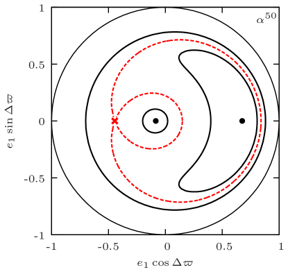
Figure 4: Level curves of the Hamiltonian without relativity in the plane $(e_{1}\cos\Delta\varpi,e_{1}\sin\Delta\varpi)$ for two orders of expansion: $n=20$ (left), $n=50$ (right). In both cases, $g_{1}=3.6$”/yr.

3.2 Temporal evolution

The level curves of the Hamiltonian $H_{R,{\rm plan}}^{(20)}$ provide the trajectories of Mercury’s eccentricity in the phase space. In the previous section, we saw that the eccentricity is able to vary between 0.2 and 0.8 as observed in (Laskar, 2008) (Fig. 3a). We now check whether the timescale of the evolution matches the 4 Myr found by Laskar (2008). For this purpose, we integrate the following equations

$${\displaystyle\frac{dx}{dt}=}$$

(28)

where $x=e_{1}\cos\Delta\varpi$ and $y=e_{1}\sin\Delta\varpi$. They are equivalent to the equations of motion (21), but without singularities at the origin $e_{1}=0$.

An example of temporal evolution given by the numerical integration of Eq. (28) is displayed in Fig. 3b. The initial conditions are $e_{1}=0.2$, $\Delta\varpi=110\deg$, and $g_{1}=3.68$”/yr. The comparison of Fig. 3a with Fig. 3b shows that the simple one degree of freedom model described in this study is able to reproduce the main evolution of Mercury’s eccentricity with the correct amplitude and timescale. Only once the eccentricity reaches a value close to 0.8, Mercury’s orbit becomes highly unstable due to close encounters with Venus, and the evolution observed in (Laskar, 2008) starts to differ significantly from the simple model. It should be noted that the small oscillations present in the integration of the full Solar System (Fig. 3a) do not appear in the simple model since we keep only one single eigen frequency to describe the evolution of the outer planets eccentricities.

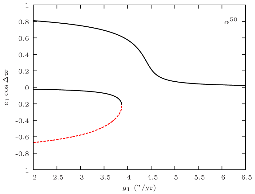
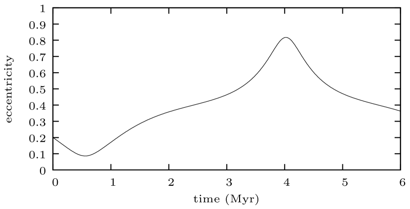
Figure 5: Top: evolution of the fixed points of $H^{(50)}$ without relativity. Bottom: evolution of the eccentricity with time, using the simple model without relativity.

3.3 Without relativity

We now consider the evolution of Mercury’s eccentricity without general relativity, i.e., described by the Hamiltonian $H_{N,{\rm plan}}^{(n)}$ (24). Figure 4 shows the level curves of $H_{N,{\rm plan}}^{(20)}$ and $H_{N,{\rm plan}}^{(50)}$. The two figures are similar to the subpanel $\alpha^{20}$ of Fig. 1 within the region of low eccentricities ($e_{1}\lesssim 0.6$). But for higher eccentricities, two new fixed points appear in the Newtonian case with $n=20$. It is then necessary to extend the expansion up to the order $n\approx 50$ to get the asymptotic topology of the phase space. Once the limit is closely reached, the result matches the relativistic ones well. The only difference is in the value of $\delta_{g}$: for a given frequency $g_{1}$, it should be increased by $g_{r}=0.41$”/yr with respect to the relativistic case (see Table 3).

Figure 5 shows the positions of the fixed points and the temporal evolution of the eccentricity driven by $H_{N,{\rm plan}}^{(50)}$. There is no significant difference with respect to the relativistic case.

4 Spatial model

The evolutions studied in the previous sections are perfectly regular. Indeed, the Hamiltonian contains only one degree of freedom and is thus integrable. The goal was to show that it is possible to explain the large increase in Mercury’s eccentricity observed in numerical simulations (e.g., Laskar, 2008). Our aim is now to introduce an additional degree of freedom to make the system non integrable and to reproduce a chaotic evolution expected in the vicinity of the separatrix of the $g_{1}-g_{5}$ resonance.

To do so, we add inclination in our system, and focus on the term related to $(g_{1}-g_{5})-(s_{1}-s_{2})$. This resonant term is at present in libration, and was identified as one of the main source of chaos in the Solar System (Laskar, 1990). It was indeed also computed analytically in (Laskar, 1984), where it was identified as the major obstacle for the convergence of the secular perturbation series. The Hamiltonian of the inclined problem is (see Appendix D)

$${\displaystyle\check{H}_{R,{\rm inc}}=}$$

(29)

where $i_{p}$ and $\Omega_{p}$ are the inclination and the longitude of the ascending node of the planet $p$, and $I_{p}$ and $\Omega_{2}^{\star}$ are the amplitude and the argument of the term precessing at the frequency $s_{2}$ in the quasiperiodic decomposition of $\sin(i_{p}/2)\exp({\rm i}\Omega_{p})$, respectively. In (29), both $\varpi_{5}^{\star}=g_{5}t+\varphi_{5}^{\star}$ and $\Omega_{2}^{\star}=s_{2}t+\phi_{2}^{\star}$ are functions of time $t$. To reduce the number of degrees of freedom from 2.5 to 2, we apply transformations similar to those of the planar case (Sect. 2). We first add to the Hamiltonian the momentum $\check{T}$ conjugated to the time $t$. The old variables of the subsequent canonical transformation are

$${\displaystyle\check{I}=1-\sqrt{1-e_{1}^{2}}\ ,\quad}$$

(30)

and the new variables are denoted $(I,\Delta\varpi)$, $(J,\Delta\Omega)$, $(\tilde{T},\tilde{t})$. We set

$${\displaystyle\Delta\varpi=-\check{\theta}-g_{5}t-\varphi_{5}^{\star}\equiv\varpi_{1}-\varpi_{5}^{\star}\ ,}$$

(31)

The associated conjugated momenta are given by

$${\displaystyle\check{I}=-I\ ,}$$

(32)

Since the new Hamiltonian $\tilde{H}_{R,{\rm inc}}$ is independent of $t$, its conjugate momentum $\tilde{T}$ is an integral of the motion. From the expressions of $\check{I}$ and $\check{J}$ (30), we thus get, up to a constant,

$${\displaystyle\tilde{H}_{R,{\rm inc}}}$$

(33)

To obtain the final Hamiltonian $H_{R,{\rm inc}}$ in the spatial case, we add the control term and get

$$H_{R,{\rm inc}}=\tilde{H}_{R,{\rm inc}}+\frac{1}{2}\delta_{g}e_{1}^{2}\ .$$ (34)

The Hamiltonian (34) now has two degrees of freedom. The variables are $(e_{1},\Delta\varpi)$ and $(i_{1},\Delta\Omega)$. To perform numerical integrations, we use nonsingular rectangular coordinates

$${\displaystyle k=e_{1}\cos\Delta\varpi\ ,\quad}$$

(35)

With $\chi=\sqrt{1-e_{1}^{2}}$, the equations of motion read as (e.g. Bretagnon, 1974)

$${\displaystyle\frac{dk}{dt}}$$

(36)

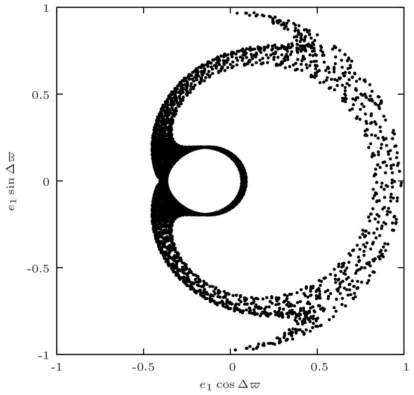
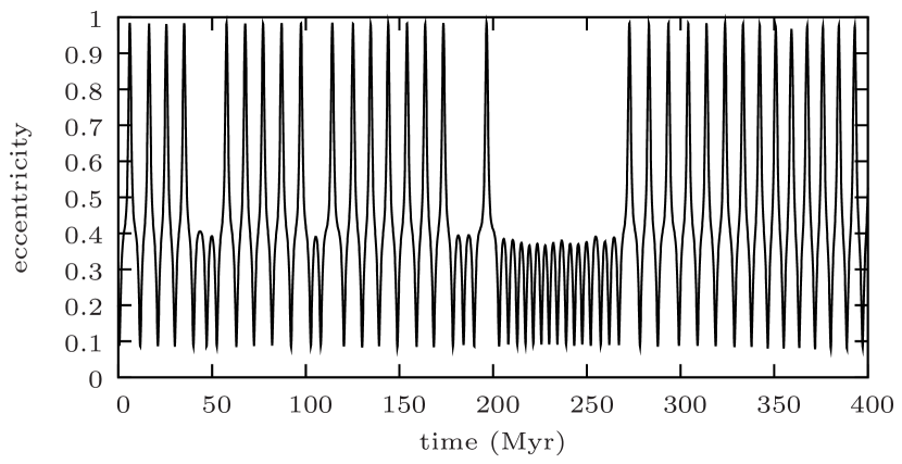
Figure 6: Top: trajectory of Mercury’s eccentricity in the plane $(e_{1}\cos\Delta\varpi,e_{1}\sin\Delta\varpi)$ for the inclined system. Bottom: evolution of Mercury’s eccentricity as a function of time in the same system.

Since Venus is the only planet with a significative amplitude associated to the frequency $s_{2}$, it is also the only planet for which the inclination is taken into account. The initial inclination of Mercury is taken from (Laskar, 1990) where all the terms in its frequency decomposition, except the constant one, have been added. Doing so, Mercury’s initial inclination is measured with respect to the invariant plane.

Figure 6 shows the results of a numerical integration of the inclined system. A large chaotic zone appears in the vicinity of the separatrix, as expected. Mercury’s eccentricity now switches randomly between low-amplitude circulations and high-amplitude excursions, reaching values that are close to 1.

It should ne noted that the Solar System is not presently in this chaotic zone. As described elsewhere (Laskar, 1990, 2008; Batygin & Laughlin, 2008; Laskar & Gastineau, 2009; Lithwick & Wu, 2011), the system is at present in a secular resonance (with resonant argument $(g_{1}-g_{5})-(s_{1}-s_{2})$), in a state of slow chaos, with slow chaotic diffusion. This diffusion will quasi-randomly change the value of $g_{1}$, which can then approach resonance with $g_{5}$. The phase diagram of Fig. 6 describes the behavior of Mercury’s eccentricity once this slow diffusion has brought the system into the vicinity of the $g_{1}-g_{5}$ resonance.

5 Conclusion

In this study, we developed a simple model to account for the increase in Mercury’s eccentricity due to the resonance $g_{1}=g_{5}$. This coplanar model is based on the expansion of the perturbing function with respect to the semimajor axis ratios, and exact in eccentricity. In the resulting Hamiltonian, we kept only one term in the quasiperiodic evolution of the outer planets’ eccentricity. We found that this approximation is sufficient to reproduce an increase in Mercury’s eccentricity up to 0.8. But we also noticed that it is necessary to extend the expansion up to the order $n\approx 20$ and $n\approx 50$ in the relativistic and in the Newtonian cases, respectively. The explicit form of this secular resonant Hamiltonian is provided in Appendix B.

The asymptotic topologies of the phase space are very similar no matter whether the relativity is taken into account or not, so these two cases just depend on the value of the resonant frequency (Table 3). In both cases, the system is a one degree of freedom system that is integrable with a separatrix (Figs. 1.d, 4). The eccentricity of the trajectories in the vicinity of this separatrix can rise to very high values, up to 0.8. Moreover, the timescale of Mercury’s evolution is in very good agreement with the one observed in the numerical integration of the full model (Laskar, 2008) (Fig. 3). With this integrable model, the behavior of the numerical solutions computed in (Laskar, 2008; Batygin & Laughlin, 2008; Laskar & Gastineau, 2009) are understood, but not the transition from a low-eccentricity regime to a high-eccentricity regime. To obtain such a transition, it is necessary to include an additional degree of freedom in the system, which transforms the separatrix into a chaotic zone.

Since we know that the resonant term associated with $(g_{1}-g_{5})-(s_{1}-s_{2})$ has large amplitude (Laskar, 1984, 1990; Lithwick & Wu, 2011), we added this single term in the spatial problem which corresponds to our second model (Sec. 4). As expected, in this nonintegrable problem, the separatrix is replaced by a significant chaotic zone where transitions from low-eccentricity to high-eccentricity regimes occur quasi-randomly, as observed in the full system, with maximal eccentricity close to 1 (Fig.6).

Appendix A Explicit expression of the Hamiltonian development in the planar case

The secular Hamiltonian $\hat{H}_{\rm plan}$ of a restricted two-planet system where the massless body is on the inner orbit reads as

$$\hat{H}_{\rm plan}=-\frac{Gm_{p}}{a_{p}}\sum_{n=2}^{\infty}\alpha^{n}{\cal F}_{n}^{(0,0)}(e_{1},e_{p},\varpi_{1}-\varpi_{p})\ .$$ (37)

The indices 1 and $p$ refer to the inner massless body and to the outer massive planet, respectively; $m_{p}$ is the mass of the outer planet; $\alpha=a_{1}/a_{p}$ is the semimajor axis ratio; $(e_{k})_{k=1,p}$ and $(\varpi_{k})_{k=1,p}$ are the eccentricities and the longitudes of periastron of the two planets.

In (37), the ${\cal F}_{n}^{(0,0)}(e_{1},e_{p},\varpi)$ are given by (see Laskar & Boué, 2010)

$${\displaystyle{\cal F}_{n}^{(0,0)}(e_{1},e_{p},\varpi)=\epsilon_{n}f_{n,\frac{n}{2}}X_{0}^{n,0}(e_{1})X_{0}^{-(n+1),0}(e_{p})}$$

(38)

where $\epsilon_{n}=1$ if $n$ is even and 0, otherwise

$$f_{n,q}=\frac{(2q)!(2n-2q)!}{2^{2n}(q!)^{2}((n-q)!)^{2}}\ ,$$ (39)

and $X_{0}^{n,m}(e)$ are Hansen coefficients.

Now, we assume that the eccentricity of the outer planet remains low, and we only keep the linear terms in $e_{p}$. Since the lowest power in eccentricity of $X_{0}^{-(n+1),m}(e)$ is $e^{\left|m\right|}$, all the terms in the sum (38) are dropped, except those for which $n-2q\leq 1$. Furthermore, from the explicit expressions of the Hansen coefficients (Laskar & Boué, 2010),

$${\displaystyle X_{0}^{-n,m}=}$$

(40)

for $n\geq 2$, one gets

$${\displaystyle X_{0}^{-n,0}=1+O(e^{2})\ ,}$$

(41)

Then, the expression of ${\cal F}_{n}^{(0,0)}$ simplifies as

$${\displaystyle{\cal F}_{n}^{(0,0)}(e_{1},e_{p},\varpi)=}$$

(42)

Substituting this expression into (37), one obtains

$${\displaystyle\hat{H}_{\rm plan}=}$$

(43)

where

$${\rm P}_{\alpha}\!\left(\alpha,e^{2}\right)=\sum_{q=1}^{\infty}\alpha^{2q}f_{2q,q}X_{0}^{2q,0}(e)\ ,$$ (44)

and

$${\rm Q}_{\alpha}\!\left(\alpha,e^{2}\right)=-\frac{1}{e}\sum_{q=1}^{\infty}2q\alpha^{2q+1}f_{2q+1,q}X_{0}^{2q+1,1}(e)\ .$$ (45)

To derive explicit expressions of these two quantities, we use the analytical formulae of the coefficients $X_{0}^{n,m}(e)$ for $n\geq 2$ (Laskar & Boué, 2010),

$${\displaystyle X_{0}^{n,m}(e)=}$$

(46)

Moreover, we invert the sums and separate the cases $\ell=0$ and $\ell\geq 1$ in ${\rm P}_{\alpha}\!(\alpha,x)$. This gives

$${\displaystyle{\rm P}_{\alpha}\!(\alpha,x)}$$

(47)

and

$${\displaystyle{\rm Q}_{\alpha}\!(\alpha,x)=\sum_{\ell=0}^{\infty}\Bigg{(}}$$

(48)

It should be noted that in (47) and (48), the upper limits of $\ell$ and $q$ are infinite because we consider here the infinite expansion of the perturbing function in series of $\alpha$. Nevertheless, when the Hamiltonian is truncated at the order $\alpha^{n}$, the sums become finite. In ${\rm P}_{\alpha}\!\,$, the maximum value taken by $\ell$ and $q$ is $[n/2]$, and in ${\rm Q}_{\alpha}\!\,$, it is $[(n-1)/2]$.

Appendix B Numerical coefficients of the polynomials ${\rm P}$ and ${\rm Q}$

Here, we consider the system composed of Mercury perturbed by the seven outer planets from Venus to Neptune ($p=2,8$). The secular Hamiltonian of this problem, truncated at the first order in the outer eccentricities reads as

$${\displaystyle\hat{H}_{N,{\rm plan}}=-\sum_{p=2}^{8}}$$

(49)

Then, using the quasiperiodic expansion of the variables $(e_{p}{\rm e}^{i\varpi_{p}})_{p=2,8}$ and keeping only the terms at the fundamental frequency $g_{5}$ $(A_{p}{\rm e}^{i\varpi^{\star}_{5}})_{p=2,8}$, one gets

$${\displaystyle\hat{H}_{N,{\rm plan}}=-\sum_{p=2}^{8}}$$

(50)

We now define the polynomials ${\rm P}$ and ${\rm Q}$ such that

$${\displaystyle\check{H}_{N,{\rm plan}}}$$

(51)

where $\Lambda_{1}=\sqrt{Gm_{0}a_{1}}$. The new polynomials ${\rm P}$ and ${\rm Q}$ are derived from ${\rm P}_{\alpha}\!\,$ and ${\rm Q}_{\alpha}\!\,$ through

$${\rm P}(x)=\frac{n_{1}}{g_{5}}\sum_{p=2}^{8}\frac{m_{p}}{m_{0}}\frac{a_{1}}{a_{p}}{\rm P}_{\alpha}\!\left(\frac{a_{1}}{a_{p}},x\right)\ ,$$ (52)

and

$${\rm Q}(x)=\frac{n_{1}}{g_{5}}\sum_{p=2}^{8}\frac{m_{p}}{m_{0}}\frac{a_{1}}{a_{p}}{\rm Q}_{\alpha}\!\left(\frac{a_{1}}{a_{p}},x\right)\times A_{p}\ .$$ (53)

Their numerical values, summarized in Table 2, have been computed up to the order $\alpha^{50}$ from (Laskar, 1990).

Table 2: Coefficients of the polynomials ${\rm P}(x)=\sum p_{\ell}x^{\ell}$ (52) and ${\rm Q}(x)=\sum q_{\ell}x^{\ell}$ (53) computed up to $\alpha^{50}$.

$\ell$	$p_{\ell}\times 10^{8}$	$q_{\ell}\times 10^{8}$	$\ell$	$p_{\ell}\times 10^{8}$	$q_{\ell}\times 10^{8}$
0	$33658\,599$	$1215\,100$	13	$7651\,739$	$4402\,899$
1	$65113\,787$	$2456\,366$	14	$4380\,363$	$2117\,788$
2	$19186\,677$	$2568\,036$	15	$1965\,774$	$775\,772$
3	$12894\,952$	$2963\,700$	16	$674\,911$	$211\,606$
4	$10843\,781$	$3544\,094$	17	$173\,233$	$41\,954$
5	$10208\,736$	$4322\,435$	18	$32\,433$	$5\,875$
6	$10268\,763$	$5332\,153$	19	$4\,303$	$560$
7	$10780\,251$	$6598\,519$	20	$390$	$35$
8	$11612\,770$	$8057\,388$	21	$23$	$1$
9	$12557\,438$	$9404\,855$	22	$0.8$	$0.03$
10	$13156\,622$	$10023\,739$	23	$0.02$	$0.000\,2$
11	$12724\,433$	$9279\,738$	24	$0.000\,1$	$0.000\,0006$
12	$10785\,258$	$7137\,951$	25	$0.000\,0003$	–

Appendix C Frequencies at zero eccentricity and corrections

The precession frequency $g_{1}$ of Mercury’s perihelia computed either from the Newtonian Hamiltonian (20),

$$\tilde{H}_{N,{\rm plan}}=-g_{5}\sqrt{1-e_{1}^{2}}-g_{5}{\rm P}\left(e_{1}^{2}\right)+g_{5}e_{1}{\rm Q}\left(e_{1}^{2}\right)\cos\Delta\varpi\ ,$$ (54)

or from the relativistic Hamiltonian (23)

$${\displaystyle\tilde{H}_{R,{\rm plan}}=}$$

(55)

is far enough from $g_{5}\approx 4.249$”/yr for the system not to be in secular resonance (see Table 3). Nevertheless, due to the slow diffusion of the inner planets of the Solar System, this frequency is subject to small variations, and Mercury can eventually reach the resonance. To model this change in frequency, we include an additional term in the Hamiltonians: $\delta_{g}e_{1}^{2}/2$.

Table 3: Frequencies at zero eccentricity and corrections for different orders of expansion of the perturbing function.

	Newtonian case		Relativistic case
$n$	$g_{1}$ (”/yr)	$\delta_{g}^{(r)}$ (”/yr)	$g_{1}$ (”/yr)	$\delta_{g}^{(r)}$ (”/yr)
2	3.91118	0.33764	4.32283	-0.07401
3	3.91118	0.33764	4.32283	-0.07401
4	4.94380	-0.69499	5.35546	-1.10664
5	4.94380	-0.69499	5.35546	-1.10664
6	5.32808	-1.07926	5.73973	-1.49092
7	5.32808	-1.07926	5.73973	-1.49092
8	5.46485	-1.21603	5.87650	-1.62769
9	5.46485	-1.21603	5.87650	-1.62769
10	5.51200	-1.26318	5.92365	-1.67483
11	5.51200	-1.26318	5.92365	-1.67483
12	5.52788	-1.27907	5.93954	-1.69072
13	5.52788	-1.27907	5.93954	-1.69072
14	5.53314	-1.28433	5.94480	-1.69598
15	5.53314	-1.28433	5.94480	-1.69598
16	5.53486	-1.28604	5.94651	-1.69770
17	5.53486	-1.28604	5.94651	-1.69770
18	5.53541	-1.28659	5.94706	-1.69825
19	5.53541	-1.28659	5.94706	-1.69825
20	5.53559	-1.28677	5.94724	-1.69842
21	5.53559	-1.28677	5.94724	-1.69842
22	5.53564	-1.28683	5.94730	-1.69848
23	5.53564	-1.28683	5.94730	-1.69848
24	5.53566	-1.28684	5.94731	-1.69850
25	5.53566	-1.28684	5.94731	-1.69850
26	5.53567	-1.28685	5.94732	-1.69850
	- - -		- - -
50	5.53567	-1.28685	5.94732	-1.69851

Notes: $g_{1}$ is Mercury’s precession frequency computed at $e_{1}=0$ without the correction $\delta_{g}e_{1}^{2}/2$ in each Hamiltonians. $\delta_{g}^{(r)}$ represents the correction $\delta_{g}$ that puts the system in resonance ($g_{1}=g_{5}$).

The values of $\delta_{g}$ putting the system in exact resonance at zero eccentricity are shown in Table 3. One can observe that the correction is higher (in absolute value) when the relativistic precession is taken into account, which explains why relativity stabilizes the Solar System.

Appendix D Explicit expression of the Hamiltonian development in the spatial case

Here we develop the secular Hamiltonian of an inclined restricted two-planet system following Laskar & Boué (2010). We use the same kind of approximation as for the planar case by considering only the linear dependency on the eccentricities and inclinations of the outer planets. We note $i_{1}$ and $i_{p}$ the inclinations of the massless planet and of the perturber respectively, and $\Omega_{1}$ and $\Omega_{p}$ are their longitudes of ascending node. We also note $c_{1}=\cos{(i_{1}/2)}$, $s_{1}=\sin{(i_{1}/2)}$, $c_{p}=\cos{(i_{p}/2)}$, and $s_{p}=\sin{(i_{p}/2)}$, from which we define

$${\displaystyle\mu_{*}}$$

(56)

According to Laskar & Boué (2010, Eq. (B.30)), the term in factor of $\alpha^{n}$ in the perturbing function reads as

$${\displaystyle{\cal F}_{n}^{(0,0)}=\sum_{s=0}^{n}\sum_{q=0}^{n}}$$

(57)

Since we only consider the harmonics $(\varpi_{1}-\varpi_{p})$ and $((\varpi_{1}-\varpi_{p})-(\Omega_{1}-\Omega_{p}))$, we keep the terms such that $q=n-s$, and drop the others. Consequently, one sum disappears from (57), and it remains

$${\displaystyle{\cal F}_{n}^{(0,0)}=\sum_{s=0}^{n}}$$

(58)

Then, we extract the linear terms in $e_{p}$. Since $X_{0}^{-(n+1),m}(e_{p})\propto e_{p}^{\left|m\right|}$, we consider only the values of $s$ such that $n-2s=0,\pm 1$. Using the asymptotic expressions of the Hansen coefficients (41), we get

$${\cal F}_{2n}^{(0,0)}=\tilde{Q}_{n,n}^{(2n)}(\mu_{*},\nu_{*})X_{0}^{2n,0}(e_{1})\ ,$$ (59)

and

$${\cal F}_{2n+1}^{(0,0)}=\tilde{Q}_{n,n+1}^{(2n+1)}(\mu_{*},\nu_{*})\,X_{0}^{2n+1,1}(e_{1})\,ne_{p}\,{\rm e}^{{\rm i}\Delta\omega}+cc\ ,$$ (60)

where $cc$ means complex conjugate. Then, we use the definition of the $\tilde{Q}$ functions (Laskar & Boué, 2010, Eq. (B.31)). For $s+q\leq n$, one has

$$\tilde{Q}_{s,q}^{(n)}(\mu_{*},\nu_{*})=\mu_{*}^{q-s}\nu_{*}^{n-q-s}A_{q-s,n-q-s}^{(n)}(\left|\nu_{*}\right|)\ ,$$ (61)

with (Laskar & Boué, 2010, eq. (B.32)),

$${\displaystyle A_{q-s,n-q-s}^{(n)}(x)=}$$

(62)

We thus have

$${\displaystyle\tilde{Q}_{n,n}^{(2n)}(\mu_{*},\nu_{*})}$$

(63)

or in a more condensed form,

$$\tilde{Q}_{n,n}^{(2n)}(\mu_{*},\nu_{*})=f_{2n,n}F(2n+1,-2n,1;\left|\nu_{*}\right|)\ ,$$ (64)

where $F$ is the hypergeometric function and $f_{p,q}$ is given in (39). In the same way,

$$\tilde{Q}_{n,n+1}^{(2n+1)}=\mu_{*}f_{2n+1,n}F(2n+3,-2n,1;\left|\nu_{*}\right|)\ .$$ (65)

Now, we substitute the expressions of $\mu_{*}$ and $\nu_{*}$ (56) into those of $\tilde{Q}_{n,n}^{2n}$ (64) and of $\tilde{Q}_{n,n+1}^{2n+1}$ (65). Keeping only the linear terms in inclinations,

$$\mu_{*}\approx c_{1}^{2}{\rm e}^{{\rm i}\Delta\Omega}+2c_{1}s_{1}s_{p}\ ,$$ (66)

and

$$\left|\nu_{*}\right|^{k}\approx s_{1}^{2k}-2kc_{1}s_{1}^{2k-1}s_{p}\cos\Delta\Omega\ ,$$ (67)

with $\Delta\Omega=\Omega_{1}-\Omega_{p}$, and retaining only the terms involved in the secular resonances, we get

$${\displaystyle{\cal F}_{2n}^{(0,0)}}$$

(68)

where

$${\displaystyle G_{2n+1,n}(x)=}$$

(69)

and

$$F^{\prime}(a,b,c;x)=\frac{ab}{c}F(a+1,b+1,c+1;x)\ .$$ (70)

The Eqs. (68) generalize the expression (4) obtained in the coplanar problem. The Hamiltonian of the inclined system is then

$$\hat{H}_{\rm inc}=-\frac{Gm_{p}}{a_{p}}\sum_{n=2}^{\infty}\alpha^{n}{\cal F}_{n}^{(0,0)}(e_{1},e_{p},i_{i},i_{p},\varpi_{1}-\varpi_{p})\ ,$$ (71)

with ${\cal F}_{n}^{(0,0)}$ given in (68).

References

- Batygin & Laughlin (2008) Batygin, K. & Laughlin, G. 2008, ApJ, 683, 1207
- Bretagnon (1974) Bretagnon, P. 1974, A&A, 30, 141
- Farago & Laskar (2010) Farago, F. & Laskar, J. 2010, MNRAS, 401, 1189
- Kozai (1962) Kozai, Y. 1962, AJ, 67, 579
-
Laskar (1984)
Laskar, J. 1984, Thèse, Observatoire de Paris
http://tel.archives-ouvertes.fr/tel-00702723 - Laskar (1989) Laskar, J. 1989, Nature, 338, 237
- Laskar (1990) Laskar, J. 1990, Icarus, 88, 266
- Laskar (1994) Laskar, J. 1994, A&A, 287, L9
- Laskar (2008) Laskar, J. 2008, Icarus, 196, 1
- Laskar & Boué (2010) Laskar, J. & Boué, G. 2010, A&A, 522, A60+
- Laskar & Gastineau (2009) Laskar, J. & Gastineau, M. 2009, Nature, 459, 817
- Laskar & Robutel (1995) Laskar, J. & Robutel, P. 1995, Celest. Mech. Dyn. Astron., 62, 193
- Laskar et al. (2004) Laskar, J., Robutel, P., Joutel, F., et al. 2004, A&A, 428, 261
- Lidov (1962) Lidov, M. 1962, Planetary and Space Science, 9, 719
- Lidov & Ziglin (1976) Lidov, M. L. & Ziglin, S. L. 1976, Celest. Mech., 13, 471
- Lithwick & Wu (2011) Lithwick, Y. & Wu, Y. 2011, ApJ, 739, 31
- Touma et al. (2009) Touma, J. R., Tremaine, S., & Kazandjian, M. V. 2009, MNRAS, 394, 1085