Some Mathematical Models for ELM Signal

Abstract

There is no wide accepted theory for ELM (Edge Localized Mode) yet. Some fusion people feel that we may never get a final theory for ELM and H-mode, since which are too complicated (also related to the unsolved turbulence problem) and with at least three time scales. The only way out is using models. (This is analogous to that we believe quantum mechanics can explain chemistry and biology, but no one can calculate DNA structure from Schrodinger equation directly.) This manuscript gives some possible mathematical approaches to it. I should declare that these are just math toys for me yet. They may inspire to good understandings of ELM and H-mode, may not. Useful or useless, I don’t know. One need not take too much care of it. Just for fun and enjoying different interesting ideas.

I Introduction

Typical ELM signals are shown in FIG.1. Here, we try to model type-I and type-III ELM signals of $D_{\alpha}$.

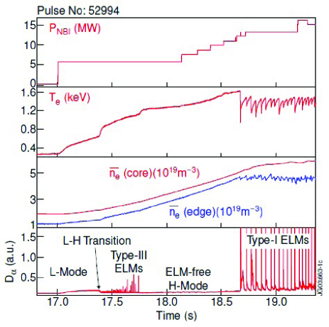
Figure 1: JET typical ELM signals ([Perez2004, thesis]).

We just focus on the signal itself and ignore all the other information behind, i.e., we just discuss how to use (as simple as possible) equations or other approaches to reproduce the shape of these signals. It is qualitative or at most semi-quantitative.

II Ordinary Differential Equation (ODE)

This is a wide used approach for modeling. For example, the famous prey-predator model for fishbone and drift wave-zonal flow system. One may also extend it to PDE to contain the spatial information. Indeed, this way has been used to model ELM and L-H transit in literatures, e.g., [Diamond1994], [Itoh1991, 1993, 1999].

If we assume that the dynamic of signal is not explicit depend on time $t$, then one equation $\dot{y}=f(y)$ is not enough because that $\dot{y}$ is not single valued with $y$. So, at least, we must use second order equation or use two first order equations. While, one second order equation is just a special case of two first order equations.

II.1 Example 1

In this example, we use the second option, i.e., two first order equations, which is also used in [Diamond1994]. The equations are

$${{\dot{y}}_{1}}={a_{1}}{y_{1}}-{b_{1}}y_{1}^{2}-{b_{2}}{y_{1}}{y_{2}},$$ (1)

$${{\dot{y}}_{2}}=-{a_{2}}{y_{2}}+{b_{3}}{y_{1}}{y_{2}}.$$ (2)

A result is shown in FIG. 2.

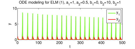
Figure 2: ODE for modeling ELM, example 1.

The physical explanations of the equations and parameters can be found in [Diamond1994], however, where $y_{1}=E$, $y_{2}=U$.

II.2 Example 2

Using one second order equation, e.g.,

$$\ddot{y}=a(1-b{y^{2}})(\dot{y}+c)-y-ac,$$ (3)

which is modified from stiff system equation, a result is shown in FIG. 3.

The shape is very similar to the PDE result in [Itoh1993]. But, an apparent drawback of (3) is that the signal $y$ is not always positive here.

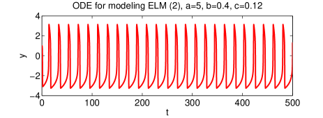
Figure 3: ODE for modeling ELM, example 2.

III Delay Differential Equation (DDE)

DDEs contain derivatives which depend on previous time. We guess some equations here. The equations are from or modified from [Shampine2000]. There is also a type of DDE has sawtooth solutions (see e.g., [Mallet-Paret2011]), which may be also suitable for model the unsolved sawteeth phenomena in magnetic confined fusion study.

III.1 Example 1

The equation is

$$y^{\prime}(t)=-\lambda y(t-1)(1+y(t)),$$ (4)

$$y(t)=t,t\leq 0.$$ (5)

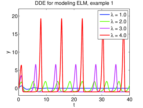
Figure 4: DDE for modeling ELM, example 1.

Results are shown in FIG. 4.

III.2 Example 2

Equation is

$$y^{\prime}(t)=ry(t)\left({1-{{y\left({t-0.74}\right)}\over m}}\right),$$ (6)

$$y(t)=19,t<0;y(0)=19.001.$$ (7)

which is original to model four-year cycle of the population of lemmings.

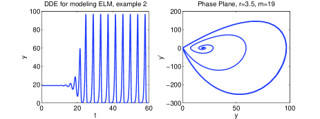
Figure 5: DDE for modeling ELM, example 2.

The result is shown in FIG. 5.

IV Differential Equation + Monte Carlo (DEMC)

This is a more intuitive way to model ELM, which combines different time scales using a more acceptable approach. The burst of ELM signal is suggested related to peeling-ballooning mode in standard ELM model ([Connor1998]). So, we give two time scale: transport time scale and ballooning mode time scale.

To simplify the transport process, the transport time scale is modeled using

$${d\over{dt}}f(t)={f\over{{\tau_{T}}}}.$$ (8)

When pressure gradient exceeds marginal value (using $f_{c1}$ to represent it), the ballooning mode occurs. The signals will grow exponentially

$${d\over{dt}}f(t)={\gamma_{BM}}f,$$ (9)

with the characteristic time $\tau_{BM}=1/\gamma_{BM}$.

When $f(t)$ exceeds a marginal value $f_{c2}$, the plasma crash. And then, go to next cycle. We also add some randomicities to $f_{c1}$ and $f_{c2}$ to make the whole signal more like the actual experimental signal. A result is shown in FIG. 6.

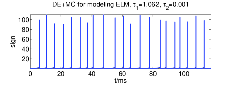
Figure 6: DEMC modeling for ELM.

This simple DEMC model captures some fundamental properties of integrated simulations, such as [Chang2008] and [Lonnroth2009].

V Summary and More

Which one is more reasonable? At present, I choose DEMC $>$ ODE $>$ DDE. While, maybe none of them can be final explanation of ELM or H-mode.

There is another math tool called Fractional Differential Equation (FDE), which has been used for anomalous transport/diffusion problems in some areas. For plasma community, FDE is not wide accepted yet, but it is possible in the future. FDE is hard to give periodic solutions as ELM at present. So, I haven’t given examples.

References

- (1) Chang, C. S.; Klasky, S.; Cummings, J.; Samtaney, R.; Shoshani, A.; Sugiyama, L.; Keyes, D.; Ku, S.; Park, G.; Parker, S.; Podhorszki, N.; Strauss, H.; Abbasi, H.; Adams, M.; Barreto, R.; Bateman, G.; Bennett, K.; Chen, Y.; Azevedo, E. D.; Docan, C.; Ethier, S.; Feibush, E.; Greengard, L.; Hahm, T.; Hinton, F.; Jin, C.; Khan, A.; Kritz, A.; Krsti, P.; Lao, T.; Lee, W.; Lin, Z.; Lofstead, J.; Mouallem, P.; Nagappan, M.; Pankin, A.; Parashar, M.; Pindzola, M.; Reinhold, C.; Schultz, D.; Schwan, K.; Silver, D.; Sim, A.; Stotler, D.; Vouk, M.; Wolf, M.; Weitzner, H.; Worley, P.; Xiao, Y.; Yoon, E. and Zorin, D., Toward a first-principles integrated simulation of tokamak edge plasmas, Journal of Physics: Conference Series, 2008, 125, 012042.
- (2) Connor, J. W.; Hastie, R. J.; Wilson, H. R. and Miller, R. L., Magnetohydrodynamic stability of tokamak edge plasmas, Physics of Plasmas, 1998, 5, 2687-2700.
- (3) Diamond, P. H.; Liang, Y.-M.; Carreras, B. A. and Terry, P. W., Self-Regulating Shear Flow Turbulence: A Paradigm for the L to H Transition, Phys. Rev. Lett., 1994, 72, 2565-2568.
- (4) Itoh, S.-I.; Itoh, K.; Fukuyama, A. and Miura, Y., Edge localized mode activity as a limit cycle in tokamak plasmas, Phys. Rev. Lett., 1991, 67, 2485-2488.
- (5) Itoh, S.-I.; Itoh, K. and Fukuyama, A., The ELMy H mode as a limit cycle and the transient responses of H modes in tokamaks, Nuclear Fusion, 1993, 33, 1445.
- (6) Itoh, K.; Itoh, S. I. and Fukuyama, A., Transport and Structural Formation in Plasmas, IOP, 1999.
- (7) Lonnroth, J.-S., A Predictive Modelling of Edge Transport Phenomena in ELMy H-Mode Tokamak Fusion Plasmas, Helsinki University of Technology, PhD thesis, 2009.
- (8) Mallet-Paret, J. and Nussbaum, R. D., Superstability and rigorous asymptotics in singularly perturbed state-dependent delay-differential equations, Journal of Differential Equations, 2011, 250, 4037 - 4084.
- (9) Perez, C., MHD analysis of edge instabilities in the JET tokamak, University of Utrecht, PhD thesis, 2004.
- (10) L. F. Shampine, Solving Delay Differential Equations with dde23, Mathematics Department Southern Methodist University, 2000.