MESA MODELS OF CLASSICAL NOVA OUTBURSTS:
THE MULTICYCLE EVOLUTION AND EFFECTS OF CONVECTIVE BOUNDARY MIXING

Abstract

Novae are cataclysmic variables driven by accretion of H-rich material onto a white-dwarf (WD) star from its low-mass main-sequence binary companion. New time-domain observational capabilities, such as the Palomar Transient Factory and Pan-STARRS, have revealed a diversity of their behaviour that should be theoretically addressed. Nova outbursts depend sensitively on nuclear physics data, and more readily available nova simulations are needed in order to effectively prioritize experimental effort in nuclear astrophysics. In this paper we use the MESA stellar evolution code to construct multicycle nova evolution sequences with CO WD cores. We explore a range of WD masses and accretion rates as well as the effect of different cooling times before the onset of accretion. In addition, we study the dependence on the elemental abundance distribution of accreted material and convective boundary mixing at the core-envelope interface. Models with such convective boundary mixing display an enrichment of the accreted envelope with C and O from the underlying white dwarf that is commensurate with observations. We compare our results with the previous work and investigate a new scenario for novae with the ³He-triggered convection.

1 Introduction

Classical novae are the result of thermonuclear explosions of H-rich material occurring on the surfaces of white dwarfs (WDs). Such events typically occur in a close binary system containing a cold WD primary component and a low-mass main-sequence (MS) star, the latter filling its Roche lobe (José & Hernanz, 2007a; Gehrz et al., 1998). The solar-composition material from the envelope of the secondary component streams through the inner Lagrangian point to form an accretion disk and eventually, after having lost its orbital angular momentum, joins the WD. For sufficiently low accretion rates ($\dot{M}\approx 10^{-11}$ – $10^{-9}\,M_{\odot}/\mbox{yr}$), the accreted material accumulates in a thin layer atop the WD until its base temperature, that rises because of gravitational compression, reaches a value at which H begins to burn, initially in the pp-chain reactions and then in the CNO cycle. As a result, a thermonuclear runaway (TNR) ensues causing rapid increases in both the temperature and energy output. Peak temperatures during classical nova outbursts can be as high as $T_{\rm max}=2-4\times 10^{8}\,\mathrm{K}$, approaching the virial temperature. Under such conditions, the proton-capture reactions of the CNO cycle become so fast that they build up large amounts of $\beta^{+}$-unstable isotopes of N, O, and F. Their temperature-independent decay rates then limit the energy generation in the CNO-cycle (Starrfield, Truran, & Sparks 1978). For neon novae, the activation of the NeNa and MgAl cycles driven by injection of Ne-seed nuclei from the ONe-rich substrate can lead to nuclear processing of even higher mass isotopes. After a time period of $10^{2}-10^{3}$ seconds, the electron-degenerate conditions are lifted as the hot convective envelope expands. Mass loss ensues either from a wind or Roche lobe overflow triggered by the radius expansion of the burning WD.

Despite much progress over the past decades (e.g. José & Hernanz 2007a), some key aspects of classical novae are still poorly understood. An important one is the mixing between the accreted envelope and WD, which is required to explain the enrichment observed in most nova ejecta in heavy elements, such as C, N, O, and Ne. These can reach combined total ejected mass fractions of 30 – 40% (e.g., Gehrz et al. 1998). The TNR peak temperatures and durations do not allow for fuelling production, so the only possible explanation of this enrichment is that it originates from the underlying CO or ONe WDs. The proposed mixing models can be divided into two groups. Either it is assumed that the envelope and WD get mixed in a thin layer close to their interface before the TNR ensues (e.g., Prialnik & Kovetz 1984; MacDonald 1983; Alexakis et al. 2004), or mixing is assumed to be the result of hydrodynamic boundary mixing at the bottom of the convection zone triggered by the TNR itself (e.g., Glasner, & Livne 1995; Glasner, Livne, & Truran 1997, 2005, 2007; Casanova et al. 2010, 2011a, 2011b).

The mechanism of mass loss by novae is also not fully understood. Apparently, a supersonic outflow, a wind driven by the super-Eddington luminosity (Kato & Hachisu 1994), and an expansion of nova ejecta as a result of its common-envelope interaction with the companion star (e.g., Livio et al. 1990) all contribute to the mass ejection. Finally, there are a few key nuclear reactions relevant for nova nucleosynthesis whose rates still remain uncertain, e.g. ¹⁸F(p,$\alpha$), ²⁵Al(p,$\gamma$), and ³⁰P(p,$\gamma$), according to José & Hernanz (2007a).

Nova outbursts are recurrent events, where depending on the parameters of a particular system, $10^{3}$ – $10^{4}$ H-shell flashes would occur in a single binary system. However, most computer simulations of nova follow only an individual outburst. An exception are the models by the Tel Aviv group (Prialnik & Kovetz, 1995; Yaron et al., 2005; Epelstain et al., 2007), who followed more than 1000 flashes. They adopted mixing of the first type mentioned above, i.e.  diffusive interface mixing during quiet accretion phases between consecutive outbursts.

In this paper we address and investigate some of these issues. We describe the simulation assumptions in Section 2. As a start, we have constructed a grid of multicycle simulations of CO novae with the masses $0.65\,M_{\odot}$, $0.85\,M_{\odot}$, $1.0\,M_{\odot}$, $1.15\,M_{\odot}$, and $1.2\,M_{\odot}$ that accrete the solar-composition and CO-enriched material at rates $\dot{M}=10^{-11}$, $10^{-10}$, and $10^{-9}\,M_{\odot}/\mbox{yr}$ (Section 3). The exact value of the WD mass dividing CO and ONe novae is not well settled. Current estimates suggest a value of about $1.1\,M_{\odot}$ when the effect of binarity is taken into account(Gil-Pons et al., 2003). As a verification exercise, we confirm the result obtained by Glasner & Truran (2009) that, for massive and slowly accreting CO WDs, the peak temperature achieved during the TNR becomes a much steeper function of WD’s central temperature, when the latter is lower than $10^{7}\,\mathrm{K}$ (Section 4). We then investigate, for the $1.2\,M_{\odot}$ case, the effect of convective boundary mixing (CBM) during the TNR (Section 5.1). For these simulations we invoke an exponentially decaying mixing efficiency model that has already been studied previously in related stellar evolution phases, such as the He-shell flash convection zones in AGB stars (e.g. Herwig et al., 1999). Finally, we report on a new scenario for novae with the ³He-triggered convection (Section 5.2), and give conclusions in Section 6.

2 Simulation Assumptions

The calculations are performed with the stellar evolution code Modules for Experiments in Stellar Evolution (MESA, Paxton et al., 2011), [rev. 3611]. From the available options we use the 2005 update of the OPAL EOS tables (Rogers & Nayfonov 2002) supplemented for lower temperatures and densities by the SCVH EOS that includes partial dissociation and ionization caused by pressure and temperature (Saumon, Chabrier, & van Horn 1995). Additionally, the HELM (Timmes & Swesty 2000) and PC (Potekhin & Chabrier 2010) EOSs are used to cover the regions where the first two EOSs are not applicable. In particular, the HELM EOS takes into account electron-positron pairs at high temperature, while the PC EOS incorporates crystallization at low temperature. Both assume complete ionization. There are smooth transitions between the four EOS tables. When creating WD models and following their subsequent nova evolution, different parts of our computed stellar models are entering the $\rho$ – $T$ domains covered by all of the above EOSs. We use the OPAL opacities (Iglesias & Rogers 1993, 1996) supplemented by the low $T$ opacities of Ferguson et al. (2005), and by the electron conduction opacities of Cassisi et al. (2007) (for details, see Paxton et al. 2011).

As in any other phase of stellar evolution, the adopted nuclear network has to be as large as necessary in order to account for the energy generation, yet as small as possible in order to make computations not too expensive. In MESA, we use the option to solve the nuclear reaction network, the structure equation and mixing operators simultaneously. This leads to a more stable numerical behaviour, however it makes adding species to the nuclear network relatively more expensive compared to using a nuclear reaction operator split option.

We have started our CO nova simulations with 77 isotopes from H to ⁴⁰Ca coupled by 442 reactions and then gradually reduced these numbers checking that this does not lead to noticeable changes in the time variation of the peak temperature. As a result, an acceptable compromise has been found empirically, and the following 33 isotopes were selected: ¹H, ³He, ⁴He, ⁷Li, ⁷Be, ⁸B, ¹¹B, ¹²C, ¹³C, ¹³N, ¹⁴N, ¹⁵N, ¹⁴O, ¹⁵O, ¹⁶O, ¹⁷O, ¹⁸O, ¹⁷F, ¹⁸F, ¹⁹F, ¹⁸Ne, ¹⁹Ne, ²⁰Ne, ²¹Ne, ²²Ne, ²¹Na, ²²Na, ²³Na, ²²Mg, ²³Mg, ²⁴Mg, ²⁵Mg, and ²⁶Mg. These are coupled by 65 reactions, including those of the pp chains (the pep reaction, whose importance was emphasized by Starrfield et al. (2009), has also been added), CNO and NeNa cycles. The underlying CO WD models have been prepared using the same isotopes, while the reaction list was extended to take into account He and C burning. By default, MESA uses reaction rates from Caughlan, & Fowler (1988) and Angulo et al. (1999), with preference given to the second source (NACRE). It includes updates to the NACRE rates for ¹⁴N(p,$\gamma)^{15}$O (Imbriani et al. 2005), the triple-$\alpha$ reaction (Fynbo et al. 2005), ¹⁴N$(\alpha,\gamma)^{18}$F (Görres et al. 2000), and ¹²C$(\alpha,\gamma)^{16}$O (Kunz et al. 2002). Although the main nuclear path for a classical nova is driven by p-capture reactions and $\beta$-decays, the $\alpha$-reactions are important for establishing the chemical composition of its underlying WD. As a test, we have also tried the MESA second option for choosing the reactions rates that gives preference to the JINA REACLIB (Cyburt et al., 2010). This database has many nuclear reaction rates in common with those considered by Iliadis et al. (2010). We have not found any significant differences in our nova $T_{\rm max}(t)$ profiles between the two options, therefore we decided to stick to the default one.

The options that specify the physics and numerics assumptions of a MESA simulation are set in an inlist file. We have started from inlists of two MESA test suite cases relevant for our problem:

• make_co_wd combines some “stellar engineering” tricks into a procedure that creates CO WD models from a range of initial masses (see below),

• wd2 demonstrates the use of parameters that control accretion, as well as mass ejection options relevant for nova calculations.

Test suite case make_co_wd uses limits on the opacity during the AGB evolution to achieve rapid envelope removal without having to compute the details of many thermal pulses which eventually culminate in the so-called superwind phase. The simulation of this final tip-AGB phase of evolution is not straightforward and beyond the scope of this investigation. The procedure followed here is different from that described by Wagenhuber & Weiss (1994), but has in the end the same effect.

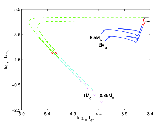
Figure 1: Generation of CO WD models with masses $0.85\,{\rm M}_{\odot}$ and $1\,{\rm M}_{\odot}$ using MESA and “stellar engineering” tricks (see text). The computations have used the $6\,{\rm M}_{\odot}$ and $8.5\,{\rm M}_{\odot}$ pre-MS stars as the initial models (the pre-MS evolution is not shown). The detailed stellar evolution computations (the solid blue curves) are followed by those in which the maximum opacity is reduced to a small value (the red curves) and the total mass of the star is relaxed to $M_{\rm WD}$ (the solid black and dashed green curves). After that, the maximum opacity is restored (the small red circles) and the WD model is given time to relax (the dot-dashed cyan curves). Finally, the WD model is cooled off to a desired temperature (the dotted magenta curves).

First, a sufficiently massive initial model has to be chosen, e.g. a $6\,M_{\odot}$ pre-MS star for the $0.85\,M_{\odot}$ WD. Its evolution is computed until the mass of its He-exhausted core reaches a value close to the final WD’s mass. This phase is shown with the solid blue curves in Fig. 1. After that, the maximum opacity is reduced to a small value (the red curves), the total mass of the star is relaxed to $M_{\rm WD}$ (the solid black and dashed green curves), the maximum opacity is restored (the small red circles), and finally the WD model is given time to relax (the dot-dashed cyan curves). As a result, the stellar model arrives at the WD cooling track, from which a WD model with a required central temperature, $T_{\rm WD}$, (a lower $T_{\rm WD}$ corresponds to a longer WD’s cooling time) can be selected (the dotted magenta curves).

In reality, a CO or an ONe WD recently formed in a binary system should be surrounded by a buffer zone of unburnt material (He-rich or CO-rich, respectively), and quite a large number of nova outbursts have to occur before it will be removed (José et al. 2003). Our WD making procedure does have a step on which the WD models possess such buffer zones. To avoid a discussion of effects to which the presence of He-rich buffer zones can lead, we remove them artificially and use naked CO WDs as the initial models for our nova simulations in this paper.

A set of the more massive CO WD models was obtained differently, by letting the $1.0\,M_{\odot}$ CO WD accrete its core composition material until the total masses of $1.15\,M_{\odot}$ and $1.2\,M_{\odot}$ were accumulated, after which the stars were cooled off to generate the massive CO WD models for a range of initial core temperature (Table 1). This special procedure has been employed because it is impossible to obtain a CO WD with $M_{\rm WD}\gtrsim 1.0\,M_{\odot}$ following the evolution of a massive AGB star, unless one artificially turns off carbon burning. For example, Gil-Pons et al. (2003) have found that for $M_{\rm ZAMS}$ increasing from $9.3\,M_{\odot}$ to $11\,M_{\odot}$ the final WD core mass for the binary star evolution is changing from $1.07\,M_{\odot}$ to $1.22\,M_{\odot}$ but, because of carbon burning in the core, it actually contains an ONe WD surrounded by a CO buffer zone, the relative mass of the latter decreasing from 7% to 0.8% for the given mass interval. Therefore, our massive CO WD models should be considered as substitutes for such ONe WDs with CO surface buffer zones. Besides, they are used for comparison with other nova simulations that involved CO WDs of similar masses.

3 MESA Models of Multicycle CO Nova Outbursts

For either CO or ONe WD the main properties of its nova outburst (such as total accreted and ejected masses, peak temperature, maximum luminosity, envelope expansion velocity, and chemical composition of the ejecta) depend mainly on the following four parameters: the WD mass $M_{\rm WD}$, its central temperature $T_{\rm WD}$ (or luminosity), the accretion rate $\dot{M}$, and the metallicity of the accreted material (e.g., Prialnik & Kovetz 1995; Townsley & Bildsten 2004; José et al. 2007). In this paper, we consider only CO WDs in binary systems with solar-metallicity companions, and in this section we ignore any mixing between the WD and its accreted envelope.

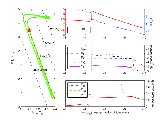
Figure 2: A snapshot of the evolution of the $1.15\,{\rm M}_{\odot}$ CO WD with $T_{\mathrm{WD}}=3\times 10^{7}\,\mathrm{K}$, accreting the solar-composition material with the rate $10^{-10}\,{\rm M}_{\odot}/\,\mathrm{yr}$. Left panel: a track in the Hertzsprung-Russell diagram for the whole nova multicycle evolution (accretion, TNR, mass loss). The star symbol shows the model internal structure of which is displayed on the right. The three right panels depict internal profiles of various stellar structure parameters as functions of the quantity $x=\log_{10}(1-q)$, where $q=M_{r}/(M_{\rm WD}+M_{\rm acc})$ is a relative mass coordinate. Here, $M_{r}$ is the mass inside a sphere of the radius $r$, while $M_{\rm acc}$ is the accreted mass. For $M_{\rm WD}\approx\,{\rm M}_{\odot}$, a value $x$ of the abscissa approximates to the decimal logarithm of solar masses located to the right of this coordinate. Upper-right: temperature (solid red) and density (dashed blue); middle-right: mass fractions of some isotopes; bottom right: adiabatic $\nabla_{\rm ad}$, radiative $\nabla_{\rm rad}$, and actual $\nabla$ temperature gradients (logarithmic and with respect to pressure, dot-dashed blue, dashed green, and solid red lines). In the convectively unstable region, $\nabla_{\rm rad}>\nabla\gtrsim\nabla_{\rm ad}$.

Fig. 2 shows a snapshot of the evolution of the hottest of our $1.15\,M_{\odot}$ CO WD models ($T_{\rm WD}\approx 3\times 10^{7}\,\mathrm{K}$; for the correspondence between the WD’s initial central temperature $T_{\rm WD}$ and luminosity $L_{\rm WD}$, see Table 1) accreting the solar-composition material with the rate $\dot{M}=10^{-10}\,M_{\odot}$/yr. The total mass $M=M_{\rm WD}+M_{\rm acc}$ increases during an accretion phase and decreases during a mass-loss event. The abrupt changes in the abundances at $x_{\rm WD}\approx-4.6$ and $x_{\rm CE}\approx-8.8$ mark the WD’s surface and upper boundary of the convective envelope, respectively. During an accretion phase, $x_{\rm WD}$ moves to the left, which signifies that the mass (of the envelope) to the right of $x_{\rm WD}$ increases; $x_{\rm WD}$ shifts to the right during a mass-loss event.

Fig. 2 corresponds to the moment, when the temperature at the interface between the WD and accreted envelope has reached its maximum value (a sharp peak on the solid red curve in the upper-right panel), and most of the initially abundant ¹²C, ¹³C, ¹⁴N, and ¹⁶O nuclei have been transformed into the $\beta^{+}$-unstable p-capture product isotopes ¹³N, ¹⁴O, ¹⁵O, and ¹⁷F (the dot-dashed blue, dashed black, dotted red and solid magenta curves in the middle-right panel) in the convective envelope (a region where $\nabla_{\rm rad}>\nabla\gtrsim\nabla_{\rm ad}$ in the lower-right panel). The $\beta$-decay times of these isotopes limit the energy production, unless additional C and O is mixed from the layers below the convection zone.

For the multicycle simulations mass loss is triggered when the models reach super-Eddington luminosities according to the following prescription:

$$\dot{M}=-2\,\eta_{\rm Edd}\,\frac{(L-L_{\rm Edd})}{v^{2}_{\rm esc}},$$ (1)

where $v_{\rm esc}=\sqrt{2GM/R}$, and $L_{\rm Edd}=(4\pi GcM)/\kappa$. Here, $M$, $R$, and $L>L_{\rm Edd}$ are the mass, radius, and luminosity of the star, while $\kappa$ is the Rosseland mean opacity at the surface. The scaling factor has been set to $\eta_{\rm Edd}=1$. This prescription simply assumes that the excess of nova luminosity over the Eddington one determines the rate of change of the mass-loss kinetic energy.

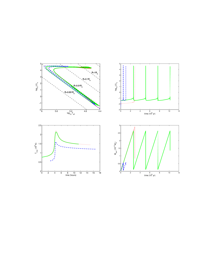
Figure 3: A comparison of three nova models that started their evolution with the CO WDs having the same mass ($M_{\rm WD}=1.15\,{\rm M}_{\odot}$) and with the same accretion rate ($\dot{M}=10^{-10}\,{\rm M}_{\odot}/\,\mathrm{yr}$). The differences in their evolution tracks (with dashed black lines of constant radius, upper-left panel), luminosity curves (upper-right panel), maximum temperatures of H burning (lower-left panel), and accreted envelope masses (lower-right panel) are caused by their different WD initial central temperatures ($T_{\rm WD}=3\times 10^{7}\,\mathrm{K}$ for the dashed blue and solid green curves, and $T_{\rm WD}=1.5\times 10^{7}\,\mathrm{K}$ for the dotted red curve) and the chemical compositions of accreted material (the solar composition for the solid green and dotted red curves, and a mixture of 70% solar and 30% CO WD compositions for the dashed blue curve).

The main results of our $1.15\,M_{\odot}$ CO nova simulations for the mass accretion rate $\dot{M}=10^{-10}\,M_{\odot}$/yr are presented in Fig. 3. Cases for accretion of solar and $30\%$ CO enriched material, as well as for different WD central temperatures are shown. The case with CO-enriched accretion material is not realistic because in the majority of actual CO novae the donor star is a Pop I MS dwarf providing material close to solar to be accreted by the WD. Therefore, the CO enrichment of nova ejecta comes from the underlying CO WDs and occurs either before or during the TNR. Nevertheless, the case with CO enhanced accretor material is frequently considered in the literature as an artificial way to mimic the effect of mixing at the core-envelope interface (e.g., José & Hernanz 1998; Starrfield et al. 1998).

The effect of the initial WD luminosity (or central temperature) on the strength of the nova explosion has been analyzed before (e.g., Starrfield et al. 1998; Yaron et al. 2005; José & Hernanz 2007b). As expected, the strongest outburst occurs in the case of the coolest WD (the dotted red curves). Its lower temperature allows the WD to accumulate a slightly more massive H-rich envelope on a longer timescale (the lower-right panel) before the TNR is triggered. This leads to a higher peak temperature, $T_{\rm max}\approx 2.29\times 10^{8}\,\mathrm{K}$, and to a longer time of envelope’s removal by the mass-loss that extends the nova evolution track towards lower effective temperatures and larger radii. The corresponding track (dotted red) reaches a maximum radius $R\approx 3\,R_{\odot}$. Evidently, to produce a self-consistent model, we should not allow the nova to expand far beyond its Roche lobe radius $R_{\rm RL}$. For example, if the $1.15\,M_{\odot}$ WD has a $0.6\,M_{\odot}$ MS companion then, for the latter to fill its Roche lobe and therefore be able to transfer its mass onto the WD, the binary rotation period has to be nearly 5 hours (for a circular orbit with a semi-major axis $a=1.8\,R_{\odot}$). In this case, the WD itself will have a Roche lobe with $R_{\rm RL}\approx 0.8\,R_{\odot}$. The MESA stellar evolution code has an option to limit the growth of a star beyond its Roche lobe radius by exponentially increasing the mass-loss rate when $R>R_{\rm RL}$, however we did not implement this option in these simulations.

The CO-enriched material ignites much earlier than the solar-composition case because it contains much larger mass fractions of CO isotopes that serve as catalysts for H burning in the CNO cycle. As a result of the lower accreted mass, the TNR peak temperature reaches only $1.59\times 10^{8}\,\mathrm{K}$ in this case (the dashed blue curves in the lower panels of Fig. 3). Table 1 summarizes the accreted masses, maximum H-burning luminosities, and peak temperatures as functions of $M_{\rm WD}$, $T_{\rm WD}$, $L_{\rm WD}$, and $\dot{M}$ obtained in the nova simulations. The number of grid zones in the envelopes of the MESA nova models varies between 500 and 1000, depending on the complexity and evolutionary phase of the model. A comparable number of grid zones is allocated to the underlying WD.

4 Comparison with Other Nova Simulations

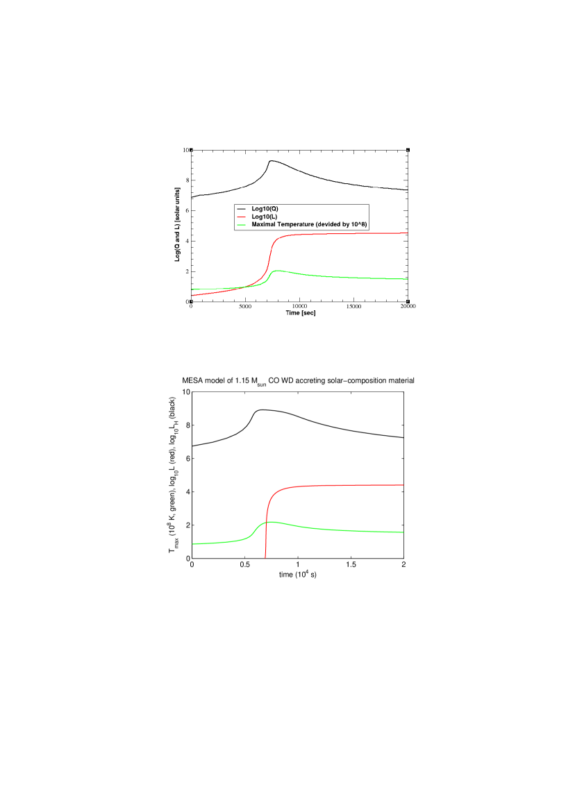
Figure 4: A comparison of the hydrogen burning luminosity ($Q$ and $L_{\rm H}$, black curves), surface luminosity ($L$, red curves), and maximum temperature (green curves) evolution profiles from Ami Glasner’s $1.147\,M_{\odot}$ (the upper panel) and our $1.15\,M_{\odot}$ (the lower panel) CO nova models accreting solar-composition material with the same rate, $\dot{M}=10^{-10}\,{\rm M}_{\odot}/\,\mathrm{yr}$. The difference in the rise of the surface luminosity is probably explained by different initial conditions and our better modeling of the evolution preceding the TNR.

Ami Glasner provided us with the parameters of his 1D model of a nova outburst occurring on a $1.147\,{\rm M}_{\odot}$ CO WD. It has a central temperature $T_{\rm WD}=2.4\times 10^{7}\,\mathrm{K}$, accretes solar-composition material at a rate $\dot{M}=10^{-10}\,{\rm M}_{\odot}/\,\mathrm{yr}$, and no interface mixing has been adopted (Glasner, Livne, & Truran, 2011). The temperature and luminosity comparison of that model with our $1.15\,M_{\odot}$ CO nova simulation with $T_{\rm WD}\approx 2.5\times 10^{7}\,\mathrm{K}$ shows very good agreement, in particular with respect to the amplitudes (Fig. 4). The relative differences between the accreted masses and peak temperatures for the two models are only 16% and 6%, respectively.

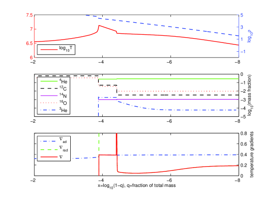
Figure 8: Same as Fig. 7, but at a later time. ³He ignition triggers a convective zone (the region where $\nabla_{\rm rad}>\nabla\gtrsim\nabla_{\rm ad}$ in the lower panel). Note the enhanced amount of C and O (middle panel) in this model with CBM, sufficient to produce a fast CO nova.

As a second test, we check if our nova model agrees with findings reported recently by Glasner & Truran (2009) that the peak temperature achieved during the TNR becomes a much steeper function of $T_{\rm WD}$ when the latter is lower than $10^{7}\,\mathrm{K}$. Their study was motivated by the result obtained earlier by Townsley & Bildsten (2004), according to which such cold WDs should be associated with nova outbursts occurring in binaries with $\dot{M}<10^{-10}\,{\rm M}_{\odot}/\,\mathrm{yr}$. To carry out this test, we let the $1.2\,{\rm M}_{\odot}$ CO WD model cool down to a central temperature $T_{\rm WD}=3.3\times 10^{6}\,\mathrm{K}$, let it accrete the solar-composition material with the rate $\dot{M}=10^{-11}\,{\rm M}_{\odot}/\,\mathrm{yr}$, and followed the ensuing nova outburst. This simulation has been complemented with the ones done for $T_{\rm WD}=7$, $15$, $20$ and $30\times 10^{6}\,\mathrm{K}$ and the same $\dot{M}$. The resulting relation between $T_{\rm max}$ and $T_{\rm WD}$ is very similar to those plotted by Glasner & Truran in their Fig. 1, and our model therefore confirm their findings. Quantitatively, for $M_{\rm WD}=1.2\,{\rm M}_{\odot}$, $T_{\rm WD}=3.3\times 10^{7}\,\mathrm{K}$, and $\dot{M}=10^{-11}\,{\rm M}_{\odot}/\,\mathrm{yr}$ our model accretes $M_{\rm acc}=1.42\times 10^{-4}\,{\rm M}_{\odot}$ envelope mass before TNR ignition and its peak temperature is $T_{\rm max}=3.28\times 10^{8}\,\mathrm{K}$, while Glasner & Truran find $M_{\rm acc}=1.30\times 10^{-4}\,{\rm M}_{\odot}$ and $T_{\rm max}=3.68\times 10^{8}\,\mathrm{K}$ for their slightly more massive WD ($M_{\rm WD}=1.25\,{\rm M}_{\odot}$) with $T_{\rm WD}=4\times 10^{7}\,\mathrm{K}$. Our data are also in a good agreement with the estimates of $M_{\rm acc}$ and $T_{\rm WD}$ presented by Townsley & Bildsten (2004) in their Fig. 8.

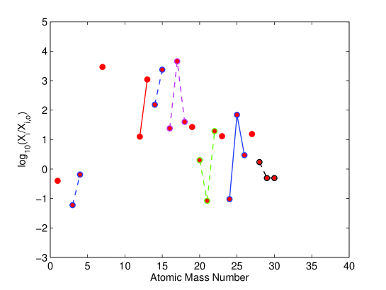
Figure 5: Solar-scaled mass-averaged abundances in the expanding envelope of a last model from our simulations of a CO nova with $M_{\rm WD}=1.15\,M_{\odot}$, $T_{\rm WD}=15\times 10^{6}$ K, and $\dot{M}=2\times 10^{-10}\,M_{\odot}/\mbox{yr}$. The accreted material was assumed to be a mixture of 50% solar and 50% WD’s core compositions. Our final abundances agree very well with those presented by José & Hernanz (1998) in their Fig. 1 for a CO nova model with similar parameters.

Finally, Fig. 5 shows solar-scaled mass-averaged abundances in the expanding envelope of a last model from our simulations of a CO nova with $M_{\rm WD}=1.15\,M_{\odot}$, $T_{\rm WD}=15\times 10^{6}$ K, and $\dot{M}=2\times 10^{-10}\,M_{\odot}/\mbox{yr}$. These simulations have used an extended nuclear network that included 48 isotopes from H to ⁴⁰Ca coupled by 120 reactions. The accreted material was assumed to be a mixture of 50% solar and 50% WD’s core compositions. This nova model has parameters similar to those of the model CO5 of José & Hernanz (1998). A comparison of our final abundances from Fig. 5 with those for the model CO5 presented by José & Hernanz (1998) in their Fig. 1 shows a very good qualitative agreement.

5 Effects of Convective Boundary Mixing

5.1 A Standard Mixing Model

The nova models presented in Section 3 do not reproduce the observed enrichment of nova ejecta in C, N, O, and other heavy elements (e.g. Gehrz et al., 1998) because they do not include the interface mixing between the accreted H-rich envelope and its underlying CO WD. Recent two- and three dimensional nuclear-hydrodynamic simulations of a nova outburst have shown that a possible mechanism of this mixing are the hydrodynamic instabilities and shear-flow turbulence induced by steep horizontal velocity gradients at the bottom of the convection zone of the TNR (Casanova et al., 2011b). These hydrodynamic processes associated with the convective boundary lead to convective boundary mixing (CBM) at the base of the accreted envelope into the outer layers of the WD. As a result, CO-rich (or ONe-rich) material is dredged-up during the TNR.

Our nova simulations have been performed with the one-dimensional stellar evolution code MESA. For one-dimensional CBM calculations, MESA provides a simple model that treats the time-dependent mixing as a diffusion process, and that approximates the rate of mixing by an exponentially decreasing function of a distance from the formal convective boundary,

$$D_{\rm OV}=D_{0}\exp\left(-\frac{2|r-r_{0}|}{fH_{P}}\right),$$ (2)

where $H_{P}$ is the pressure scale height, and $D_{0}$ is a diffusion coefficient, calculated using a mixing-length theory (MLT), that describes convective mixing at the radius $r_{0}$ close to the boundary. In this model $f$ is a free parameter that is calibrated for each type of convective boundary either semi-empirically through observations, or through multi-dimensional hydrodynamic simulations.

The MESA CBM model is based on the findings in hydrodynamic models (Freytag, Ludwig, & Steffen, 1996) that the velocity field, and along with it the mixing expressed in terms of a diffusion coefficient, decays exponentially in the stable layer adjacent to a convective boundary. Following these findings, the CBM model extends time-dependent mixing according to the MLT diffusion coefficient $D_{\mathrm{MLT}}$ across the Schwarzschild boundary with the diffusion coefficient given by Equation (2). The total diffusion coefficient is therefore $D=D_{\mathrm{MLT}}+D_{\mathrm{OV}}$. In the CBM model adopted here the energy transport in the convectively stable layer is assumed to be due to radiation only. This CBM model was first introduced in stellar evolution calculations by Herwig et al. (1997). This, or very similar models, have been applied to several related situations in stellar evolution. The most relevant, because similar, case is CBM at the bottom of the He-shell flash (or pulse-driven) convection zone (PDCZ) in AGB stars (e.g. Herwig et al., 1999; Miller Bertolami et al., 2006; Weiss & Ferguson, 2009). The consequences include larger ${}^{12}\mathrm{C}$ and ${}^{16}\mathrm{O}$ abundances in the intershell, in agreement with observations of H-deficient post-AGB stars if $f_{\mathrm{PDCZ}}\sim 0.008$ (Werner & Herwig, 2006). Multidimensional hydrodynamic simulations of He-shell flash convection seem to support this value of $f_{\mathrm{PDCZ}}$ (Herwig et al., 2006, 2007), but more sophisticated numerical hydrodynamics work is needed.

The MESA CBM model is meant to represent a wide range of hydrodynamic instabilities that may contribute to mixing at the convective boundary. The cases considered by Freytag, Ludwig, & Steffen (1996) featured shallow near-surface convection zones with a small ratio of the stability in the unstable and stable zones. These convection zones display the classical overshoot picture in which coherent convective systems cross the convective boundary and then turn around due to buoyancy effects. The boundaries of shell-flash convection, such as those in novae or in AGB stars, are much stiffer, and coherent convective blobs cannot cross the convective boundary. Instead, shear motion, induced by convective flows and internal gravity waves lead to mixing at the convective boundaries in which the Kelvin-Helmholtz instability plays an important role (Herwig et al., 2006; Casanova et al., 2011b). The amount of CBM, as expressed in the free parameter $f$, depends on the details of the specific conditions, including the relative stability of the stable to unstable side of the boundary as well as the vigour of the convection. While for shallow surface convection $f$ was found to be in the range $0.25\dots 1.0$, hydrodynamic and semi-empirical studies show that $f=0.008$ is appropriate for the bottom of the He-shell flash convection zone.

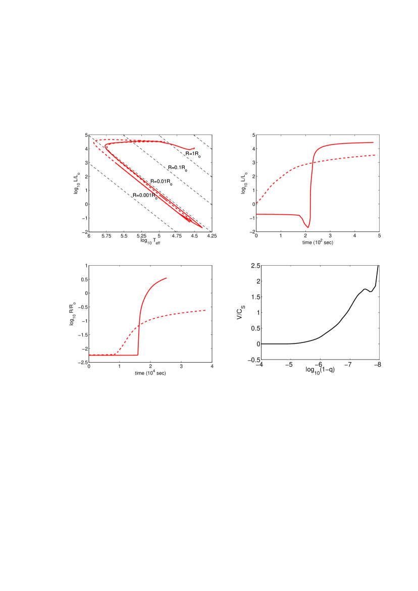
Figure 6: Results of the $1.2\,M_{\odot}$ CO nova simulation with convective boundary mixing according to Equation 2 (solid red curves). Upper-left panel: HRD; upper-right and lower-left panels: very fast increase of the surface luminosity and a bit slower radial expansion; lower-right panel: velocity profile (in the units of the sound speed) in one of the last models. For comparison, the dashed red curves show the results for the same model but without CBM.

For the nova simulations we adopt $f_{\mathrm{nova}}=0.004$ at the bottom of the TNR convective zone, that eventually includes most of the accreted envelope. This number is of the same order of magnitude (within a factor of two) compared to CBM efficiencies that have been found to reproduce observables related to the He-shell flash convection zone in AGB stars. As a result, ¹²C and ¹⁶O are mixed from the WD below, and their combined mass fraction in the convective zone reaches $Z_{\rm CO}\approx 0.29$. Such a CO abundance is similar to the average mass fraction of CNO elements observed in the ejecta of CO novae. With this increase in the total CO abundance, the simulation produces a fast CO nova. The surface (bolometric) luminosity increases by six orders of magnitude on a timescale of 50 seconds (the solid red curve in the upper-right panel in Fig. 6). The radius increases on a longer timescale, of the order of $10^{4}$ seconds (the lower-left panel). This corresponds to a surface expansion velocity of nearly 300 km/s. The velocity exceeds the speed of sound only in the outer layers of the expanding envelope, which has a negligible relative mass (the lower-right panel). Given the very short evolution timescale of this nova model, its post-TNR mass-loss cannot anymore be caused by the super-Eddington luminosity alone because the associated mass-loss rate (1) is too slow. Instead, the envelope would rather quickly fill the WD’s Roche lobe, after which it would probably be expelled from the binary system as a result of its (common-envelope) interaction with the secondary component (e.g., Livio et al. 1990). The details of this process are not yet understood, and we do therefore not attempt multicycle simulations of nova models with CBM.

As an additional test, we compare the maximum hydrogen-burning luminosities $L_{\rm H}$ achieved in the basic $1.2\,{\rm M}_{\odot}$ CO nova models with simple estimates based on the approximation of the nuclear energy generation rate limited by the mass fraction of CNO elements $Z_{\rm CNO}$ in the convective envelope of a CO nova during its TNR. When limited by the $\beta$ decays (e.g. “Hot” CNO cycle),

$$\varepsilon_{\rm max}\approx 5.6\times 10^{13}\left(\frac{Z_{\rm CNO}}{0.01}\right)\ \ \ \mbox{erg}\cdot\mbox{g}^{-1}\cdot\mbox{s}^{-1},$$

(Glasner, Livne, & Truran, 2007), and given that $L_{\rm H}\approx\varepsilon_{\rm max}M_{\rm conv}$, where $M_{\rm conv}$ is the mass of the convective envelope, the hydrogen-burning luminosity can be estimated as:

$$\log_{10}\frac{L_{\rm H}}{L_{\odot}}\approx 8.48+\log_{10}\frac{Z_{\rm CNO}}{0.01}+\log_{10}\frac{M_{\rm conv}}{10^{-5}\,{\rm M}_{\odot}}.$$ (3)

Without any CBM the CNO abundance is $Z_{\rm CNO}=Z_{\odot}=0.019$ and $M_{\rm conv}\approx M_{\rm acc}=1.9\times 10^{-5}\,{\rm M}_{\odot}$ (data from Table 1 for $M_{\rm WD}=1.2\,{\rm M}_{\odot}$, $T_{\rm WD}=3.0\times 10^{7}\,\mathrm{K}$, and $\dot{M}=10^{-10}\,{\rm M}_{\odot}/\,\mathrm{yr}$), in which case the equation (3) estimates $\log_{10}(L_{\rm H}/L_{\odot})\approx 9.04$, while our numerical simulations give 8.74. In models with CBM the mass of the convective envelope $M_{\rm conv}\approx 4.2\times 10^{-5}\,{\rm M}_{\odot}$ exceeds the accreted mass by the amount of material dredged up from the WD core. In this case, $Z_{\rm CNO}\approx Z_{\rm CO}\approx 0.29$, which results in $\log_{10}(L_{\rm H}/L_{\odot})=10.56$. The numerical simulations give $\log_{10}(L_{\rm H}/L_{\odot})=10.67$. The maximum H-burning temperature reached during the outburst of our mixed CO nova is $2.32\times 10^{8}\,\mathrm{K}$ which is $7\times 10^{6}\,\mathrm{K}$ higher than $T_{\rm max}$ in the corresponding unmixed model.

5.2 Mixing Caused by ³He Burning

Shen & Bildsten (2009) have quantified the role of ³He in the onset of a nova. They have shown that if the mass fraction of ³He in the H-rich material accreted onto a WD is higher than $X(^{3}\mbox{He})=2\times 10^{-3}$ then convection in the nova envelope is triggered by the ³He(³He,2p)⁴He reaction, rather than by ¹²C(p,$\gamma)^{13}$N. This alters the amount of mass that is accreted prior to a nova outburst and should therefore be taken into account when comparing the observed and theoretically predicted nova rates. As a likely place for novae with the ³He-triggered convection, Shen & Bildsten (2009) consider binaries in which a low-mass MS component has undergone such significant mass-loss that it now exposes its formerly deep layers where ³He was produced in a large amount as a result of incomplete pp-chain reactions (the so-called “³He bump”).

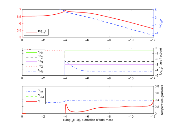
Figure 7: Snapshot similar to Fig. 2 for a $1.2\,M_{\odot}$ CO WD model with the central temperature $T_{\rm WD}=3.3\times 10^{6}\,\mathrm{K}$ that accretes with the rate $\dot{M}=10^{-11}\,{\rm M}_{\odot}/\,\mathrm{yr}$. Note formation of a sloped ³He enhancement at the base of the accreted envelope (the dot-dashed blue curve in the middle panel) during the accretion. The envelope is convectively stable yet, therefore $\nabla$ coincides with $\nabla_{\rm rad}$ everywhere (the lower panel).

In our simulations, we have found a variation of this ³He-triggered convection scenario, i.e. that the nova can generate the ³He in situ. The new scenario is based on the results obtained by Townsley & Bildsten (2004), who have demonstrated that WDs accreting with rates $\dot{M}<10^{-10}\,{\rm M}_{\odot}/\,\mathrm{yr}$ should maintain their central temperatures at the level of $T_{\rm WD}<10^{7}\,\mathrm{K}$. We have presented such a CO WD model with $M_{\rm WD}=1.2\,{\rm M}_{\odot}$, $T_{\rm WD}=3.3\times 10^{6}\,\mathrm{K}$ and $\dot{M}=10^{-11}\,{\rm M}_{\odot}/\,\mathrm{yr}$ in Section 4. In this model a large amount of ³He, $X(^{3}\mbox{He})\approx 5\times 10^{-3}$, is produced at the base of the accreted envelope (the dot-dashed blue curve in the middle panel in Fig. 7). The “sloped ³He enhancement” is formed as a result of incomplete pp-chain reactions, like the ³He bump in low-mass MS stars. Eventually, ³He ignition triggers convection, as predicted by Shen & Bildsten (2009). When we include CBM in this model, as we did for the standard mixing model using $f_{\mathrm{nova}}=0.004$ in the equation (2), the ³He-driven convection penetrates into the WD’s outer layers and dredges up large amounts of C and O into the convective envelope (the middle panel in Fig. 8), allowing subsequently for a fast nova. Note that this interface mixing occurs before the TNR, when the maximum temperature is still lower than $5\times 10^{7}\,\mathrm{K}$. It is not until the ³He abundance in the convective zone decreases below its solar value that the major TNR driven by H-burning in the CNO cycle will ensue.

A comparison of the time intervals between successive nova outbursts (the accretion times), $t_{\rm acc}=M_{\rm acc}/\dot{M}$, that can be estimated using the corresponding numbers from Table 1, for the $1.2\,M_{\odot}$ models with $T_{\rm WD}=20\times 10^{6}$ K and $T_{\rm WD}=3.3\times 10^{6}$ K, and with the accretion rates $10^{-10}\,M_{\odot}/\mbox{yr}$ and $10^{-11}\,M_{\odot}/\mbox{yr}$, respectively, shows that for one event involving the cold and slowly accreting WD there should be nearly 59 events occurring on the hot and faster accreting WD, provided that the both types of cataclysmic variables are already present in equal amounts. Given that the last assumption is not true, because the cooling time for the second model is much longer than that for the first one, the relative observational frequency of novae with the ³He-triggered convection should actually be very low. We plan to study nova models with the ³He-triggered convection in more detail, even though as a purely theoretical case, in our future work.

6 Conclusion

We have presented a grid of nova simulations with the one-dimensional stellar evolution code MESA, and provided some tests and comparison with works by others, to demonstrate that MESA can generate state-of-the-art nova simulations. In addition, we have investigated the effect of convective boundary mixing at the bottom of the TNR convection zone. Interestingly, the CBM efficiency that reproduces observed CO enhancements is of the same order of magnitude (within a factor two) compared to CBM efficiencies that have been found to reproduce observables related to the He-shell flash convection zone in AGB stars. We do not consider this a coincidence, but rather it is likely that in both cases very similar physics of CBM is at play, namely shear motion of convective flows and internal gravity waves leading to mixing at the convective boundary, in which the Kelvin-Helmholtz instability plays an important role. It will be exciting to study both phenomena side by side in the future. For example, the one-dimensional simulations performed here are related to the results of multi-dimensional simulations of CBM reported by Herwig et al. (2007). The CBM mixing parameter $f_{\mathrm{nova}}=0.004$ turns out to be sufficient to reproduce both the observed heavy-element enrichment of CO novae, as well as amounts of CO-rich material dredged up in numerical simulations of the Kelvin-Helmholtz and other hydrodynamic instabilities in the novae case (e.g., Casanova et al. 2010, 2011a, 2011b).

Further, we have studied slow accretion of solar-composition material onto a CO WD with the central temperature $T_{\rm WD}=3.3\times 10^{6}\,\mathrm{K}$, exploring the original scenario proposed by Townsley & Bildsten (2004) in which nova outbursts can actually occur under such conditions. We have found that incomplete pp-chain reactions lead to the formation of a sloped ³He enhancement at the base of the accreted envelope in this case, with the maximum mass fraction $X(^{3}\mbox{He})\approx 5\times 10^{-3}$. As predicted by Shen & Bildsten (2009) for this high abundance, ³He ignites before the major TNR, and this triggers the development of a convective zone adjacent to the WD’s surface. When complemented with CBM mixing, sufficiently large amounts of C and O are mixed into the envelope to produce a fast CO nova. These new results may suggest a more probable scenario, as compared to the one proposed by Shen & Bildsten (2009), for the ³He-triggered novae. Clearly this aspect of the nova evolution deserves further investigation, in spite of the fact that the relative observational frequency of novae with the ³He-triggered convection is expected to be very low.

Table 1: Characteristics of Our CO Nova Models

$M_{\rm WD}[\,{\rm M}_{\odot}]$	$T_{\rm WD}[10^{6}\,\mathrm{K}]$	$\lg\,L_{WD}[\mathrm{L_{\odot}}]$	$\lg\,\dot{M}[\,{\rm M}_{\odot}$/yr]	$M_{\rm acc}$ [$10^{-5}\,{\rm M}_{\odot}$]	$\lg\,L_{\mathrm{H}}[\mathrm{L_{\odot}}]$	$T_{\rm max}[10^{6}\,\mathrm{K}]$
0.65	30	-1.65	-9	22.0	8.06	127
0.65	30	-1.65	-10	22.5	8.10	126
0.65	30	-1.65	-11	22.7	8.14	129
0.85	15	-2.35	-9	9.8	8.58	154
0.85	15	-2.35	-10	12.2	9.05	165
0.85	15	-2.35	-11	11.9	9.03	164
1.0	30	-1.55	-9	5.3	8.96	181
1.0	30	-1.55	-10	5.8	9.03	184
1.0	30	-1.55	-11	5.7	9.02	184
1.15	30	-1.50	-10	2.6	8.87	213
1.15	30	-1.50	-10	0.6	8.63	159
1.15	30	-1.50	-10	2.6	10.67	222
1.15	25	-1.70	-10	2.9	8.92	218
1.15	20	-1.94	-10	3.2	8.97	223
1.15	15	-2.25	-10	3.6	9.03	229
1.15	12	-2.50	-10	3.5	8.95	222
1.15	10	-2.69	-10	4.1	9.08	234
1.15	7	-3.07	-10	5.8	9.26	249
1.15	7	-3.07	-11	5.2	9.42	244
1.2	30	-1.49	-9	1.6	8.68	220
1.2	30	-1.49	-10	1.9	8.74	225
1.2	30	-1.49	-10	0.3	8.47	156
1.2	30	-1.49	-10	1.9	10.67	232
1.2	30	-1.49	-11	1.8	8.74	225
1.2	20	-1.92	-9	1.4	8.62	215
1.2	20	-1.92	-10	2.4	8.86	237
1.2	20	-1.92	-11	2.3	8.85	238
1.2	15	-2.23	-9	1.8	8.68	221
1.2	15	-2.23	-10	2.2	8.76	228
1.2	15	-2.23	-11	2.7	8.92	242
1.2	7	-3.04	-11	4.0	9.14	261
1.2	3.3	-3.74	-11	14.2	9.70	328

References

- Alexakis et al. (2004) Alexakis, A., Calder, A. C., Heger, A., Brown, E. F., Dursi, L. J., Truran, J. W., Rosner, R., Lamb, D. Q., Timmes, F. X., Fryxell, B., Zingale, M., Ricker, P. M., & Olson, K. 2004, ApJ, 602, 931
- Angulo et al. (1999) Angulo, C., et al. 1999, Nucl. Phys. A, 656, 3
- Casanova et al. (2010) Casanova, J., José, J., García-Berro, E., Calder, A., & Shore, S. N. 2010, A&A, 513, L5
- Casanova et al. (2011a) Casanova, J., José, J., García-Berro, E., Calder, A., & Shore, S. N. 2011a, A&A, 527, A5
- Casanova et al. (2011b) Casanova, J., José, J., García-Berro, E., Shore, S. N., & Calder, A. 2011b, Nature, 478, 490
- Cassisi et al. (2007) Cassisi, S., Potekhin, A. Y., Pietrinferni, A., Catelan, M., & Salaris, M. 2007, ApJ, 661, 1094
- Caughlan, & Fowler (1988) Cauglan, G. R., & Fowler, W. A. 1988, At. Data Nucl. Data Tables, 40, 283
- Cyburt et al. (2010) Cyburt, R. H., Amthor, A. M., Ferguson, R., Meisel, Z., Smith, K., Warren, S., Heger, A., Hoffman, R. D., Rauscher, T., Sakharuk, A., Schatz, H., Thielemann, F. K., & Wiescher, M. 2010, ApJS, 189, 240
- Epelstain et al. (2007) Epelstain, N., Yaron, O., Kovetz, A., & Prialnik, D. 2007, MNRAS, 374, 1449
- Ferguson et al. (2005) Ferguson, J. W., Alexander, D. R., Allard, F., Barman, T., Bodnarik, J. G., Hauschildt, P. H., Heffner-Wong, A., & Tamanai, A. 2005, ApJ, 623, 585
- Freytag, Ludwig, & Steffen (1996) Freytag, B., Ludwig, H.-G., & Steffen, M. 1996, A&A, 313, 497
- Fynbo et al. (2005) Fynbo, H. O. U., et al. 2005, Nature, 433, 136
- Gehrz et al. (1998) Gehrz, R. D., Truran, J. W., Williams, R. E., & Starrfield, S. 1998, PASP, 110, 3
- Gil-Pons et al. (2003) Gil-Pons, P., García-Berro, E., José, J., Hernanz, M., & Truran, J. W. 2003, A&A, 407, 1021
- Glasner, & Livne (1995) Glasner, S. A., & Livne, E. 1995, ApJ, 445, L149
- Glasner, Livne, & Truran (1997) Glasner, S. A., Livne, E., & Truran, J. W. 1997, ApJ, 475, 754