Presence of anisotropic pressures in Lemaître-Tolman-Bondi cosmological models

Abstract

We describe Lemaître-Tolman-Bondi cosmological models where an anisotropic pressures is considered. By using recent astronomical observations coming from supernova of Ia types we constraint the values of the parameters that characterize our models.

I Introduction

About a decade ago, current local measurements of redshift and luminosity-distance relations of Type Ia Supernovae (SNIa)S10 indicate that the expansion of the universe presents an accelerated phase R98 ; P99 . In fact, the astronomical measurements showed that the SNe at a redshift of $z\sim 0.5$ were systematically fainted, which could be attributed to an acceleration of the universe. These local observations can then be extrapolated to the universe at large, and the resulting Friedmann-Robertson-Walker (FRW) model can be used to interpret all cosmological measurements, which strongly support a dominant dark energy component, responsible for this cosmological acceleration.

It is usual to say that this accelerated expansion is due to a cosmological constant, the so called concordance $\Lambda$CDM, which fits the observations quite well, but there is no theoretical understanding of the origin of this cosmological constant or its magnitude (the well known cosmological constant problem). Also, this model presents a coincidence problem of late cosmic acceleration, which establishes the fact that the density values of dark matter and dark energy are of the same order precisely todaydCHP2008 .

In order to get rid of the above problems there has been put forward other kind of different models, where some exotic, unknown and uncluttered matter component, dubbed dark energyHT99 (see also Refs. T10 ; C09 for recent reviews) is considered. Among these possibilities are quintessence C98 ; Z98 , k-essence Ch00 ; AP00 ; AP01 , phantom field C02 ; C03 ; H04 , holographic dark energy Z07 ; W07 ; julio , etc. (see Ref. D09 for model-independent description of the properties of the dark energy and Ref. S09 for possible alternatives). However, although fundamental for our understanding of the evolution of the universe, the nature of this quintessence remains a completely open question nowadays, moreover, very often they require fine-tuningCST06 ; S06 .

All these models work under the assumption of the Cosmological Principle, which imposes homogeneity and isotropy. But, the question is, are these symmetries consistent with observations? We know that inhomogeneities are abundant in the universe: there are not only clusters of galaxies but also large voids. It has usually been argued that these symmetries should only be valid on very large scales.

It is true that this recognition is a result of the strict use of a FRW homogeneous and isotropic model. However, inhomogeneous models have been put forward. For instance, if phantom energy is considered, then it is possible to sustain traversable wormholes in which the phantom matter is an inhomogeneous and anisotropic fluidCLdCCS08 ; CdCMS09 ; CdC12 . Also, the authors of Ref. GGMP considered inhomogeneous metrics, but with an equation of state given by $P=\omega\rho$, with $\omega$ the equation of state parameter being constant. Here, they study the gravitational collapse of spherical symmetric physical systems. On the same line of reasoning, the author of Ref. LL06 studied a Lemâtre-Tolman-Bondi (LTB) model, taking into account a perfect fluid, in which they describe either a stellar or galactic system, where the collapse of these systems might yield to a possible formation of a black hole. Also, the effect of pressure gradients on cosmological observations by deriving the luminosity distance redshift relations in spherically symmetric, inhomogeneous space-times endowed with a perfect fluid was considered in Ref.Lasky:2010vn .

If inhomogeneities are properly considered it might be possible to explain the observations without introducing the dark energy component. Recently, this possibility has renewed interest in inhomogeneous cosmological models, especially in the LTB solutionL33 ; T34 ; B47 , which represents a spherically symmetric dust-filled universe. Because of its simplicity this solution has been considered to be most useful to evaluate the effect of inhomogeneities in the observable universe, like the luminosity distance-redshift relationC00 ; MHE97 ; INN02 . In most of these kind of models the matter component has been considered to be a perfect fluid with vanishing equation of state parameter, i.e. $\omega=0$, corresponding to a dust fluid.

Recently, numerical simulations of large scale structure evolution in an inhomogeneous LTB model of the Universe was studied in Ref.P1 and the LTB model whose distance-redshift relation agrees with that of the concordance $\Lambda$CDM model in the whole redshift domain and which is well approximated by the Einstein-de Sitter universe at and before decoupling and the matching peak positions in the CMB spectrum was considered in Ref.P2 . Also, the kinematic Sunyaev-Zel dovich (kSZ) effect and the CMB anisotropy observed in the rest frame of clusters of galaxies was developed in Ref.P3 .

In this work we want to address the study of an inhomogeneous LTB model, in which the matter component will be an inhomogeneous and anisotropic fluid CLdCCS08 ; CdCMS09 , where the radial and tangential pressures are given by $p_{r}=\omega\rho$ and $p_{\bot}=\omega_{\bot}\rho$, respectively. As far as we know no one has studied this problem previously.

The outline of the paper is as follows. The next section presents a short review of the Lemaître-Tolman-Bondi model. In the Sections III and IV we discuss the analytical solutions for our model, respectively. Here, we give explicit expressions for the functions of the radial coordinate and the luminosity distance. Finally, our conclusions are presented in Section V. We chose units so that $c=\hbar=1$.

II The Lemaître-Tolman-Bondi Models

Lemaître-Tolman-Bondi metric can be written as Refs.L33 ; T34 ; B47

$$ds^{2}=dt^{2}-\frac{A^{\prime}(r,t)^{2}}{1-k(r)}dr^{2}-A(r,t)^{2}d\Omega^{2},$$ (1)

where $A$ is a function of the radial coordinate $r$ and the time coordinate $t$, i.e., $A(r,t)$, $k(r)$ is an arbitrary function of the coordinate $r$, $A^{\prime}(r,t)=\partial A/\partial r$ and $d\Omega^{2}=d\theta^{2}+\sin^{2}\theta d\phi^{2}$.

Let us suppose that the universe is filled with fluid with a stress energy tensor as $T_{\mu\nu}=diag(\rho,p_{\perp},p_{\parallel},p_{\parallel})$, where $\rho(r,t)$, $p_{\perp}$ and $p_{\parallel}$ are respectively the energy density, the radial pressure $p_{\perp}(r,t)=p_{r}(r,t)$ and lateral pressure $p_{\parallel}(r,t)=p_{\phi}(r,t)=p_{\theta}(r,t)$ as measured by observers who always remain at rest at constant $r$, $\phi$ and $\theta$.

From the Einstein equations we obtain for the $00$-component, we get

$$2\frac{\dot{A}}{A}\frac{\dot{A^{\prime}}}{A^{\prime}}+\frac{k(r)}{A^{2}}+\frac{\dot{A}^{2}}{A^{2}}+\frac{k^{\prime}(r)}{AA^{\prime}}=8\pi G\rho.$$ (2)

The other components of the Einstein equations; the $rr$ equation gives

$$2\frac{\ddot{A}}{A}+\frac{k(r)}{A^{2}}+\frac{\dot{A}^{2}}{A^{2}}=-8\pi Gp_{\perp},$$ (3)

and from the $\theta\theta$ and $\phi\phi$ equations are

$$\frac{\partial}{\partial r}\left(2\ddot{A}A+k(r)+\dot{A}^{2}\right)=-8\pi Gp_{\parallel}\frac{\partial}{\partial r}(A^{2}),$$ (4)

where the dot denoting the partial derivative with respect to $t$.

Combining both equations (3) and (4) we obtain

$$\frac{\partial p_{\perp}}{\partial r}A^{2}+(p_{\perp}-p_{\parallel})\frac{\partial}{\partial r}A^{2}=0.$$ (5)

From the conservation equation $T^{\mu}_{\;\;\;\nu\,;\mu}=0$, we have that

$$\frac{\partial\rho}{\partial t}+\frac{\dot{A^{\prime}}}{A^{\prime}}(p_{\perp}+\rho)+2H(\rho+p_{\parallel})=0,$$ (6)

where $H\equiv\dot{A}/A$. Note that if we restrict ourself to the case $A(r,t)=a(t)r$, these equations are exactly those obtained in Ref.CdCMS09 , in which $\frac{\partial\rho}{\partial t}+H(3\rho+p_{\perp}+2p_{\parallel})=0,$ with the identifications $p_{r}=p_{\perp}$ and $p_{l}=p_{\parallel}$. Note also that when $p_{\perp}=p_{\parallel}$, Eq.(5) result in that $p_{\perp}$ is only function of time, and leads to the usual conservation equation.

Now we shall require that the radial and the lateral pressures have barotropic equations of state. Thus, we can write $p_{\perp}=\omega_{\perp}\rho$ and $p_{\parallel}=\omega_{\parallel}\rho$, where $\omega_{\perp}$ and $\omega_{\parallel}$ are constant eq. of state parameters. Note that in the case when $\omega_{\perp}=\omega_{\parallel}=0$, we obtained the standard LTB model where the matter source have a negligible pressure, representing dust.

Introducing the function

$$F(r,t)\equiv A(\dot{A}^{2}+k(r)),$$ (7)

equations (2) and (3) can be written in a compact form

$$F^{\prime} = 8\pi G\rho A^{\prime}A^{2},$$ (8)

$$\dot{F} = -8\pi G\omega_{\perp}\rho\dot{A}A^{2}.$$ (9)

The function expressed by Eq.(7) is the generalization of the one used in Enqvist:2006cg , Enqvist:2007vb and GBH , where the dust version were studied. We can recover this case by explicitly taking $\omega_{\perp}=0$ in the second equation, which implies that $F$ is only a function of $r$.

In general, equation (7) could be considered as a Friedmann Equation for a non-zero pressure case. Thus, we rewrite

$$H^{2}(r,t)=H_{0}^{2}(r)\left[\Omega_{M}(r)\left(\frac{A_{0}}{A}\right)^{3(1+\gamma)}+(1-\Omega_{M}(r))\left(\frac{A_{0}}{A}\right)^{2}\right],$$ (10)

where we have defined as before $H\equiv\dot{A}/A$ and $\gamma$ is a parameter that is zero for the dust case. The matter density and spatial curvature are defined by

$$\Omega_{M}(r) = \frac{F_{0}(r)}{A_{0}^{3}H_{0}^{2}},$$ (11)

$$\Omega_{M}(r)-1 = \frac{k(r)}{A_{0}^{2}H_{0}^{2}},$$ (12)

where the subscripts $0$ correspond to present values, $F_{0}=F(r,t_{0})$, $H_{0}=H(r,t_{0})$ and $A_{0}=A(r,t_{0})$. These relations are very important because, once we perform the analysis of our models with the observational data, we can actually find the profile $\Omega_{M}(r)$ that best fist the data. This is done explicitly in the next section.

For an observer located at $r=0$, incoming light travels along radial null geodesics, i.e. $ds^{2}=d\Omega^{2}=0$, so time decreases with, $dt/dr<0$, and thus we have

$$\frac{dt}{dr}=-\frac{A^{\prime}(r,t)}{\sqrt{1-k(r)}},$$ (13)

which together with the redshift equation (see Ref.GRC )

$$\frac{dr}{dz}=\frac{\sqrt{1-k(r)}}{(1+z)\dot{A^{\prime}}(r,t)},$$ (14)

enable us to write down the relation between redshift $z$ and time

$$\frac{dt}{dz}=-\frac{A^{\prime}(r,t)}{(1+z)\dot{A^{\prime}}(r,t)}.$$ (15)

Equations (14) and (15) are used to find the functions $t(z)$ and $r(z)$. From these expressions, one can immediately write down the luminosity distance, the co-moving distance and the angular diameter distance as a function of redshift GBH

$$d_{L}(z) = (1+z)^{2}A(r(z),t(z)),$$ (16)

$$d_{C}(z) = (1+z)A(r(z),t(z)),$$ (17)

$$d_{A}(z) = A(r(z),t(z)),$$ (18)

where $z$ and $A$ are evaluated along the radially-inward moving light ray.

III Separation of variable

In the following we will derive analytic solutions for our LTB model, from separation of variable of the $\rho$ and $A$, respectively. From Eq.(5) we find that

$$\rho(r,t)=f(t)A^{-2(1-\frac{\omega_{\parallel}}{\omega_{\perp}})},$$ (19)

where $f(t)$ is an arbitrary function of $t$. This suggest us that we can look for solutions under the following assumption: $\rho=\rho_{1}(t)\rho_{2}(r)$, and also $A(r,t)=A_{1}(t)A_{2}(r)$.

Inserting these identities in to Eqs.(5) and (6) we find that

$$\rho_{1}(t) = C_{1}A_{1}^{-\alpha},\hskip 28.45274pt\alpha=3+2\omega_{\parallel}+\omega_{\perp},$$ (20)

$$\rho_{2}(r) = C_{2}A_{2}^{-\beta},\hskip 28.45274pt\beta=2\left(1-\frac{\omega_{\parallel}}{\omega_{\perp}}\right).$$ (21)

Now, from Eqs.(2) and (3) we find the following differential equation for the arbitrary function $k(r)$ as a function of $A_{2}(r)$

$$2\omega_{\perp}\frac{dk}{dA_{2}^{2}}+\frac{k}{A_{2}^{2}}(1+\omega_{\perp})=-\dot{A_{1}}^{2}(1+3\omega_{\perp})-2\ddot{A_{1}}A_{1}=C.$$ (22)

As we can see, the left hand side depends exclusively of functions depending on the variable $r$ and the right hand side everything depends on $t$, so both sides are equal to a constant $C$. We will have different family of solutions depending on the value that the constant $C$ could take. Notice also that $\omega_{\parallel}$ is not relevant parameter in obtaining expressions for $A_{1}$ and $A_{2}$.

Using this separation of variables, the metric (1) takes the form

$$ds^{2}=dt^{2}-A_{1}^{2}(t)\left[\frac{dA_{2}^{2}(r)}{1-k(r)}-A_{2}^{2}(r)d\Omega^{2}\right],$$ (23)

where is clear that $A_{2}(r)$ can be considered as a new radial coordinate. In this case, instead of trying to get the explicit functional form $r(z)$, we just need to obtain $A_{2}(z)$. Notice that although Eq.(23) looks very similar to the FRW one, the freedom in choosing $k(r)$ keep the model inhomogeneous. However, if we assume in Eq.(22) that $\omega_{\perp}=0$, then we get that $k=CA_{2}^{2}$, and thus it reduces Eq.(23) to the FRW homogeneous metric solution. It means that this separation of variables, reduces directly to the FRW model in the case of the universe it filled by dust.

At this point, we can immediately write down the explicit expression for $A_{1}$, in terms of the redshift $z$. From Eq.(15), we get

$$\frac{dt}{dz}=-\frac{A_{1}}{(1+z)\,\dot{A}_{1}}\;\;\Rightarrow\;\;\;A_{1}(z)=\frac{A_{1}(0)}{1+z},$$ (24)

with $A_{1}(0)=A_{1}(z=0)$. Actually, this result is independent of any time dependance that we can anticipate for $A_{1}(t)$. This is somehow the analog to the FRW relationship between the scale factor $a(t)$ and the redshift $z$.

On the other hand, in general terms it is not possible to write down an explicit expression for $A_{2}(z)$. However, we could write down Eq.(14) under the assumptions set of the previous section, leading to the equation

$$\frac{A^{\prime}_{2}dr}{\sqrt{1-k(r)}}=\frac{d\log(1+z)}{\dot{A_{1}}}.$$ (25)

In order to solve this equation, we need the explicit expressions for $A_{1}(t)$, and a relationship between $k(r)$ and $A_{2}(r)$. Both relations follows from Eq.(22). In the next section, we consider several cases where this procedure enable us to write down an explicit expression for $A_{2}(z)$, which together with Eq.(24) enable us to compute the luminosity distance given by Eq.(16), and thus, we could test each model by using supernova data.

In the following we will study different families of solutions, which are characterized by the choice of the constant $C$ (see Eq.(22)). In each case, we perform a Bayesian analysis using supernova data to constraint the parameters appearing in the model. If the corresponding scenario is favored by the observations, then we can use the results given by Eqs.(11) and (12), and plot the profile of the function $\Omega_{M}(r)$.

By using the separation of variables described at the beginning of this section, we found that $H(r,t)=\dot{A_{1}}/A_{1}$ is a function of time only, so that $H_{0}$ is a constant independent of the $r$ coordinate. Also, if we take into account Eq.(24), we find that $A_{0}(r)=A_{1}(z=0)A_{2}(r)$, where again it is clear that $A_{2}$ can be considered as a new radial coordinate. In the following, we proceed in order to find some specific solutions to our model.

IV Some specific solutions

The simplest case to solve Eq.(22) is when the constant $C$ takes the value zero. Here, we obtain that

$$A_{1}(t) = c_{1}[3(1+\omega_{\perp})t]^{\frac{2}{3(1+\omega_{\perp})}},$$ (26)

$$A_{2}(r) = c_{2}k(r)^{-\frac{\omega_{\perp}}{1+\omega_{\perp}}},$$ (27)

where $c_{1}$ and $c_{2}$ are two arbitrary constants. The solution expressed by Eq.(26) is obtained imposing the requirement that $A_{1}(t=0)=0$. Combining Eqs.(24) and (26) we can find a relation between the time $t$ and the redshift $z$ given by

$$\left(\frac{t_{0}}{t}\right)^{\frac{2}{3(1+\omega_{\perp})}}=1+z,$$ (28)

where $t_{0}$ expressed the present times.

On the other hand, from Eq.(27) we get that $k(A_{2})=cA_{2}^{-(1+\omega_{\perp})/\omega_{\perp}}$, and from Eq.(12), we obtain the following expression for the density parameter

$$\Omega_{M}(A_{2})=1+\frac{c}{A^{2}_{1}(0)H_{0}^{2}}A_{2}^{-(1+3\omega_{\perp})/\omega_{\perp}}.$$ (29)

Note that $A_{2}$ could be considered as a new radial coordinate. This latter expression, allows us to plot the radial profile of the inhomogeneous density matter. Notice also that a “void” solution has to satisfy that as $A_{2}\rightarrow\infty$, $\Omega_{M}$ has to increase towards an asymptotic constant value. This means that the second term in Eq.(29) have to decrease as $A_{2}\rightarrow\infty$. This is possible only if $\omega_{\perp}<-1/3$ or $\omega_{\perp}>0$.

In order, to obtain $A_{2}(z)$ we need to integrate Eq.(25). In this way, the integral in the left hand side can be written as

$$\int\frac{A^{\prime}_{2}dr}{\sqrt{1-k(r)}}=\int\frac{dA_{2}}{\sqrt{1-cA_{2}^{\alpha}}},$$ (30)

where $\alpha=-(1+\omega_{\perp})/\omega_{\perp}$. This latter integral can be done analytically only in some cases where the parameter $\omega_{\perp}$, takes some specific values.

IV.1 Case $\omega_{\perp}=-\frac{1}{2}$.

Here, we have $\alpha=1$ and the integral of the Eq.(30) can be done directly. Inserting this expression in to Eq.(25), and having in mind the Eqs.(24) and (26), we get

$$A_{2}(z)=\frac{1}{c}\left[1-\left(\sqrt{1-cA_{2}(0)}-\frac{3t_{0}c}{2A_{1}(0)}\left\{(1+z)^{1\over 4}-1\right\}\right)^{2}\right].$$ (31)

The luminosity distance given by Eq.(16) is then computed using the Eqs.(24) and (31). This expression has three free parameters; $e_{1}=A_{1}(0)/c$, $e_{2}=cA_{2}(0)$ and $e_{3}=3t_{0}/4$. To test our model with observational data we use the Supernova Cosmology Constitution sample constitution , consisting of 397 SNIa expanded in a redshift range $0.015<z<1.5$ and the more recent Union2 sample Union2 , consisting of 557 SNIa.

In Fig. 1 we see the confidence contours for the three parameters under consideration using the Constitution set. The best fit value for our parameter $A_{1}(0)/c$ is shown with two horizontal lines indicating the range for $68.97\%$ (continuous line) and $90\%$ (dashed line) confidence region.

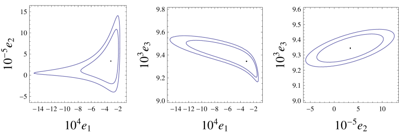
Figure 1: Here, it is shown the result of the bayesian analysis of the model. We use the Constitution (constitution ) data set consisting in 397 SNIa. The best fit value for our parameters $e_{1}=A_{1}(0)/c$, $e_{2}=cA_{2}(0)$ and $e_{3}=t_{0}$ is shown with confidence contours showing the $68.97\%$ and $90\%$ regions.

Using the numerical value for the parameters and the relation (12) we can find an explicit expression for the density parameter as a function of $A_{2}$. Clearly the solution with $\omega_{\perp}=-1/2$ satisfy the requirement for a void solution, as we mention in the last paragraph. The results of the numerical analysis gives a very small value for $A_{2}(0)$, which does not permit us to estimate the value for $\Omega_{M}(z=0)$. The same happens using the Union 2 data set Union2 . The results of the fitting process is shown in Fig.(2). In the first case $\chi^{2}_{red}=1.18$ and in the second one $\chi^{2}_{red}=0.98$, showing that this is a quite good model.

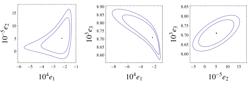
Figure 2: The figure shows the result of the bayesian analysis of the model. We use the Union 2 (Union2 ) data set. The best fit value for our parameters $e_{1}=A_{1}(0)/c$, $e_{2}=cA_{2}(0)$ and $e_{3}=t_{0}$ is shown with confidence contours showing the $68.97\%$ and $90\%$ regions.

IV.2 Case $\omega_{\perp}=-\frac{1}{3}$.

Here $\alpha=2$ and from Eq.(30), we get

$$A_{2}(z)=\frac{1}{\sqrt{c}}\,\sin\left[\frac{\sqrt{c}}{2\,c_{1}}\,\log(1+z)\right]=\frac{1}{\sqrt{c}}\,\sin\left[\frac{\sqrt{c}\,t_{0}}{A_{1}(0)}\,\log(1+z)\right].$$ (32)

Here, the solutions will be a $\sin$ or $\sinh$function, depending on the sign of the $c$ constant. Although it is possible to write down in explicit form the luminosity distance, and then test it under a bayesian analysis, we get that $k(A_{2})\propto A_{2}^{2}$, and thus leading to a FRW metric form and no inhomogeneity is obtained, as can be seeing from Eq.(29). Thus, in this case we recover the homogeneous FRW model.

IV.3 Case $\omega_{\perp}=-\frac{2}{3}$.

Another analytical solution can be obtained by using $\omega_{\perp}=-\frac{2}{3}$. In this case $\alpha=1/2$ and the relation $k(A_{2})\propto\sqrt{A_{2}}$ enable us to have a inhomogeneous universe. This also satisfies the criteria of a “void” solutions, because $\omega_{\perp}<-1/3$. However, the bayesian analysis indicate that this model is not appropriated for describing the observations of the SNIa.

Let us consider now the case where the equations expressed by (22) are equals to a constant $C$ different from zero. The general solution for $A_{2}(r)$ it is found to be

$$k(A_{2})=cA_{2}^{-\frac{1+\omega_{\perp}}{\omega_{\perp}}}+\frac{C\,A_{2}^{2}}{1+3\omega_{\perp}},$$ (33)

where the first term corresponds to the homogeneous solution of Eq.(22), i.e., $C=0$ (see Eq.(27)). By taking into account Eqs.(33) and (12) we notice that this class of solution are not permitted, due to the presence of the second term proportional to $A_{2}^{2}$ in Eq.(33). We see that, as $A_{2}\rightarrow\infty$ the matter density parameter $\Omega_{M}$ goes to $\pm\infty$, depending on the global sign of this term (which depends on $C$ and $\omega_{\perp}$). This behavior makes the model unacceptable.

V Conclusions

In this paper we have studied a certain class of inhomogeneous LTB universes, in which the matter component is an inhomogeneous and anisotropic fluid CLdCCS08 ; CdCMS09 , where the radial and tangential pressures are given by $p_{r}=\omega\rho$ and $p_{\bot}=\omega_{\bot}\rho$, respectively. We have found analytical solutions to the system in order to compute explicitly the luminosity distance that was tested with the SNIa observations. We use both the Constitution constitution and Union 2 Union2 data sets. Our equations enable us to find directly, without any arbitrary ansatz, the profile of the density matter $\Omega_{M}$ as a function of the radial coordinate. In this way, the fitting process with observations can fix the value of the density matter, both at $z=0$ and at $z\rightarrow\infty$. We have found that the only model favored by the observations is of the “void” type solution, where $\Omega_{M}$ is a function that increase with the increment of the radial coordinate, leading to a constant asymptotic value. Although we can not determine the current value for the matter density, because of the very low value for $A_{2}(0)$ in the fitting process (see comments at the end of subsection IV), we think that the method could be of interest in the case of nearly FRW inhomogeneous models.

A necessary next step in testing these kind of models is to consider other observational probes. At present there is no agreement about how to proceed in the use of CMB and Large scale structure as additional probes 26 ; 35 even in the simplest LTB dust model. Although progress has been made cmb_dp , we need to understand better the evolution of density perturbations in LTB spacetimes. Because at present we do not have a clear framework to address these problems, we have to look for additional observational probes. For example, in a recent work dePutter:2012zx the authors used galaxy ages GA . The results still favored the $\lambda$CDM model against the simplest dust LTB solution, in agreement with other probes.

Note also that we have not addressed the stability issue of our models. But, since it becomes similar to a FRW-type of model (see expression (23)) we expect that it model studied here is effectively stable. The demonstration could be carried in a similar way than that followed in the FRW case. However, here the situation become more complicate due to its homogeneity. We expect to address these points in the coming future.

References

- (1) M. Sullivan, Lect. Note Phys. 800 59 (2010).
- (2) A. G. Riess et al, ApJ 116 1009 (1998).
- (3) S. Perlmutter et al, ApJ 517 565 (1999).
- (4) S. del Campo, R. Herrera and D. Pavón,Phys. Rev. D 78 021302 (2008)(RC).
- (5) D. Huterer and M. S. Turner, Phys. Rev. D 60 081301 (1999).
- (6) Sh. Tsujikawa, arXiv:1004.1493 [astro-ph. CO].
- (7) R. R. Cadwell, Space. Sci. Rev., 148 347 (2009) .
- (8) R. R. Caldwell, R. Dave and P. J. Steinhardt, Phys. Rev. Lett. 80 1582 (1998).
- (9) I. Zlatev, L. Wang and P. J. Steinhardt, Phys. Rev. Lett. 82, 896 (1998).
- (10) T. Chiba, T. Okabe and M. Yamaguchi, Phys. Rev. D 62, 023511 (2000).
- (11) C. Armendariz-Picon, V. F. Mukhanov and P. J. Steinhardt, Phys. Rev. Lett. 85 4438 (2000).
- (12) C. Armendariz-Picon, V. F. Mukhanov and P. J. Steinhardt,Phys. Rev. D 63 103510 (2001).
- (13) R. R. Caldwell, Phys. Lett. B 545 23 (2002).
- (14) S. M. Carroll, M. Hoffman and M. Trodden, Phys. Rev. D 68 023509 (2003).
- (15) S. D. H. Hsu, A. Jenkins and M. B. Wise,Phys. Lett. B 597 270 (2004).
- (16) X. Zhang, F. Q. Wu, Phys. Rev. D 76 023502 (2007).
- (17) H. Wei, S. N. Zhang, Phys. Rev. D 76 063003 (2007).
- (18) S. del Campo, J. C. Fabris, R. Herrera and W. Zimdahl, arXiv:1103.3441 [astro-ph.CO].
- (19) R.A. Daly, A Decade of Dark Energy: 1998 - 2008., (2009) [arXiv:astro-ph / 0901.2724].
- (20) M. Sami, Dark energy and possible alternatives., (2009) [arXiv:hep-th / 0901.0756v1].
- (21) For a review, see E. J. Copeland, M. Sami and S. Tsujikawa, Int. J. Mod. Phys. D 15, 1753 (2006).
- (22) N. Straumann, Mod. Phys. Lett. A 21, 1083 (2006).
- (23) M. Cataldo, P. Labraña, S. del Campo, J. Crisostomo and P. Salgado, Phys. Rev. D 78 104006 (2008).
- (24) M. Cataldo, S. del Campo, P. Minning and P. Salgado, Phys. Rev. D 79 024005 (2009).
- (25) M. Cataldo and S. del Campo, Phys. Rev. D 85 104010 (2012).
- (26) R. Giambo, F. Giannoni, G. Magli and P. Piccione, Class. Quantum Grav. 20, 4943 (2003); idem, Gen. Rel. Grav. 36, 1279 (2004).
- (27) P.D. Lasky and A.W.C. Lun, Phys. Rev. D 74, 084013 (2006).
- (28) P. D. Lasky and K. Bolejko, Class. Quant. Grav. 27, 035011 (2010).
- (29) G. Lemâtre, Ann. Soc. Sci. Bruxelles A 53, 51 (1933); reprinted in Gen. Rel. Grav. 29, 641 (1997).
- (30) R. C. Tolman, Proc. Nat. Acad. Sci. 20, 169 (1934); reprinted in Gen. Rel. Grav. 29, 935 (1997).
- (31) H. Bondi, Mon. Not. R. Astron. Soc. 107, 410 (1947).
- (32) M.-N. Celerier, Prog. Theor. Phys. 353, 63 (2000).
- (33) N. Mustapha, C. Hellaby and G. F. R. Ellis, Mon. Not. Roy. Astron. Soc. 292, 817 (1997).
- (34) H. Iguchi, T. Nakamura and K.-i. Nakao, Prog. Theor. Phys. 108, 809 (2002).
- (35) D. Alonso, J. Garcia-Bellido, T. Haugbolle and J. Vicente, Phys. Rev. D 82, 123530 (2010).
- (36) C. M. Yoo, K. i. Nakao and M. Sasaki, JCAP 1007, 012 (2010)
- (37) C. M. Yoo, K. i. Nakao and M. Sasaki, JCAP 1010, 011 (2010).
- (38) S. February, J. Larena, M. Smith, and C. Clarkson, Mon.Not.Roy.Astron.Soc. 405 (2010) 2231, [arXiv:0909.1479].
- (39) V. Marra and A. Notari, Class.Quant.Grav. 28 (2011) 164004, [arXiv:1102.1015].
- (40) C. Clarkson, T. Clifton, and S. February. JCAP,0906,25 (2009); J. P. Zibin, Phys. Rev. D 78, 043504 (2008); S. February, C. Clarkson and R. Maartens, arXiv:1206.1602 [astro-ph.CO].
- (41) R. de Putter, L. Verde and R. Jimenez, arXiv:1208.4534 [astro-ph.CO].
- (42) R. Jimenez and A. Loeb, Astrophys. J. 573, 37 (2002) [astro-ph/0106145]; H. Wang and T. -J. Zhang, Astrophys. J. 748, 111 (2012) [arXiv:1111.2400 [astro-ph.CO]].
- (43) K. Enqvist and T. Mattsson, JCAP 0702, 019 (2007).
- (44) K. Enqvist, Gen. Rel. Grav. 40, 451 (2008).
- (45) J. Garcia-Bellido and T. Haugbolle, JCAP 0804, 003 (2008).
- (46) G.F.R. Ellis, in proc. School Enrico Fermi, “General relativity and Cosmology”, Ed. R.K. Sachs, Academic Press (NY, 1971).
- (47) M. Hicken et al., Astrophys. J. 700, 1097 (2009).
- (48) R. Amanullah et al., Astrophys. J. 716, 712 (2010).