Early-stage young stellar objects in the Small Magellanic Cloud

Abstract

We present new observations of 34 Young Stellar Object (YSO) candidates in the Small Magellanic Cloud (SMC). The photometric selection required sources to be bright at 24 and 70 $\mu$m (to exclude evolved stars and galaxies). The anchor of the analysis is a set of Spitzer-IRS spectra, supplemented by groundbased 3$-$5 $\mu$m spectra, Spitzer IRAC and MIPS photometry, near-IR imaging and photometry, optical spectroscopy and radio data. The sources’ spectral energy distributions (SEDs) and spectral indices are consistent with embedded YSOs; prominent silicate absorption is observed in the spectra of at least ten sources, silicate emission is observed towards four sources. Polycyclic Aromatic Hydrocarbon (PAH) emission is detected towards all but two sources. Based on band ratios (in particular the strength of the 11.3-$\mu$m and the weakness of the 8.6-$\mu$m bands) PAH emission towards SMC YSOs is dominated by predominantly small neutral grains. Ice absorption is observed towards fourteen sources in the SMC. The comparison of H₂O and CO₂ ice column densities for SMC, Large Magellanic Cloud (LMC) and Galactic samples suggests that there is a significant H₂O column density threshold for the detection of CO₂ ice. This supports the scenario proposed by Oliveira et al. (2011), where the reduced shielding in metal-poor environments depletes the H₂O column density in the outer regions of the YSO envelopes. No CO ice is detected towards the SMC sources. Emission due to pure-rotational $0-0$ transitions of molecular hydrogen is detected towards the majority of SMC sources, allowing us to estimate rotational temperatures and H₂ column densities. All but one source are spectroscopically confirmed as SMC YSOs. Based on the presence of ice absorption, silicate emission or absorption, and PAH emission, the sources are classified and placed in an evolutionary sequence. Of the 33 YSOs identified in the SMC, 30 sources populate different stages of massive stellar evolution. The presence of ice- and/or silicate-absorption features indicates sources in the early embedded stages; as a source evolves, a compact H ii region starts to emerge, and at the later stages the source’s IR spectrum is completely dominated by PAH and fine-structure emission. The remaining three sources are classified as intermediate-mass YSOs with a thick dusty disc and a tenuous envelope still present. We propose one of the SMC sources is a D-type symbiotic system, based on the presence of Raman, H and He emission lines in the optical spectrum, and silicate emission in the IRS-spectrum. This would be the first dust-rich symbiotic system identified in the SMC.

1 Introduction

Star formation is a complex interplay of various chemo-physical processes. During the onset of gravitational collapse of a dense cloud, dense cores can only develop if heat can be dissipated. The most efficient cooling mechanisms are via radiation through fine-structure lines of carbon and oxygen, and rotational transitions in abundant molecules such as water (e.g., van Dishoeck, 2004). These cooling agents all contain at least one metallic atom. Furthermore, dust grains are crucial in driving molecular cloud chemistry, as dust opacity shields cores from radiation, and grain surfaces enable chemical reactions to occur that would not happen in the gas phase. These facts suggest that metallicity is an important parameter to explore in understanding star formation. However, most of what is known about the physics of star formation is deduced from observations in solar-metallicity Galactic star forming regions. The nearest templates for the detailed study of star formation under metal-poor conditions are the Magellanic Clouds (MCs), with ISM metallicities of $Z_{\rm SMC}\sim 0.2\,Z_{\odot}$ and $Z_{\rm LMC}\sim 0.4\,Z_{\odot}$, respectively for the SMC and LMC (e.g., Russell & Dopita, 1992). Even over the metallicity range covered by the Galaxy and the MCs, cooling and chemistry rates, and star formation timescales could be affected (Banerji et al., 2009). The low metallicity of the SMC in particular is typical of galaxies during the early phases of their assembly, and studies of star formation in the SMC provide a stepping stone to understanding star formation at high redshift where these processes cannot be directly observed.

The Spitzer Space Telescope (Spitzer, Werner et al., 2004) finally allowed the identification of sizable samples of Young Stellar Objects (YSOs) in the MCs. The Spitzer Legacy Programs (SAGE, Meixner et al. 2006; SAGE-SMC, Gordon et al. 2011a) have identified 1000s of previously unknown YSOs, both in the LMC and the SMC (Whitney et al. 2008; Gruendl & Chu 2009; Sewiło et al in preparation). Follow-up spectroscopic programmes have provided unique insight into the abundances of ices in Magellanic YSOs, revealing differences in the composition of circumstellar material at lower metallicity (Oliveira et al., 2009, 2011; Shimonishi et al., 2010; Seale et al., 2011).

In this paper we present a sample of 34 photometrically selected YSO candidates in the SMC, observed with Spitzer’s InfraRed Spectrograph (IRS, Houck et al., 2004). Based on the properties of their IRS spectra and a variety of multi-wavelength diagnostics, we classify 33 sources as YSOs in the SMC (27 previously unknown) and 1 source as a symbiotic system. This paper is organised as follows. After describing the sample selection and the different observations, the spectral properties of the SMC sources are analysed in detail in Section 4, with the aim of assessing the sources’ evolutionary stage. We describe the SED properties and modelling, dust and ice absorption, polycyclic aromatic hydrocarbon (PAH), ionic fine structure and H₂ emission, and the properties of optical counterparts to the infrared (IR) sources. The source classification and their evolutionary status is then discussed in Section 5. Section 6 describes the process that allowed us to identify one of the sources as the first D-type symbiotic system in the SMC.

2 Defining the YSO sample

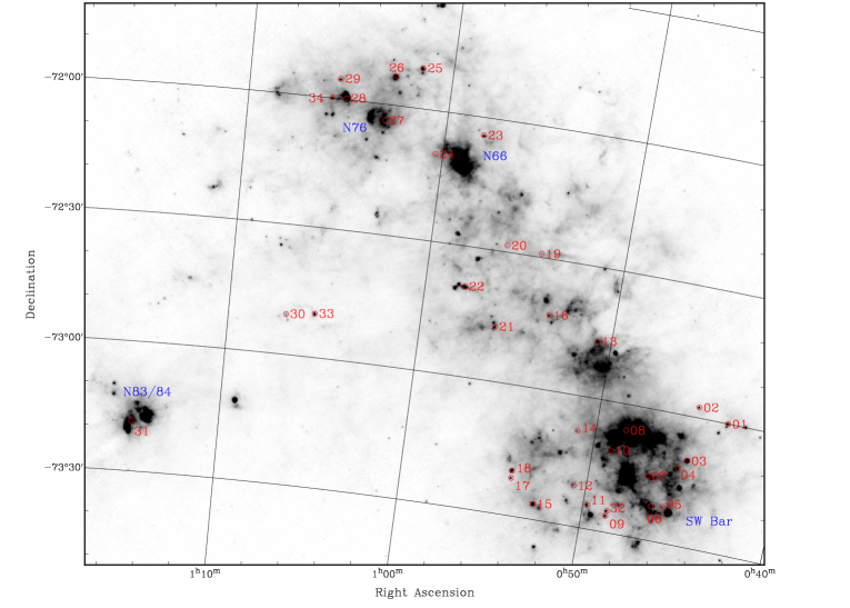
Figure 1: SAGE-SMC MIPS 70-$\mu$m image showing the location of the 34 YSO candidates (red circles and labels); sources #01 to 31 were first identified in this survey (see also Oliveira et al., 2011; van Loon et al., 2010b), while sources #32 (MSX SMC 79), #33 (IRAS 01039$-$7305) and #34 (IRAS 01042$-$7215) were identified by van Loon et al. (2008). The star forming regions discussed in Section 4.3 are labelled in blue.

The S³MC survey (Bolatto et al., 2007) imaged the main body of the SMC (central 3 square degrees) in all seven Spitzer photometric bands, using the Infrared Array Camera (IRAC, Fazio et al., 2004) and the Multiband Imaging Photometer for Spitzer (MIPS, Rieke et al., 2004). The resulting photometric catalogue was used to select the present YSO sample as described below.

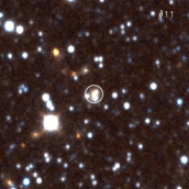
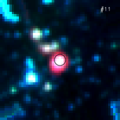
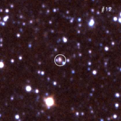
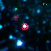
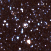
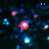
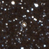
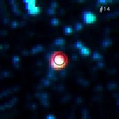
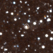
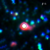
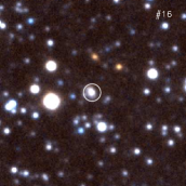
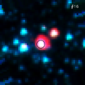
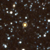
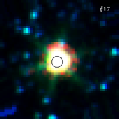
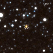
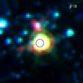
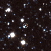
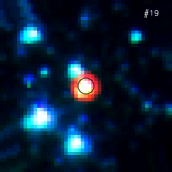
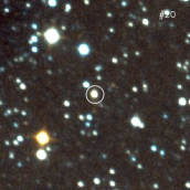
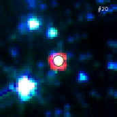
Figure 1: Continued.

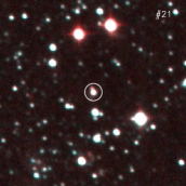
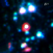
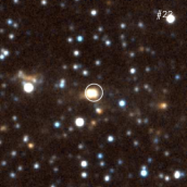
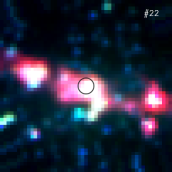
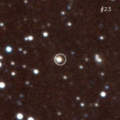
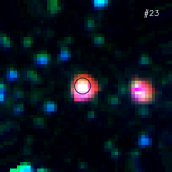
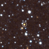
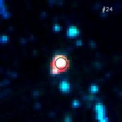
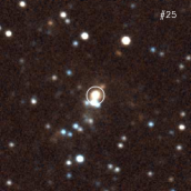
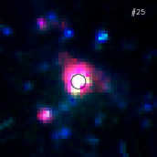
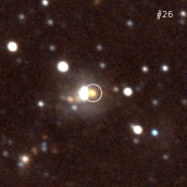
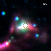
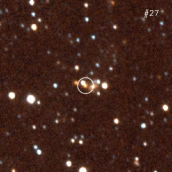
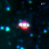
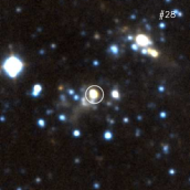
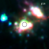
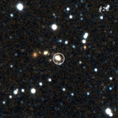
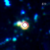
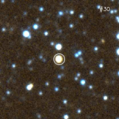
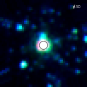
Figure 2: continued

The near- and mid-IR colours of evolved stars can be as red as embedded YSOs (especially carbon stars, which are common in the SMC). This makes the 70 $\mu$m photometry critical in identifying YSOs with cold dust (as opposed to the warm dust surrounding evolved stars). Thus, we selected targets with detections in all IRAC bands and at 24 and 70 $\mu$m. We also imposed a 10 mJy lower limit to the 8 and 24 $\mu$m fluxes so that the sources are suitable for Spitzer spectroscopy. From the 160 objects with 70 $\mu$m detections, we were left with 46 candidates. By cross-correlating their positions with the SIMBAD database and the Spitzer’s Reserved Object Catalogue, we rejected 15 objects which might be (or are near to) evolved stars or planetary nebulae. The 31 remaining targets have colours $[3.6]-[5.8]>1.35$ mag and $[8]-[24]>2.75$ mag, typical for embedded YSOs (Rho et al., 2006). Background galaxies can also have colours similar to those of YSOs (Eisenhardt, Stern & Brodwin, 2004). However, the selected YSO candidates are bright, sit well above the bulk of background galaxy contamination (Lee et al., 2006; Jørgensen et al., 2006), and most are located in active regions of star formation (Fig.1). Thus they are likely genuine YSOs and not more uniformly distributed evolved stars or background galaxies. YSO candidates separate better from the bulk SMC population in colour–magnitude diagrams, rather than colour–colour diagrams (Whitney et al. 2008; Sewiło et al. in preparation), as demonstrated in Fig. 2. Our selection criteria imply the final sample is composed of massive YSOs ($M\ga 10M_{\odot}$). The sample is obviously not complete but it is ideally designed to identify massive YSOs that can be the subjects of a detailed spectroscopic analysis.

Our strategy has proved very successful, with all but one of the 31 candidates confirmed as an embedded YSO or compact H ii region (Section 4). We add to the SMC sample the three YSOs identified by van Loon et al. (2008), MSX SMC 79, IRAS 01039$-$7305 and IRAS 01042$-$7215, based on the appearance of their 3$-$4 $\mu$m spectra(Section 3.3). The locations of these 34 YSO candidates superposed on a 70-$\mu$m MIPS image of the SMC are shown in Fig. 1. Fig. 2 shows $[3.6]-[8.0]\,vs.\,[8.0]-[24]$ colour–colour and $[8.0]\,vs\,[8.0]-[24]$ colour–magnitude diagrams for the 34 YSO candidates, together with the field SMC population (Gordon et al., 2011a).

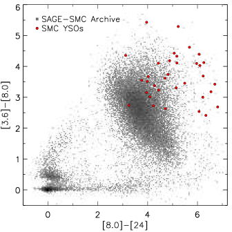
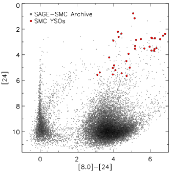
Figure 2: Colour–colour and colour–magnitude diagrams for the YSO candidates (filled red circles), as well as the field SMC population (grey scale).

3 Observations and catalogues

3.1 Spitzer-IRS and MIPS-SED spectroscopy

The mid-IR, low-resolution spectra of the 31 candidate YSOs were obtained using the Spitzer-IRS and the spectral energy distribution (SED) mode of MIPS (Rieke et al., 2004) on board Spitzer, taken as part of the SMC-Spec program (PID: 50240, P.I.: G.C. Sloan). This GTO programme aimed at providing a comprehensive spectroscopic survey of the SMC. Scientifically its goals were to study dust in nearly every stage of its life cycle in the SMC in order to assess how the interactions of dust and its host galaxy differ from more metal-rich systems like the Galaxy and the LMC. The programme was designed to provide the SMC counterpart of the LMC SAGE-Spec programme (Kemper et al., 2010), albeit at a smaller scale. The SMC observations targeted important classes generally underrepresented in the Spitzer archive of SMC sources, such as YSOs and compact H ii regions, objects in transition to and from the asymptotic giant branch, and supergiants. The aforementioned three additional objects from van Loon et al. (2008) were initially thought to be evolved stars; their Spitzer-IRS spectra were obtained as part of a cycle 1 GTO programme (PID: 3277, P.I.: M. Egan).

The IRS observations of the point sources in SMC-Spec were performed in staring mode, using the Short-Low and Long-Low modules (SL and LL, respectively). The 8- and 24-$\mu$m fluxes were used to set exposure times, aiming at signal-to-noise ratios of $\sim 60$ in SL and $\sim 30$ in LL. The archival spectra mentioned previously were also obtained in the SL and LL staring modes. All spectra were reduced following standard reduction techniques. Flat-fielded images from the standard Spitzer reduction pipeline (version S18.18) were background subtracted and cleaned of “rogue” pixels and artefacts. Spectra were extracted individually for each data collection event (DCE) and co-added to produce one spectrum per nod position. Individual spectra are extracted both using optimal and tapered extraction; optimal extraction uses super-sampled point-spread function (PSF) profiles to weight the pixels from the spatial profiles, while tapered column extraction integrates the flux in a spectral window that expands with wavelength (Lebouteiller et al., 2010). For each extraction, the nods were then combined to produce a single spectrum per order, rejecting “spikes” that appear in only one of the nod positions. Finally, the spectra of all the segments were combined including the two bonus orders that are useful in correcting for discontinuities between the orders.

While for point sources optimal extraction produces the best signal-to-noise ratio, tapered extraction performs better if the source is extended (Lebouteiller et al., 2010). Some of the sources in our sample could be marginally extended; we opt to use optimal extracted spectra but check the veracity and strength of the spectral features against the tapered extraction spectra. The strength of relevant emission features (Sections 4.3 and 4.4) is measured by first fitting a series of line segments to the continua on either side of feature and then integrating in $F_{\lambda}$ space.

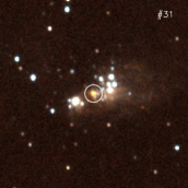
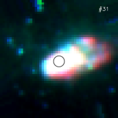
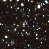
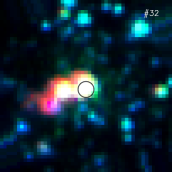
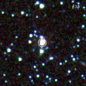
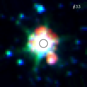
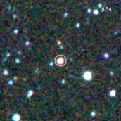
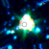
Figure 3: continued

For 10 objects in the sample (see Table 4) we also have MIPS-SED spectra, covering the wavelength range 52$-$90 $\mu$m, as described in van Loon et al. (2010b). The IRS and MIPS-SED Spitzer spectra are shown in Fig. 3 (selected examples) and Appendix B (complete sample).

3.2 SAGE-SMC photometric data

The SAGE-SMC (Surveying the Agents of Galaxy Evolution in the Tidally-Stripped, Low Metallicity Small Magellanic Cloud) Spitzer Legacy programme (PID: 40245, P.I.: K. Gordon) mapped almost the entire SMC using IRAC and MIPS. Gordon et al. (2011a) provide a full discussion of the observations, data reduction and catalogue generation; we highlight here only the more relevant details.

In the overlap region, the SAGE-SMC and (reprocessed) S³MC images were combined to produce mosaic images from which photometric catalogues were created (we use the “Single Frame + Mosaic Photometry” catalogue). There is a systematic offset between the IRAC photometry in the SAGE-SMC and S³MC catalogues (Gordon et al., 2011a); since there is an excellent agreement between the SAGE-SMC fluxes and those predicted from the IRAC calibration stars we adopt the IRAC SAGE-SMC catalogue fluxes. Due to updated processing and improved calibrations, the S³MC and SAGE-SMC MIPS fluxes are also different (see Gordon et al., 2011a, for full details); we also adopt the MIPS SAGE-SMC catalogue fluxes. Catalogue fluxes are listed in Table LABEL:table1.

Due to the complexity of the multiple datasets, the SAGE-SMC catalogue relies on a stringent set of rules to create the final catalogues, designed to maximise reliability rather than completeness (Gordon et al., 2011b). Therefore, the SAGE-SMC catalogues do not provide fluxes for all the IR sources in our target list: even though the images clearly show a point source, a few sources are missing the shortest or all IRAC band fluxes for a variety of reasons. Some YSOs sit in regions where there is a complex structure of extended emission (characteristic of star forming environments), and may be also marginally extended. Other issues can arise during the source extraction and band merging processes causing a particular source not to make it into the final IRAC photometric catalogue, for instance variability and source confusion. As part of their paper on SMC YSOs identified using SAGE-SMC images and catalogues, Sewiło et al. (in preparation) visually inspected all the images of the 34 YSO candidates in this sample, and performed aperture photometry on the mosaic images. When SAGE-SMC catalogue fluxes are unavailable, Table LABEL:table1 lists extracted aperture fluxes (identified by $*$). The adopted aperture sizes are $5\arcsec$ for the IRAC bands, and $8\arcsec$ and $15\arcsec$ respectively for MIPS 24 and 70 $\mu$m.

3.3 Thermal-infrared ground-based spectroscopy

L-band (2.8$-$4.1 $\mu$m) spectra of eleven bright sources in the SMC sample (Table 4) were obtained with the Infrared Spectrometer And Array Camera (ISAAC) at the European Southern Observatory (ESO) Very Large Telescope (VLT) at Paranal, on the nights of 2006 October 28 and 29 (ESO Programme 078.C-0338, P.I.: J.M. Oliveira) to search for H₂O ice absorption at 3 $\mu$m. The standard IR technique of chopping and nodding was employed to cancel the high background. The resolving power was $\lambda/\Delta\lambda\approx 500$. Exposure times varied between 60 and 105 min. The hydrogen lines in the standard stars left remnants of at most a few per cent of the continuum level. Telluric lines were used to calibrate the wavelength scale to an accuracy of $\Delta\lambda\approx 0.002$ $\mu$m.

M-band spectra of five bright SMC objects (Table 4) were also obtained with ISAAC at the VLT, on the nights of 2009 November 4 and 5 (ESO Programme 084.C-0955, P.I.: J.M. Oliveira) to search for the CO ice feature at 4.67 $\mu$m. Exposure times varied between 45 and 90 min. The M-band spectra were obtained and reduced in the same way as the L-band spectra. Telluric lines were used to calibrate the wavelength scale to an accuracy of $\Delta\lambda\approx 0.003$ $\mu$m.

Acquisition for the L-band spectroscopy was done using high spatial resolution L^′-band images ($\lambda=3.8$ $\mu$m). Magnitudes were obtained using aperture photometry on the targets and spectral standard stars observed at regular intervals during each night. Magnitudes were converted to fluxes using the following conversion: a 16-mag star has a flux of $9.414\times 10^{-5}$ Jy. These resulting fluxes (Table LABEL:table1) were used to flux-calibrate the L-band spectra.

Some of these spectra have been published previously; van Loon et al. (2008) first identified MSX SMC 79 (source #32), IRAS 01039$-$7305 (#33) and IRAS 01042$-$7215 (#34) as YSOs based on their L-band spectra; Oliveira et al. (2011) discussed the ice features of sources #03, 17, 18 and 34; they did not discuss the spectra of source #33 since the ice detections are uncertain.

3.4 Near- and mid-infrared ground-based imaging

The near-infrared imaging observations were performed with the SOFI (Son OF ISAAC) imager at the New Technology Telescope (NTT) at ESO La Silla, between 2006 October 1 and 2006 November 10 in service mode (ESO Programme 078.C-0319, P.I.: J.Th. van Loon). Images were obtained with the $J_{s}$ and $K_{s}$ filters using the $0\hbox to0.0pt{.\hss}^{\prime\prime}288$ pixel^-1 plate scale, with a total integration time of 11 min per filter. The total integration time was split into jittered 1 min exposures to allow for efficient sky removal. For each filter, the jittered images were reduced and combined using standard infrared reduction steps implemented within ESO’s data reduction pipelines: detector cross-talk correction, flatfield correction, sky subtraction and shift-addition of jittered frames. Photometric calibration was done using dedicated standard star observations; these were observed several times per night in order to estimate magnitude zeropoints. Since zeropoints were well behaved, we adopted a single value to calibrate all observations: $z_{J_{s}}=23.09\pm 0.02$ mag and $z_{K_{s}}=22.37\pm 0.04$ mag. PSF photometry was performed using the daophot package (Stetson, 1987) within iraf. Typical full-width at half-maximum (FWHM) of the stellar profiles were 3.8 and 3.6 pixels, corresponding to respectively $1\hbox to0.0pt{.\hss}^{\prime\prime}1$ and $1\hbox to0.0pt{.\hss}^{\prime\prime}0$ in the $J_{s}$- and $K_{s}$-bands. Aperture correction was performed using bright PSF stars. Magnitudes were converted to fluxes using the following conversion: a 16-mag star has fluxes of $6.112\times 10^{-4}$ Jy and $2.584\times 10^{-4}$ Jy, respectively in $J_{s}$ and $K_{s}$. Fluxes are listed in Table LABEL:table1. In Appendix C, $J_{s}K_{s}$ colour composite images are shown for each target (Fig. 16), together with Spitzer/IRAC [3.6]-[5.8]-[8] colour composites. Some sources sit in complex cluster-like environments; we carefully investigated each image to identify the redder source as the counterpart for the mid-IR sources (these identifications were usually very obvious).

SOFI imaging was obtained only for the original 31 objects, not for the additional objects identified by van Loon et al. (2008). However, source #32 is in the SOFI field-of-view of source #09 and $J_{s}$ and $K_{s}$ fluxes were also measured. For the remaining two sources (#33 and 34) we use $JHK_{s}$ fluxes and images from the IR Survey Facility (IRSF, Kato et al., 2007).

The 21 brightest mid-IR objects were imaged with the VLT Imager and Spectrograph for the IR (VISIR) at ESO, Paranal, in service mode over the period 2006 September 4 to October 3 (ESO Programme 078.C-0319, P.I.: J.Th. van Loon). Images were obtained through the narrow-band PAH2 filter (centered at $\lambda=11.25$ $\mu$m, half-band width $\Delta\lambda=0.59$ $\mu$m). Eight standard stars with flux densities in the range 5$-$11 Jy were observed for photometric calibration. The plate scale was $0\hbox to0.0pt{.\hss}^{\prime\prime}075$, providing a field-of-view of $19\arcsec\times 19\arcsec$. The standard IR technique of chopping and nodding was employed to cancel the high background. Integration times were 24 minutes, split in 16 exposures of 23 chop cycles each. The individual exposures were combined and corrected for instrumental effects using version 1.5.0 of the VISIR pipeline. Photometry was performed by collecting the counts within a circular aperture centered on the zero-order maximum of the diffraction pattern, avoiding the first Airy ring; if the source was not detected upper limits were calculated. Table LABEL:table1 lists the fluxes.

3.5 Ancillary multi-wavelength data

3.5.1 Optical spectroscopy

Our optical spectroscopy was obtained using the Double-Beam Spectrograph (DBS) mounted on the Nasmyth focus of the Australian National University 2.3-m telescope at Siding Spring Observatory. More information on the instrument can be found in Rodgers, Conroy & Bloxham (1988). Standard iraf routines were used for the data reduction (bias subtraction, flat fielding, wavelength calibration). The blue and red spectra were joined in the interval 6160$-$6300 Å; the joined spectra cover the wavelength range 3600$-$9500 Å. Spectral standard stars, observed with the same instrumental setup as the programme objects, were used to provide a relative flux calibration for each object. Telluric features were removed by observing white dwarf standards with few intrinsic spectral features. The final spectra have an effective resolution of $\sim 4.5$ Å.

Optical spectra were obtained for 32 objects (Appendix D, Fig. 4). At the position of the IR source, source #24 shows no point source at optical wavelengths, only extended emission. There is clearly a point source in the $J_{s}$-band (Fig. 16) but it is the faintest object in the sample (Table LABEL:table1); thus it was too faint to obtain an optical spectrum. The position of IR source #31 sits between two bright optical sources; in Fig. 16 it is clear that this region is very complex with many bright sources at short wavelengths as well as bright IR sources. Thus no optical spectrum was obtained for this source.

For sources #05, 06 and 29 the optical spectra exhibit only Balmer absorption lines, i.e. the spectra are typical of more evolved stars. Since these objects are also very faint in the $J_{s}$-band (Table LABEL:table1) it is unlikely the obtained optical spectra are associated with the IR source. For sources #02, 10, 11, 14, 16, 17, 18, 23 and 34 the spectra only show H$\alpha$ emission thus we perform no further analysis of their optical spectra. For the remaining 20 sources we analyse the optical spectra in detail (Section 4.5).

3.5.2 Radio data

Radio free-free emission from (ultra-)compact H ii regions is a common signpost of massive star formation. Using all available archival data from the Australia Telescope Compact Array (ATCA) and the Parkes radio telescope, Wong et al. (2011a) and Crawford et al. (2011) created new high-sensitivity, high-resolution radio-continuum images of the SMC at 1.42, 2.37, 4.80 and 8.64 GHz (wavelengths respectively 20, 13, 6 and 3 cm), as well as point source catalogues (Wong et al., 2011b, 2012). Of the 34 objects in the sample, 11 sources have radio-continuum detections at at least 2 frequencies. Of these, 8 are radio point sources found within $4\arcsec$ of the IR source (the positional accuracy at 20 and 13 cm). Sources #08 and 31 are in complex and extended H ii regions and therefore the source position is less certain; there is no point source at the position of source #15 but we clearly see an extended radio-continuum object. Radio spectral indices ($S_{\nu}\propto\nu^{\alpha}$) for these sources are $\alpha\ \vbox{\hbox{$>$}\offinterlineskip\hbox{$\sim$}}-0.3$, consistent with their classification as compact H ii regions (e.g., Filipović et al., 1998) — background galaxies are dominated by synchrotron emission with a steeper spectral index. The sources detected at radio wavelengths are the most luminous in our sample (Section 4.1).

Table 1: Infrared fluxes (in mJy) for the SMC YSO candidates. Spitzer photometry is from the SAGE-SMC catalogue (Gordon et al., 2011a); when catalogue photometry is unavailable, aperture photometry fluxes are used (indicated by $*$). Listed $J_{s}K_{s}$ fluxes are from this work, except for fluxes of sources #32 and 33 that are from the IRSF catalogue (Kato et al., 2007). Source IDs are from the S³MC catalogue, unless stated otherwise. S³MC objects were identified by Bolatto et al. (2007). Some sources were identified spectroscopically using IRS and MIPS-SED spectra by van Loon et al. (2008, 1), van Loon et al. (2010b, 2) and Oliveira et al. (2011, 3); Martayan et al. (2007, 4) identified source #20 as a candidate Herbig B[e] star. Source classification is discussed in Sections 5 and 6.

#	RA & Dec (J2000)	$J_{s}$	$K_{s}$	$L^{\prime}$	$F_{3.6}$	$F_{4.5}$	$F_{5.8}$	$F_{8}$	$F_{11.3}$	$F_{24}$	$F_{70}$	source ID	Ref.
01	00 43 12.86 $-$72 59 58.3	0.339 $\pm$ 0.029	0.341 $\pm$ 0.030		*2.56 $\pm$ 0.30	*1.98 $\pm$ 0.27	*10.35 $\pm$ 0.62	*25.74 $\pm$  0.98	$<$ 6	337.6 $\pm$  1.7	3316 $\pm$ 21	004312.85$-$725958.30
												IRAS 00413$-$7316
02	00 44 51.87 $-$72 57 34.2	0.258 $\pm$ 0.016	0.937 $\pm$ 0.047	7.76 $\pm$ 0.75	5.76 $\pm$ 0.17	9.92 $\pm$ 0.23	15.73 $\pm$ 0.36	31.69 $\pm$  0.45	33 $\pm$  4	555.4 $\pm$  4.9	1620 $\pm$ 18	IRAS 00429$-$7313	2
03	00 44 56.30 $-$73 10 11.8	0.210 $\pm$ 0.030	3.583 $\pm$ 0.171	82.75 $\pm$ 7.98	40.27 $\pm$ 0.66	*82.85 $\pm$ 1.00	150.60 $\pm$ 1.60	193.10 $\pm$  2.46	164 $\pm$ 10	2470.0 $\pm$ 12.4	12440 $\pm$ 60	IRAS 00430$-$7326	2, 3
04	00 45 21.26 $-$73 12 18.7	0.977 $\pm$ 0.028	1.010 $\pm$ 0.051		1.78 $\pm$ 0.18	2.17 $\pm$ 0.06	2.92 $\pm$ 0.19	4.59 $\pm$  0.63		39.3 $\pm$  0.4	917 $\pm$ 11	004521.26$-$731218.68
05	00 45 47.51 $-$73 21 42.4	0.081 $\pm$ 0.004	0.527 $\pm$ 0.024		3.33 $\pm$ 0.08	5.81 $\pm$ 0.07	8.18 $\pm$ 0.14	12.20 $\pm$  0.24		59.4 $\pm$  0.5	281 $\pm$  6
06	00 46 24.45 $-$73 22 07.1	0.077 $\pm$ 0.006	0.363 $\pm$ 0.024	3.89 $\pm$ 0.38	2.85 $\pm$ 0.14	8.82 $\pm$ 0.17	14.40 $\pm$ 0.31	20.40 $\pm$  0.48	$<$ 6	192.5 $\pm$  0.9	2154 $\pm$ 20	004624.46$-$732207.30	2
07	00 46 51.72 $-$73 15 25.3	0.078 $\pm$ 0.008	0.101 $\pm$ 0.012		*1.71 $\pm$ 0.25	*1.08 $\pm$ 0.20	*9.04 $\pm$ 0.58	*21.60 $\pm$  1.00		42.5 $\pm$  0.4	776 $\pm$ 11	004651.71$-$731525.34
08	00 48 25.83 $-$73 05 57.3	0.166 $\pm$ 0.014	0.316 $\pm$ 0.023		2.07 $\pm$ 0.08	3.25 $\pm$ 0.06	8.76 $\pm$ 0.16	19.30 $\pm$  0.44	19 $\pm$  2	592.8 $\pm$  5.2	7779 $\pm$ 55	004825.83$-$730557.29
09	00 48 41.78 $-$73 26 15.3	0.141 $\pm$ 0.015	0.146 $\pm$ 0.028		*1.93 $\pm$ 0.26	0.98 $\pm$ 0.04	3.01 $\pm$ 0.10	7.00 $\pm$  0.43	$<$ 6	239.4 $\pm$  1.0	1875 $\pm$ 18	004841.77$-$732615.25
10	00 49 01.64 $-$73 11 09.6	0.086 $\pm$ 0.008	0.163 $\pm$ 0.016		*2.49 $\pm$ 0.30	0.80 $\pm$ 0.13	5.06 $\pm$ 0.27	13.30 $\pm$  0.95	$<$ 6	708.7 $\pm$  4.0	3109 $\pm$ 25	004901.63$-$731109.60
11	00 49 44.57 $-$73 24 32.8	0.121 $\pm$ 0.009	0.166 $\pm$ 0.015		*1.59 $\pm$ 0.24	0.52 $\pm$ 0.03	3.39 $\pm$ 0.17	7.13 $\pm$  0.46		47.5 $\pm$  0.5	*900 $\pm$ 73	004944.57$-$732432.75
12	00 50 40.25 $-$73 20 37.0	0.090 $\pm$ 0.007	0.124 $\pm$ 0.011		0.66 $\pm$ 0.03	0.46 $\pm$ 0.01	3.02 $\pm$ 0.07	7.11 $\pm$  0.19		71.3 $\pm$  0.5	452 $\pm$  6	005040.24$-$732036.99
13	00 50 43.24 $-$72 46 56.2	0.252 $\pm$ 0.021	0.336 $\pm$ 0.024		1.63 $\pm$ 0.27	1.27 $\pm$ 0.05	5.89 $\pm$ 0.18	16.60 $\pm$  0.54	8 $\pm$  1	589.2 $\pm$  3.6	2762 $\pm$ 28	005043.23$-$724656.24
14	00 50 58.09 $-$73 07 56.8	0.391 $\pm$ 0.019	0.817 $\pm$ 0.048		2.11 $\pm$ 0.04	2.42 $\pm$ 0.03	4.95 $\pm$ 0.07	13.50 $\pm$  0.19		114.3 $\pm$  1.1	461 $\pm$  6	005058.09$-$730756.78
15	00 52 38.84 $-$73 26 23.9	0.227 $\pm$ 0.013	0.246 $\pm$ 0.020		1.57 $\pm$ 0.20	1.04 $\pm$ 0.06	6.98 $\pm$ 0.22	20.50 $\pm$  0.51	14 $\pm$  6	610.7 $\pm$  3.4	2695 $\pm$ 19	005238.84$-$732623.92
												IRAS 00509$-$7342
16	00 53 25.36 $-$72 42 53.2	0.364 $\pm$ 0.022	0.369 $\pm$ 0.025		0.84 $\pm$ 0.10	0.67 $\pm$ 0.02	4.03 $\pm$ 0.19	13.50 $\pm$  0.57	19 $\pm$  4	282.0 $\pm$  1.5	1226 $\pm$ 14	005325.36$-$724253.20
												IRAS 00516$-$7259
17	00 54 02.31 $-$73 21 18.6	0.357 $\pm$ 0.022	2.244 $\pm$ 0.120	26.41 $\pm$ 2.55	19.50 $\pm$ 0.25	46.30 $\pm$ 0.66	78.40 $\pm$ 0.71	113.00 $\pm$  0.91	69 $\pm$ 10	496.5 $\pm$  3.5	1669 $\pm$ 14	005402.30$-$732118.70	2, 3
18	00 54 03.36 $-$73 19 38.4	0.247 $\pm$ 0.022	1.104 $\pm$ 0.060	18.61 $\pm$ 1.80	12.50 $\pm$ 0.18	38.60 $\pm$ 0.37	84.20 $\pm$ 0.78	125.00 $\pm$  1.02	91 $\pm$  7	824.6 $\pm$  5.6	3987 $\pm$ 25	005403.36$-$731938.30	2, 3
19	00 54 19.16 $-$72 29 09.6	0.249 $\pm$ 0.009	0.287 $\pm$ 0.012		1.27 $\pm$ 0.03	3.72 $\pm$ 0.05	10.80 $\pm$ 0.15	37.90 $\pm$  0.34	76 $\pm$  3	522.6 $\pm$  3.1	319 $\pm$  5	005419.16$-$722909.63
20	00 56 06.38 $-$72 28 28.1	0.731 $\pm$ 0.048	0.877 $\pm$ 0.045		2.74 $\pm$ 0.06	4.28 $\pm$ 0.07	6.81 $\pm$ 0.11	18.40 $\pm$  0.20		83.8 $\pm$  0.7	221 $\pm$  3	005606.37$-$722828.05	4
21	00 56 06.50 $-$72 47 22.7	0.075 $\pm$ 0.013	0.167 $\pm$ 0.021		1.14 $\pm$ 0.05	1.15 $\pm$ 0.02	3.75 $\pm$ 0.11	7.77 $\pm$  0.27	$<$ 6	269.3 $\pm$  1.8	1081 $\pm$ 13	005606.49$-$724722.66
22	00 57 57.11 $-$72 39 15.4	0.330 $\pm$ 0.021	0.655 $\pm$ 0.048	2.77 $\pm$ 0.27	3.46 $\pm$ 0.63	3.80 $\pm$ 0.12	6.04 $\pm$ 0.23	8.19 $\pm$  0.66	$<$ 6	243.8 $\pm$  1.6	3276 $\pm$ 29	005757.10$-$723915.40
												IRAS 00562$-$7255
23	00 58 06.41 $-$72 04 07.3	0.347 $\pm$ 0.015	0.385 $\pm$ 0.020		1.19 $\pm$ 0.14	0.86 $\pm$ 0.03	4.89 $\pm$ 0.17	11.80 $\pm$  0.67	$<$ 6	321.1 $\pm$  2.5	1442 $\pm$ 17	005806.41$-$720407.32
												IRAS 00563$-$7220
24	01 00 22.32 $-$72 09 58.1	0.072 $\pm$ 0.003	0.469 $\pm$ 0.023		2.45 $\pm$ 0.05	4.04 $\pm$ 0.06	5.90 $\pm$ 0.08	10.20 $\pm$  0.13		43.6 $\pm$  0.5	202 $\pm$  4
25	01 01 31.70 $-$71 50 40.3	0.348 $\pm$ 0.027	0.386 $\pm$ 0.047		*2.79 $\pm$ 0.32	0.91 $\pm$ 0.17	4.55 $\pm$ 0.26	11.90 $\pm$  1.39	$<$ 6	550.7 $\pm$  2.3	3875 $\pm$ 19	010131.69$-$715040.30
26	01 02 48.54 $-$71 53 18.0	0.167 $\pm$ 0.011	0.482 $\pm$ 0.028		*3.57 $\pm$ 0.36	*4.58 $\pm$ 0.41	5.07 $\pm$ 0.24	7.52 $\pm$  0.64	$<$ 6	288.2 $\pm$  2.1	5616 $\pm$ 30	010248.54$-$715317.98
27	01 03 06.14 $-$72 03 44.0	0.073 $\pm$ 0.005	0.154 $\pm$ 0.009		0.48 $\pm$ 0.09	0.37 $\pm$ 0.01	2.01 $\pm$ 0.12	*16.26 $\pm$  1.00		69.6 $\pm$  0.6	1123 $\pm$ 11	010306.13$-$720343.95
28	01 05 07.26 $-$71 59 42.7	0.325 $\pm$ 0.022	1.503 $\pm$ 0.082	32.34 $\pm$ 3.12	21.90 $\pm$ 0.37	55.40 $\pm$ 0.85	126.00 $\pm$ 1.31	295.00 $\pm$  3.46	396 $\pm$ 22	3507.0 $\pm$ 22.8	10960 $\pm$ 67	010507.25$-$715942.70	2
29	01 05 30.71 $-$71 55 21.3	0.074 $\pm$ 0.005	0.156 $\pm$ 0.023		1.73 $\pm$ 0.07	4.48 $\pm$ 0.06	11.30 $\pm$ 0.16	21.30 $\pm$  0.20	21 $\pm$  6	278.3 $\pm$  2.2	1467 $\pm$ 14	010530.71$-$715521.25
30	01 06 59.67 $-$72 50 43.1	0.699 $\pm$ 0.020	2.282 $\pm$ 0.101	8.75 $\pm$ 0.84	8.03 $\pm$ 0.13	10.90 $\pm$ 0.12	16.30 $\pm$ 0.18	22.80 $\pm$  0.22		50.6 $\pm$  0.6	536 $\pm$  5	010659.66$-$725043.10	2
31	01 14 39.38 $-$73 18 29.3	0.137 $\pm$ 0.015	0.310 $\pm$ 0.023		*5.02 $\pm$ 0.42	2.96 $\pm$ 0.14	5.71 $\pm$ 0.43	13.60 $\pm$  2.56	12 $\pm$  3	*805.9 $\pm$ 14.9	9351 $\pm$ 66	011439.38$-$731829.26	2
32	00 48 39.64 $-$73 25 01.0	0.282 $\pm$ 0.008	1.010 $\pm$ 0.017	11.11 $\pm$ 1.02	6.94 $\pm$ 0.08	12.80 $\pm$ 0.13	23.40 $\pm$ 0.24	41.60 $\pm$  0.34		148.1 $\pm$  1.7	*1271 $\pm$ 45	MSX SMC 79	1
												004839.63-732500.98
33	01 05 30.22 $-$72 49 53.9	1.064 $\pm$ 0.049	11.063 $\pm$ 0.214	88.26 $\pm$ 8.13	60.40 $\pm$ 1.92	93.90 $\pm$ 2.65	122.00 $\pm$ 1.21	170.00 $\pm$  3.71		939.1 $\pm$  4.9	3208 $\pm$ 17	IRAS 01039$-$7305	1, 2
34	01 05 49.29 $-$71 59 48.8	0.344 $\pm$ 0.013	2.578 $\pm$ 0.071	47.62 $\pm$ 4.39	22.10 $\pm$ 0.28	48.30 $\pm$ 0.65	80.10 $\pm$ 0.81	113.00 $\pm$  0.88		648.0 $\pm$  3.4	1998 $\pm$ 18	IRAS 01042$-$7215	1, 2, 3

3.6 Resolving YSOs at the distance of the SMC

The Spitzer photometry has a spatial resolution of 2$\arcsec$, 6$\arcsec$, 18$\arcsec$ respectively for the IRAC bands and at 24 and 70 $\mu$m, while the resolution of the IRS spectra varies between $2\hbox to0.0pt{.\hss}^{\prime\prime}5$ and 10$\arcsec$. At the distance of the SMC (60 pc, Szewczyk et al., 2009), this corresponds to $\sim 0.6-5$ pc for the photometry and $\sim 0.8-3$ pc for the spectra. For comparison the Trapezium core of the Orion Nebula cluster extends $\sim 0.5$ pc. Using the near-IR photometry (FWHM typically 1$\arcsec$ or $\sim 0.3$ pc) we show that the Spitzer fluxes are dominated by the contribution of a single bright IR source. However, it is likely that some IR sources encase a massive binary or a dominant massive star surrounded by low-mass siblings that we are unable to resolve. Most of our analysis focuses on the YSO chemistry and other envelope properties therefore the detailed luminosity distribution within the YSO source is less important. Another important issue to bear in mind is that the different datasets sample physically distinct spatial scales due to their different spatial resolutions (see discussion in Section 5.1).

Figure 3: Selected examples of SEDs of YSO candidates in the SMC. Spectral indices calculated in the range 3.6$-$24 $\mu$m are given in each panel. The SEDs of all objects in the sample are provided in Appendix B.

4 Spectral properties

The spectra of YSOs are characterised by a cold dust continuum, and often exhibit strong silicate features at 10 and 18 $\mu$m. Silicate absorption superimposed on a very red continuum is indicative of embedded protostellar objects (e.g., Furlan et al., 2008). Ice absorption features are another common feature in spectra of embedded YSOs. These objects are traditionally classified as Class I sources (based on their IR spectral index, Lada, 1987), or as Stage I sources (based on their modelled spectral energy distributions, Robitaille et al., 2006). As the nascent massive star becomes hotter and excites its environment (i.e. it develops a compact H ii region), emission features attributed to PAHs, and atomic fine-structure and H₂ emission lines also become common. Thus the infrared spectra of YSOs can show a superposition of ice, dust and PAH features that can be difficult to disentangle, in particular in extra-galactic sources (e.g., Oliveira et al., 2009).

For intermediate-mass YSOs in the later stages the dust cocoons dissipate and become hotter, and eventually IR emission from a circumstellar disc dominates, with prominent silicate emission. Such objects are usually classified as Class II or Stage II objects. Amongst such objects are Herbig Ae/Be (HAeBe) stars, that are often hot enough to excite PAH emission (e.g., Keller et al., 2008).

Figures 3 and 12 show all available IR photometry and spectroscopy for the 34 YSO candidates. In this section we discuss the main spectral features and their properties and in the next section we discuss object classification.

4.1 Spectral energy distribution and dust features

The spectral index in frequency space defined as $F_{\nu}\propto\nu^{\beta}$ corresponds to $\beta=-\alpha-1$, where $\alpha$ is the spectral index defined in wavelength space: $\alpha=\dfrac{d\,\log(\lambda F_{\lambda})}{d\,\log\lambda}$ (André & Montmerle, 1994). As determined using Spitzer photometry of Galactic YSO samples, Class I objects have $\alpha\ga-0.5$, Class II YSOs have $-0.5\ga\alpha\ga-1.8$ and Class III (disc-less YSOs) have $\alpha\la-1.8$ (e.g., Muench et al., 2007). This corresponds to $\beta\la-0.5$ (Class I), $-0.5\la\beta\la 0.8$ (Class II) and finally $\beta\ga 0.8$ (Class III) sources. These classes are more commonly used to describe the early stages of intermediate- and low-mass stellar evolution.

We calculate the spectral indices of the objects in the sample between 3.6 and 24 $\mu$m. All objects have steep spectra with $\beta<-1.0$, consistent with a Class I classification. Closer inspection of the SEDs (Fig. 12) reveals that for #19 and 20 the SED flattens considerably above 20 $\mu$m, with respectively $\beta\sim-0.6$ and $\beta\sim-0.2$ between 20 and 32 $\mu$m. This suggests the presence of only moderate amounts of cold dust.

As part of their survey of photometric YSO candidates, Sewiło et al. (in preparation) have fitted the SEDs of all the sources in our sample, using the grid of models and fitting tool developed by Robitaille et al. (2006, 2007). Based on model parameters (mass accretion rate, stellar mass and disc mass) the fitting tool classifies objects as Stage I, II and III. The SED models do not include the contribution from PAH emission. Good SED fits are achieved for the majority of objects, and all objects are classified as Stage I sources. Integrated SED luminosities and stellar masses are in the ranges $1.5\times 10^{3}-1.4\times 10^{5}$ L_⊙ and $8.2-30$ M_⊙; sources #20 and 28 are the least and most luminous respectively. We should point out that this grid of models assumes that a single YSO source is responsible for the fluxes measured at different wavelengths. As discussed in Section 3.6, some of the SMC sources may be binaries or small unresolved clusters; we assume that the central source can be represented by the equivalent of a single luminous object.

Prominent silicate absorption is observed in the IRS spectra of at least ten YSOs (indicated by ✓ in the relevant column of Table 3). A further two objects have tentative detections of silicate absorption (✓? in Table 3): source #30 shows strong PAH emission while the spectrum of source #24 shows only weak features. As discussed by Oliveira et al. (2009), without detailed modelling of all the spectral features in the spectrum it is often difficult to distinguish weak silicate absorption from PAH emission complexes between 7 and 12 $\mu$m. Indeed, silicate absorption is conclusively identified only in objects where PAH emission is relatively weak or non existent. The red wing of the silicate absorption band can be deformed by the presence of the 13-$\mu$m libration mode of H₂O ice. This might explain the particularly extended red wing of the silicate feature for source #06, the source with strongest H₂O and CO₂ ice in our sample (see Section 4.2). Recent modelling work (Robinson, Smith & Maldoni, 2012) suggests that constraining envelope optical depth and dust properties is crucial in asserting whether the libration mode is present in a spectrum. The 18-$\mu$m silicate absorption feature seems to be present in the spectrum of some sources, namely #03, 17, 18, 30, and maybe #29 as well.

The shape of the silicate emission features is a reflection of the composition of the dust grains. Amorphous olivine grains create a typical sawtooth-shaped profile peaking at 9.8 $\mu$m, characteristic of small interstellar dust grains. The presence of processed (crystalline) grains is revealed by a shift in the feature’s peak to longer wavelengths, and a significant population of larger grains broadens the profile (e.g., Kessler-Silacci et al., 2006). However, as pointed out by Sargent et al. (2009), the presence of a population of large grains is difficult to identify unambiguously.

Four objects in the sample exhibit silicates in emission (indicated by $\bigwedge$ in Table 3). None of the spectra exhibits crystalline features. The profile of source #19 is narrow with a sharp 9.8-$\mu$m peak, indicating unprocessed small dust grains. This object is not a YSO, as detailed in Section 6. Sources #05, 14, and 20 exhibit broader profiles that could suggest larger grains or mixed grain populations. The spectra of these three objects also show PAH emission at 11.3 $\mu$m that, in particular for source #14, masks the underlying profile shape. Sources #05 and 14 exhibit a red underlying continuum while the SED of #20 is essentially flat at wavelengths longer than 20 $\mu$m (see above). These objects are discussed in more detail in Section 5.3.

4.2 Ice absorption bands

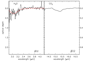
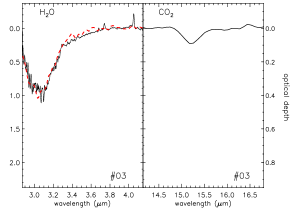
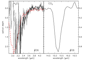
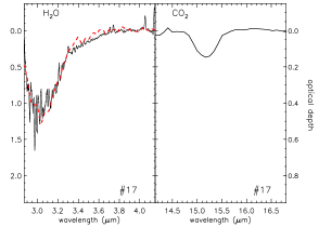
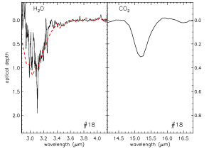
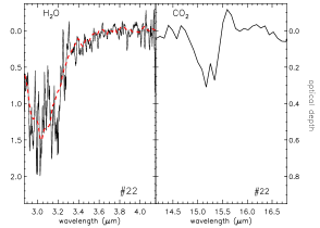
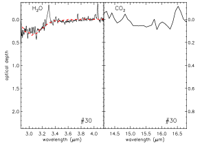
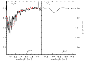
Figure 4: SMC sources with H₂O ice (left) and CO₂ ice (right) detections. Dashed (red) lines show a low-resolution AKARI spectrum of a LMC YSO (Shimonishi et al., 2010) to help constrain the blue wing of the H₂O ice feature. Source #30 shows H₂O ice but not CO₂ ice. Many sources show hydrogen emission at 3.74 $\mu$m (Pf$\gamma$) and 4.05 $\mu$m (Br$\alpha$); sources #02 and 30 exhibit PAH emission at 3.3 $\mu$m, and #06 and 30 at 16.45 $\mu$m. Source #22 shows [Ne iii] emission at 15.6 $\mu$m.

Figure 5: continued

The H₂O ice detection for source #33 is marginal. The CO₂ ice detection for source #34 is weak but significant.

Figure 6: Additional SMC sources with CO₂ ice detections. No 3$-$4 $\mu$m spectrum is available for these sources. The CO₂ ice profile of source #21 is distorted by a couple of pixels with large errors, shifting the peak position.

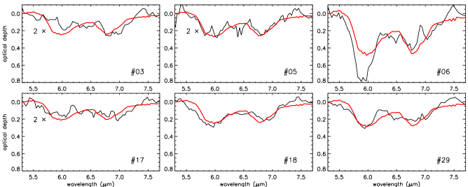
Figure 7: SMC sources with ice detections in the 5$-$7 $\mu$m range. This band is attributed to H₂O ice at 6 $\mu$m with smaller contributions from more complex molecules (HCOOH, H₂CO and NH₃), and ammonium (NH${}_{4}^{+}$) with a small contribution from methanol (CH₃OH) at 6.85 $\mu$m (Boogert et al., 2008). This ice complex can only be clearly identified when the 6.22-$\mu$m PAH feature is weak or absent. Some optical depth spectra are multiplied by a factor 2 (as indicated) to improve feature visibility. The red line is an optical depth spectrum of a Galactic YSO for comparison (Zasowski et al., 2009).

In cold molecular clouds, layers of ice form on the surface of dust grains. H₂O is by far the most abundant ice (typically $10^{-5}-10^{-4}$ with respect to H₂), followed by CO₂ and CO, with a combined abundance of 10$-$30% with respect to H₂O ice (e.g., van Dishoeck, 2004). Understanding ice chemistry is crucial to understanding the gas-phase chemistry and to probing the physical conditions within molecular clouds. Surface chemistry and UV and cosmic-ray processing of the ice mantles are thought to play an important role not only in the formation of more complex ice species but also H₂O, O₂ and gas-phase organic molecules. Prominent ice features in the IRS spectral range are found between 5 and 7 $\mu$m (attributed to a mixture of H₂O, NH₃, CH₃OH, HCOOH and H₂CO ices, e.g., Boogert et al. 2008), and at 15.2 $\mu$m (attributed to CO₂ ice, e.g., Gerakines et al. 1999; Pontoppidan et al. 2008). The ice complex at 5$-$7 $\mu$m can be difficult to identify due to the superposition of numerous PAH emission features (Spoon et al., 2002). At shorter wavelengths, ice features of H₂O and CO are found in the 3$-$5 $\mu$m range (e.g., Oliveira et al., 2011). Circumstellar ices have been detected in massive YSO environments in the Galaxy (e.g., Gerakines et al., 1999; Gibb et al., 2004) and the LMC (van Loon et al., 2005, 2008; Oliveira et al., 2009, 2011; Seale et al., 2011; Shimonishi et al., 2010).

In the SMC, H₂O and CO₂ ices (at 3 $\mu$m and 15.2 $\mu$m respectively) have been detected in the environments of sources #03, 17, 18, 32 and 34 (van Loon et al., 2008; Oliveira et al., 2011). Even though CO ice at 4.67 $\mu$m is detected towards YSOs in the Galaxy and the LMC (Gibb et al., 2004; Oliveira et al., 2011), no CO ice is detected towards sources #03, 17, 18, 33 and 34 (the only SMC sources observed at relevant wavelengths). Oliveira et al. (2011) interpreted this as a metallicity effect. Sources #03, 06 and 17 exhibit a broad feature between 60$-$70 $\mu$m in the MIPS-SED spectrum, attributed to crystalline H₂O ice (van Loon et al., 2010b).

In this work we newly identify ice features towards a number of SMC YSO candidates. We detect H₂O and CO₂ ice absorption in the environments of sources #02, 05, 06, 22 and 29 (Figs. 4, 6 and 7). For sources #05 and 29 we do not have 3$-$4 $\mu$m spectra to probe the strongest 3-$\mu$m H₂O band, but we detect the 6-$\mu$m H₂O band — also identified in sources #03, 06, 17 and 18 (Fig.7). Additionally we detect only CO₂ ice towards sources #08, 13 and 21 (Fig. 6); no 3-$\mu$m spectra are available and no ice is detected at 5$-$7 $\mu$m due to the presence of strong PAH emission (Table 3).

The blue edge of the 3-$\mu$m H₂O ice feature is set by the Earth’s atmospheric cut-off. Therefore we use the sources’ $K_{\rm s}$-band magnitudes to help constrain the continuum bluewards of the feature; the red continuum is constrained avoiding hydrogen emission at 3.74 $\mu$m (Pf$\gamma$) and 4.05 $\mu$m (Br$\alpha$). For the CO₂ ice we use a narrow wavelength interval surrounding the feature to constrain the continuum. Optical depth spectra are determined by subtracting a polynomial fitted to this local pseudo-continuum from each spectrum.

The L-band spectrum of source #06 is very red and the signal-to-noise ratio in the blue wing of the 3-$\mu$m H₂O feature is poor. Therefore we do not measure the column density directly from the ISAAC spectrum. Instead we scaled a low-resolution AKARI spectrum of a LMC YSO (SSTISAGE1C J051449.41$-$671221.5, Shimonishi et al., 2010) to match the red wing of the feature in #06 (as shown in Fig. 4), and measure the column density of the scaled spectrum. This measurement is indicated by $*$ in Table 2. We validate this technique by checking that for the other sources the two methods provide consistent column density measurements. The H₂O column density measurements for sources #02 and 30 are uncertain, since the detection is weak and PAH emission at 3.3 $\mu$m fills-in the red wing of the feature. For source #33 the H₂O ice detection is very tentative (4-$\sigma$ detection); we do not consider it any further.

The 6-$\mu$m H₂O ice feature is very complex; the contributions from other ice species can lead to overestimates of the H₂O column density (see discussion in Oliveira et al., 2009, and references therein). Therefore we do not measure the H₂O ice column density directly from the 6-$\mu$m feature. Since the peak optical depth $\tau_{6}$ correlates with the column density, we use the $\tau_{6}$ measurements and the column densities derived from the 3-$\mu$m feature for sources #03, 06, 17 and 18 to estimate the H₂O column densities for sources #05 and 29 (assuming a simple linear correlation). These measurements are indicated by $**$ in Table 2.

Table 2: Column density measurements (in $10^{17}$ molecules cm^-2) for H₂O and CO₂ ices in SMC YSO candidates. For source #06 the H₂O column density measurement (indicated by $*$) was performed by scaling a better quality spectrum (see text). For sources #05 and 29 H₂O column densities (indicated by $**$) are estimated from the 6-$\mu$m feature, rather than the 3-$\mu$m feature (see text).

source #	N(H2O)	N(CO2)
02	7.2$\pm$ 2.2	1.6$\pm$0.2
03	17.7$\pm$ 0.7	1.7$\pm$0.1
05	**19 $\pm$ 5	7.3$\pm$0.9
06	*46.3$\pm$ 7	19.2$\pm$0.5
08		2.3$\pm$0.2
13		2.2$\pm$0.2
17	21.6$\pm$ 0.8	2.8$\pm$0.1
18	22.3$\pm$ 1.2	6.0$\pm$0.2
21		3.0$\pm$0.3
22	27.7$\pm$ 3.3	6.0$\pm$1.0
29	**32 $\pm$ 5	6.7$\pm$0.1
30	4.9$\pm$ 1.0	$<$ $\sim$ 2
32	18.8$\pm$ 1.5	1.5$\pm$0.2
33	3.9$\pm$ 1.0	$<$ $\sim$ 0.3
34	16.6$\pm$ 0.7	1.0$\pm$0.2

The red wing of the CO₂ ice feature for sources #08 and 22 is affected by weak [Ne iii] emission at 15.6 $\mu$m (see next subsection). Weak H₂O ice is detected towards source #30 but no CO₂ ice is identified (an upper limit is listed in Table 2). The CO₂ ice detection towards source #34 is weak but significant, since clear H₂O ice is detected. For source #33 no CO₂ ice is detected.

Calculated ice column densities are listed in Table 2. The adopted band strengths are $2.0\times 10^{16}$ and $1.1\times 10^{17}$ cm² per molecule, respectively for H₂O and CO₂ (Gerakines et al., 1995). The quoted uncertainties for measurements in Table 2 do not reflect uncertainties in continuum determination. We have re-calculated CO₂ column densities for sources #03, 17, 18 and 34 using optimally extracted IRS spectra (Oliveira et al. 2011 used tapered-column extraction spectra; the optimal spectra provide better feature contrast due to improved signal-to-noise ratio). Sources with stronger ice absorption tend to be the most embedded (as measured by the spectral index), as observed also in Galactic samples (see for instance Forbrich et al., 2010). However, a steep spectral index does not imply the presence of ice absorption. There is weak anti-correlation between ice column density and the source luminosity.

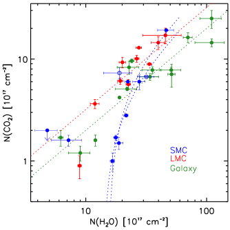
Figure 8: Column densities for H₂O and CO₂ ices. Red and green filled circles represent respectively LMC and Galactic YSOs; the dashed red and green lines represent the estimated N(CO₂)/N(H₂O) ratios, respectively 0.32 and 0.2 (Oliveira et al., 2011, and references therein). SMC measurements are represented by blue circles. Two fits to the SMC data, of the type $N({\rm CO}_{2})=m\times N({\rm H}_{2}{\rm O})+N_{0}({\rm H}_{2}{\rm O})$ ($m$ is the slope and $N_{0}({\rm H}_{2}{\rm O})$ is the H₂O column density threshold), are shown (blue dashed lines), including and excluding the 6-$\mu$m H₂O measurements (open blue circles).

Oliveira et al. (2011) compared the column densities for H₂O and CO₂ ices for Galactic and LMC samples. They found $N$(CO₂)/$N$(H₂O) ratios for the LMC and the Galaxy $\sim 0.32$ and $\sim 0.2$ respectively, consistent with previous determinations. For the SMC, rather than a constant ratio, Fig. 8 suggests that there is a H₂O column density threshold for the detection of CO₂ ice, something not observed in either the LMC or the Galaxy. Source #02 is the only SMC source with $N$(H₂O) $<1\times 10^{18}$ cm^-2 and a CO₂ ice detection, and as explained above $N$(H₂O) may be underestimated for this source. We perform linear fits to the SMC data, of the form $N({\rm CO}_{2})=m\times N({\rm H}_{2}{\rm O})+N_{0}({\rm H}_{2}{\rm O})$ where $m$ is the slope and $N_{0}$(H₂O) is the H₂O ice column density threshold for the detection of CO₂ ice. Excluding sources #02 (see above) and #30 (upper limit), the fitted slope is $\sim 0.4-0.6$ and $N_{0}$(H₂O) $\sim 1.4-1.55\times 10^{18}$ cm^-2 (depending on whether the 6-$\mu$m H₂O measurements are included, open blue circles in Fig. 8).

In the LMC, CO₂ ice column densities are enhanced with respect to H₂O ice, while the relative CO-to-CO₂ abundances are unchanged. CO₂ production could be increased due to the stronger UV field and/or higher dust temperatures in the LMC. However such harsher conditions would also destroy CO ice (the most volatile ice species), something that is not observed. Instead Oliveira et al. (2011) suggest that H₂O ice is depleted due to the combined effects of a lower gas-to-dust ratio and stronger UV radiation field. This would push the onset of water ice freeze-out deeper into the YSO envelope therefore reducing the observed column density (see their Figure 3). Forming deeper in the YSO envelope, CO₂ ice would remain unaffected.

In the Galaxy, the $A_{\rm V}$-thresholds for the detection of H₂O and CO₂ ices are statistically indistinguishable (see Oliveira et al., 2011, and references therein), suggesting that the two ices species are co-spatial in YSO envelopes. However, in the SMC the present observations suggest a column density threshold $N_{0}$(H₂O) $\sim 1.5\times 10^{18}$ cm^-2 for the detection of CO₂ ice; even the LMC measurements are consistent with a small threshold $N_{0}$(H₂O) $\sim 3\times 10^{17}$ cm^-2. This suggests that in metal-poor environments part of the envelope may have H₂O ice but not CO₂ ice, supporting the scenario proposed by Oliveira et al. (2011). The role of reduced shielding in regulating the ice chemistry mentioned above is also supported by the non-detection (with high confidence) of CO ice absorption in the spectra of five SMC sources (the only sources observed at 4.67 $\mu$m).

4.3 PAH and fine structure emission

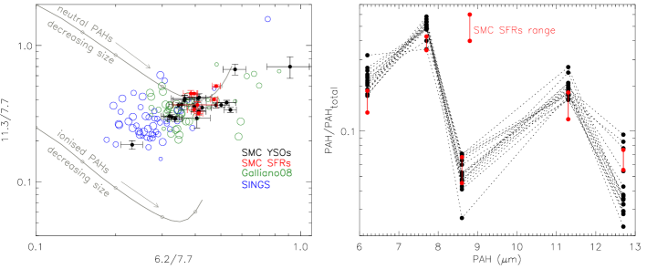
Figure 9: PAH properties towards SMC sources. Left: 11.3/7.7 intensity ratio against 6.2/7.7 ratio. The different samples are: SMC YSO candidates (this work, filled black circles), SMC SFRs (Sandstrom et al., 2012, filled red circles), a sample of galaxies and individual SFRs (Galliano et al., 2008, green circles) and finally the SINGS galaxies (Smith et al., 2007, blue circles). Symbol sizes represent three metallicity ranges: $12+\log(\rm{O/H})=7.7-8.2$, $8.2-8.7$, and $8.7-9.2$ dex. Solid grey lines indicate model trends for neutral and ionised PAHs of varying grain sizes adapted from Draine & Li (2001). Right: PAH intensity carried in each band normalised to total PAH intensity.

Numerous emission features originate from the C–C and C–H stretching and bending modes of PAH molecules, excited by UV radiation. The best studied emission bands are at 6.2, 7.7, 8.6, 11.3 and 12.7 $\mu$m, ubiquitous in the spectra of compact H ii regions and planetary nebulae. Many sources also exhibit a PAH emission complex at 17 $\mu$m. Often these emission bands are accompanied by fine-structure emission lines such as [S iv] at 10.5 $\mu$m, [Ne ii] at 12.8 $\mu$m, [Ne iii] at 15.6 $\mu$m, [Si ii] at 34.8 $\mu$m, and [S iii] at 18.7 and 33.5 $\mu$m. These lines (unresolved in the low-resolution IRS modes) originate from ionised gas. The presence of both PAH and fine-structure line emission clearly suggests the presence of an ionising source of UV radiation.

In the sample of 34 objects, all but two exhibit PAH emission. Even when other PAH bands are weak, the relatively isolated 11.3-$\mu$m band can be easily identified. Thus we use the relative peak strength of this feature to assess how dominant PAH emission is in shaping the IRS spectrum. We fit a local continuum using spectral points to the left and right of the feature, and measure the peak strength of the feature with respect to the underlying continuum, $F_{11.3}/F_{c}$. Sources with $F_{11.3}/F_{c}\leq 1.05$ essentially show no PAH emission; this is the case of sources #18 and 19. For sources with $1.05<F_{11.3}/F_{c}\leq 1.30$ only the 11.3-$\mu$m band can be easily identified, other bands are not clearly visible (typical examples are sources #03 and 20). Sources with $F_{11.3}/F_{c}>1.3$ clearly exhibit the complete zoo of PAH features (e.g., #08), and for some sources the spectra are completely dominated by PAH emission ($F_{11.3}/F_{c}>3$, e.g., #07). The different PAH groups are listed in Table 3 as ✕, ✓, ✓, ✓✓ from absent to very strong, and are used in the source classification in Section 5.

Recently, Sandstrom et al. (2012) analysed the properties of PAH emission observed towards a sample of six diverse star forming regions (SFRs) in the SMC, namely N76 and N66 in the northeast SMC bar, three regions in the southwest bar including N22, and N83/84 in the SMC Wing. Our sample comprises sources in the same six regions, and further extends the spatial coverage by sampling for instance the region in the SMC body that connects N 66 to the southwest bar (see Fig. 1). Fig. 9 summarises PAH properties in the SMC. On the left we show intensity ratios for the YSO candidates (black filled circles) and the averages for the aforementioned SMC SFRs (red filled circles). On the right we show the intensity of each main band normalised to total PAH intensity. In our sample the 11.3-$\mu$m band is strong compared to the 7.7- and 6.2-$\mu$m bands, and the 8.6-$\mu$m band is very weak compared to total PAH strength, consistent with the Sandstrom et al. (2012) results. Our analysis does not reveal changes to PAH emission properties that would be evidence for the YSO’s irradiation of its environment. Thus the PAH emission observed towards at least some YSO candidates may have an important environmental contribution. Nevertheless, for sources with strong emission, total PAH intensity correlates with the luminosity of the source.

Model PAH band ratios (adapted from Draine & Li, 2001, as described by Sandstrom et al. 2012) show the regions of the ratio diagram occupied by neutral and ionised PAHs, indicating also the effect of decreasing grain size. The strength of the radiation field also has a slight effect on PAH ratios. As proposed by Sandstrom et al. (2012), the comparison with these models suggests that SMC PAHs are predominantly small and neutral.

By comparing PAH properties in the SMC and the high-metallicity SINGS galaxies (Smith et al., 2007), Sandstrom et al. (2012) explain the observed differences as a metallicity effect: they speculate that, in the metal-poor SMC, PAHs form preferably in smaller grains and mostly neutral PAHs survive in the ISM. To further investigate whether the observed PAH ratios are directly related to metallicity we extend the comparison to also include the measurements compiled by Galliano et al. (2008) for a diverse sample of galaxies and individual SFRs of a range of metallicities. These data are show in Fig. 9 (left): the SINGS and Galliano samples are represented by open blue and green circles respectively, and the symbol size reflects each region’s gas-phase oxygen abundances, in the intervals $12+\log(\rm{O/H})=7.7-8.2$, $8.2-8.7$, and $8.7-9.2$. We adopt $12+\log(\rm{O/H})=8.0$ for the SMC. Both the SINGS and Galliano samples cover a similar metallicity range, with the majority of objects in each sample above 8.3 and 8.8 dex respectively. However, these two samples occupy different regions in the PAH ratio diagram (with some overlap) despite their similar metallicities. The SMC measurements sit in a similar region to the Galliano sample, despite its lower metallicity. In summary our analysis supports the suggestion that PAHs throughout the whole SMC are indeed predominantly small and neutral; however the sample comparisons we describe do not support a simple metallicity explanation; other global environmental parameters should also play a role (e.g., Haynes et al., 2010).

Fine-structure emission from atomic ions can be intrinsic to YSO sources but it can also be a result of contamination from the diffuse gas or nearby H ii regions. Furthermore, at this resolution, it is difficult to separate from PAH emission, particularly for the 12.8-$\mu$m [Ne ii] line. While the IRS spectra of 8 objects exhibit the 18.7- and 33.5-$\mu$m [S iii] emission lines (Table 3), only sources #26 and 31 show strong 8.99-$\mu$m [Ar iii], 10.5-$\mu$m [S iv] and 15.6-$\mu$m [Ne iii] emission lines, also present but weaker in the spectra of #08 and 22. Spectral contamination from the environment is likely given the location of many targets in the vicinity of known H ii regions (Fig. 1 and further discussion in Section 5.1).

4.4 H₂ emission

H₂ emission is expected to be ubiquitous in YSO environments. However, only when the molecular gas is heated to a few hundred K is H₂ emission observable. Both UV radiation (released by the accretion process, the emerging star itself, or from nearby environment) and shocks (created as outflows interact with the quiescent molecular cloud) can produce warm H₂ gas (for a review see Habart et al., 2005). Extinction-corrected excitation diagrams can be used to diagnose the gas conditions and constrain the excitation mechanism of massive YSOs (e.g., van den Ancker, Tielens & Wesselius, van den Ancker et al.2000).

Several emission lines due to molecular hydrogen are included in the IRS range. In particular pure-rotational $0-0$ transitions occur at 5.51 S(7), 6.10 S(6), 6.91 S(5), 8.03 S(4), 9.66 S(3), 12.28 S(2), 17.03 S(1) and 28.22 $\mu$m S(0). The S(6) and S(4) transitions are difficult to disentangle from the PAH emission, the S(5) line can be contaminated by [Ar iii] at 6.99 $\mu$m, and the S/N ratio in the region of the S(7) line is sometimes low. Nevertheless we have identified H₂ emission in the spectra of the majority of objects in our sample: for 24 sources three or more unblended emission lines are measured (✓ in Table 3), while for eight sources only two weak lines are identified (✓? in Table 3). There are two sources with no detectable H₂ emission lines (✕ in Table 3).

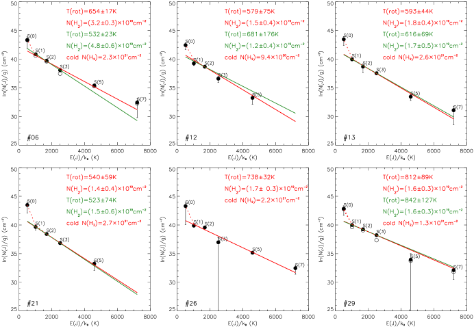
Figure 10: H₂ excitation diagrams for selected SMC YSO candidates. For sources #06 and 29, the line intensities are corrected for extinction (see text for details). The results of two fits are displayed when available: a fit to all measured lines (red), or a fit to only S(1) to S(3) (green). For each fit, the derived rotational temperature $T_{\rm rot}$ and column density $N({\rm H_{2}})$ are indicated. The dashed red line shows the contribution of a cold H₂ component, with fixed temperature $T_{\rm rot}=100$ K.

Since the lines discussed here are optically thin (Parmar, Lacy & Achtermann, 1991), the measured line intensities can be used to derive the total number of molecules and the rotational temperature. For excited H₂ gas in local thermodynamic equilibrium (LTE) at a single temperature, the density $N(\rm{H_{2}})$ and temperature $T_{\rm rot}$ are described by the Boltzmann distribution (in logarithmic form):

$$\ln\left(\frac{N(J)}{g_{J}}\right)=-\frac{E(J)}{k_{B}\,T_{\rm rot}}+\ln\left(N(H_{2})\frac{h\,c\,B}{2\,k_{B}\,T_{\rm rot}}\right)$$ (1)

where $g_{J}$, $E(J)$ and $N(J)$ are respectively the statistical weight, energy and column density of the upper $J$ level , $B=59.33$ cm^-1 is the H₂ molecular constant. The statistical weight is given by $g_{J}=g_{S}(2J+1)$, where the nuclear spin weight $g_{S}=3$ for $ortho$-states (odd $J$) and $g_{S}=1$ for $para$-states (even $J$) — we assume an equilibrium ortho-to-para ratio $opr=3$, appropriate for gas with $T>300$ K (e.g., Sternberg & Neufeld, 1999). The column density $N(J)$ is derived from the measured extinction-corrected line intensities $I(J)$ as follows:

$$N(J)=4\,\pi\,\frac{\lambda}{h\,c}\frac{I(J)}{A_{J}\Omega}$$ (2)

where $A_{J}$ are the transition probabilities and $\Omega$ is the beamsize in steradian. More details on the method and values of relevant constants and energies can be found in the literature (e.g., Parmar et al., 1991; Bernard-Salas & Tielens, 2005; Barsony et al., 2010).

To estimate the beamsize $\Omega$ we multiply the FWHM of the PSF by the slit width. Slit widths are $3\hbox to0.0pt{.\hss}^{\prime\prime}6$ and $10\hbox to0.0pt{.\hss}^{\prime\prime}6$ respectively for SL and LL. The FWHM is measured from the two-dimensional PSF as a function of wavelength, ranging from $1\hbox to0.0pt{.\hss}^{\prime\prime}9$ at 5.51 $\mu$m to 7^′′ at 28.2 $\mu$m. The PSFs are those used for the optimal extraction of the spectra (Section 3.1 and Lebouteiller et al., 2010). We choose to have a beamsize that increases with wavelength since some objects are marginally resolved, and in such complex environments at these large distances, the IRS spectra do sample different sized emission regions.

To estimate the extinction, we use pahfit (Smith et al., 2007) since it disentangles the contributions from the dust and PAH emission; the code returns fully mixed relative extinctions that can be used to correct the observed line intensities. The extinction corrections are largest for the S(3) 9.66-$\mu$m line, but still usually small for the targets in the present sample.

Figure 10 shows examples of H₂ excitation diagrams for several SMC sources, open and full circles represent respectively uncorrected and extinction-corrected measurements. For each object with more than two H₂ emission line measurements a straight line can be fitted to the data points, allowing the determination of the temperature and column density, using Eq. (1). It can be seen from the examples in Fig. 10 that the weighted column density for S(0) is always high compared to the measurements for other lines. This is to be expected since S(0) has the lowest energy, therefore it probes the reservoir of H₂ that is too cool to excite any other transitions. We discuss S(0) emission later.

Whenever possible we perform two fits; the first makes use of all good measurements available except S(0), the second makes use only of S(1), S(2) and S(3) (red and green lines in Fig. 10 respectively). The reason to perform the second fit to the three transitions closest in energy level is to investigate possible deviations from the simple single temperature scenario, as it could be expected if a smaller column of hotter H₂ is also present (, van den Ancker et al.2000). In general, a single-temperature Boltzmann distribution provides good fits to the weighted column densities within the measurement uncertainties. Firstly this validates the adopted wavelength-dependent beamsizes, rather than a single beamsize. Furthermore the column density of the S(2) line, the only $para$-state we are able to measure, does not deviate from those of the $ortho$-states, suggesting that the adopted LTE value of $opr=3$ is adequate. The two fits described above (see examples in Fig. 10) result in temperatures that agree within 1.5$\sigma$ for all objects except for source #06 (5-$\sigma$ difference). This again shows that a single temperature fit is appropriate to describe the molecular gas responsible for most of the emission. The exception is source #06, for which the excitation diagram and fitted temperatures suggest the presence of a hotter H₂ contribution (top left panel in Fig. 10).

For the fits to 4 or 5 data points the median temperature is $T_{\rm rot}=594\pm 99$ K (range $439-812$ K), while for the 3-measurement fits the median temperature is $T_{\rm rot}=562\pm 100$ K (range $439-843$ K). The median densities are respectively $N({\rm H_{2}})=1.8\pm 0.9\times 10^{19}$ cm^-2 (range $0.6-3.8\times 10^{19}$ cm^-2) and $N({\rm H_{2}})=1.6\pm 1.5\times 10^{19}$ cm^-2 (range $0.7-4.8\times 10^{19}$ cm^-2). When compared to a sample of Galactic YSOs (van den Ancker, 1999) covering the same luminosity range, the rotational temperatures are similar. However, the column densities for the SMC YSO candidates tend to be smaller by a factor three, typically $\sim 1.7\times 10^{19}$ cm^-2 rather than $\sim 5\times 10^{19}$ cm^-2.

Neither H₂ temperature or column density seem correlated with source luminosity for the SMC and Galactic samples. For sources with strong PAH emission, H₂ intensity (using S(3) as a proxy) is largest for sources with the largest total PAH intensity. However, there is no distinction between the derived H₂ properties for sources with ice and silicate absorption, and PAH emission. Since, as discussed in the next section, these features trace the YSO evolution, this implies that H₂ emission does not seem to correlate with evolutionary stage, neither in SMC nor Galactic samples (see also Forbrich et al., 2010).

As already mentioned, the weighted column density for S(0) is too large when compared to the other transitions, suggesting a reservoir of quiescent cold gas. Since this cold component is poorly constrained, we opt to fix its temperature at 100 K (e.g., Lahuis et al., 2010) and simply adjust the column density to match the observed $N(0)/g(0)$. We do not constrain $opr$, expected to be $\sim 1.6$ for this temperature (Sternberg & Neufeld, 1999). The contribution of this cold component, added to the main warm component, is shown in Fig. 10 (dashed red line). The fitted column densities are in the range $N({\rm H_{2}})=0.4-3.8\times 10^{21}$ cm^-2 (median density $2.3\times 10^{21}$ cm^-2). Therefore the contribution of the cold molecular gas reservoir is substantial, even though its signature is only observed in the S(0) emission.

On their own the column densities and temperatures derived in this way cannot constrain the excitation mechanism: there is significant overlap in the parameter range predicted for shocked and photo-dissociated gas (Habart et al., 2005; Bernard-Salas & Tielens, 2005), even though higher temperatures are suggestive of shocked gas. Other diagnostics are available: PAH emission suggests photo-dissociated gas while [S i] emission at 25.25 $\mu$m indicates shocked gas. As already discussed, the majority of the sources in the sample exhibit PAH emission. We do not detect the [S i] line in any of the spectra. Even though it is likely that both mechanisms contribute to H₂ excitation, the available evidence suggests that radiation is the dominant excitation mechanism in these SMC sources. Since H₂ emission is also excited in photo-dissociation regions (e.g., Habart et al., 2005), it is possible that there is an environmental contribution to emission observed towards the YSO candidates. This may be true in particular for the warmer component, the cool component originating from the denser more shielded regions.

4.5 Optical spectra

In this section we discuss the optical emission-line spectra of 20 SMC sources — for the remaining 14 sources either no optical spectrum could be obtained, the spectrum is not associated with the IR source, or only H$\alpha$ emission is detected (Section 3.5.1). In H ii regions and their precursors surrounding young massive stars, common optical emission lines are due to permitted hydrogen (Balmer and Paschen) and O i emission (8446 Å) and numerous forbidden emission lines: [O i] (6300 Å), [O ii] (3727, 7322, 7332 Å), [N ii] (6548, 6583 Å), [S ii] (6717, 6731 Å), as well as [O iii] (4363, 4959, 5007 Å) and [S iii] (9068, 9530 Å). If the object is massive enough (early O-type source) an appreciable He⁺ ionisation zone develops (e.g., Draine, 2011) and He i recombination emission is detected (at 3888, 4471, 5875, 6678, 7065 Å). Hydrogen emission in YSOs originates both from the accretion columns and outflows. Forbidden line emission can also originate in the relatively low-density environments of outflowing jets or winds (e.g., White & Hillenbrand, 2004) but it is also observed in PDR-like environments (Störzer & Hollenbach, 2000). Velocity information can distinguish between the two excitation scenarios (e.g., Störzer & Hollenbach, 2000) but our spectra have insufficient velocity resolution (e.g., $\sim 205$ km s^-1 at the position of H$\alpha$).

Figure 4 shows the optical spectra of the 32 SMC sources; the last panel shows the rich spectrum of source #26 with the emission lines identified. We implement a classification scheme that relies on the detection of progressively higher excitation energy emission lines. Thus the classification reflects the harshness of the near-YSO environment. Type I objects exhibit emission from the Balmer and Paschen series and O i, Type II objects add collisionally excited lines of [O ii], [N ii] and [S ii]. Type III objects exhibit also [O iii] emission, Type IV objects add [S iii], and finally Type V objects show prominent He i recombination emission. The type breakdown of the sample of twenty sources is as follows: two Type I, two Type I/II (only H$\alpha$ and [S ii] emission, see below), four Type II, one Type III, two Type IV, four Type IV/V (a single He i line identified), and four Type V; the optical spectrum of source #19 is discussed in Section 5.

Of the ten sources classified as Type IV or V, all sources exhibit PAH emission and seven show IR fine-structure emission. Most are also detected at radio wavelengths (see Table 3). Conversely, all the objects that show IR fine-structure emission, and for which we have an optical spectrum, are classified as Type IV$-$V. These ten sources have the highest luminosities ($L\,{\vbox{\hbox{$>$}\offinterlineskip\hbox{$\sim$}}}\,10^{4}\,L_{\odot}$), as determined from SED fits (Table 3). This builds a consistent picture of these objects representing more evolved YSO candidates, i.e. ultracompact H ii regions. However, four of these sources do exhibit ice features in their IRS spectrum (see next section), suggesting deeply embedded objects.

As mentioned above the optical spectra do not have enough resolution to investigate the origin of the emission features. However, we have looked for broadening of the line profiles that would indicate infall and/or outflow activity. In fact, a number of sources show evidence of broadened H$\alpha$ profiles: 13 sources (indicated in Table 3) have FWHM in the range 300$-$440 km s^-1. Furthermore, two sources (#32 and 33) exhibit extremely broad profiles (FWHM$>600$ km s^-1) with line centroids shifted to $\sim-200$ km s^-1. These two sources are classified as Type I/II, since besides H$\alpha$ only [S ii] emission is detected (equally broad). The profiles clearly suggest an origin in optically thick winds in the environments of these two YSO candidates.

5 Source classification

Table 3: Detailed properties of SMC YSO candidates. We use the IRS spectra to investigate PAH, fine-structure and H₂ emission and silicate absorption/emission, and calculate the spectral index between 3.6 and 24 $\mu$m. The presence or absence of a feature is indicated by ✓ and ✕, ? indicating doubt (see discussion in the text). For PAH emission the contrast of the 11.3-$\mu$m feature with respect to the continuum is analysed in more detail: ✓✓, ✓, ✓ indicate very strong, strong and weak emission respectively (see text). Four objects with silicate emission are identified with $\bigwedge$. For H₂ emission, ✓? indicates objects for which only two emission lines were detected, rather than three to five. Ice species investigated are H₂O (at 3.1, 6 and 60 $\mu$m), CO (4.67 $\mu$m) and CO₂ (15.2 $\mu$m). The optical ionisation classes are defined according to the emission lines present in the spectrum: Type I objects exhibit Balmer, Paschen and O i, Type II objects show hydrogen, O i, [N ii], [O ii] and [S ii] emission, Type III objects show the same lines plus [O iii], Type IV objects further add [S iii], and finally Type V objects show all these lines plus He i emission. Some objects exhibit a stellar absorption spectrum and others only H$\alpha$ in emission (see text for discussion). Objects that exhibit H$\alpha$ emission broader than 300 km s^-1 are also indicated. The next column indicates whether the object has been detected at radio wavelengths; $*$ signals an extended source. The sources are classified using features in their IRS spectrum, according to two classification schemes previously applied to samples of LMC YSOs (Seale et al., 2009; Woods et al., 2011). The last column provides the luminosities determined from the SED fits. All sources are classified as YSOs (Section 5), except for source #19 that is a D-type symbiotic system (Section 6).

#	PAH	silicate	H2	fine struct.	$\beta$	H2O ice			CO ice	CO2 ice	optical	broad	radio	YSO class.		$L$
	emission		emission	emission	3.6$-$24$\mu$m	3 $\mu$m	6 $\mu$m	60 $\mu$m	4.67$\mu$m	15.2$\mu$m	Type	H$\alpha$	source	S09	W11	$(10^{3}$L${}_{\odot})$
01	✓	✕	✓	✓	$-$2.6		✕			✕	IV/V	n	y	PE	G3	16
02	✓	✓	✓	✕	$-$2.4	✓	✕	✕		✓	only H$\alpha$ emission	y	y	S	G1	19
03	✓	✓	✓?	✕	$-$2.2	✓	✓	✓	✕	✓	V	n	y	S	G1	61
04	✓	✕	✓	✕	$-$1.6		✕			✕	II	y	n	P	G3	2.3
05	✓	$\bigwedge$	✓	✕	$-$1.5		✓			✓	absorption lines		n	O	G1	1.6
06	✓	✓	✓	✕	$-$2.2	✓	✓	✓		✓	absorption lines		n	S	G1	5.8
07	✓✓	✕	✓	✕	$-$1.7		✕			✕	II	n	n	P	G3	4.2
08	✓	✕	✓	✓	$-$3.0		✕			✓	V	n	y∗	PE	G1	1.9
09	✓	✕	✓	✓	$-$2.5		✕			✕	IV/V	n	y	PE	G3	7.9
10	✓	✕	✓	✕	$-$3.0		✕			✕	only H$\alpha$ emission	y	y	P	G3	33
11	✓✓	✕	✓	✕	$-$1.8		✕			✕	only H$\alpha$ emission	y	n	P	G3	2.2
12	✓✓	✕	✓	✕	$-$2.5		✕			✕	III	n	n	P	G3	2.3
13	✓	✕	✓	✓	$-$3.1		✕			✓	IV	n	n	PE	G1	22
14	✓	$\bigwedge$	✓?	✕	$-$2.1		✕			✕	only H$\alpha$ emission	y	n	O	G4	1.8
15	✓	✕	✓	✓	$-$3.1		✕			✕	V	n	y∗	PE	G3	21
16	✓	✕	✓	✕	$-$3.1		✕			✕	only H$\alpha$ emission	y	n	P	G3	12
17	✓	✓	✓?	✕	$-$1.7	✓	✓	✓	✕	✓	only H$\alpha$ emission	y	n	S	G1	22
18	✕	✓	✕	✕	$-$2.2	✓	✓	✕	✕	✓	only H$\alpha$ emission	y	n	S	G1	28
19	✕	$\bigwedge$	✕	✕	$-$3.2		✕			✕	III-V	y	n	not a YSO		34
20	✓	$\bigwedge$	✓?	✕	$-$1.8		✕			✕	I	y	n	O	G4	1.5
21	✓	✕	✓	✕	$-$2.9		✕			✓	II	n	n	P	G1	11
22	✓	✕	✓	✓	$-$2.2	✓	✕			✓	IV/V	y	n	PE	G1	9.1
23	✓✓	✕	✓	✕	$-$2.9		✕			✕	only H$\alpha$ emission	n	n	P	G3	14
24	✓	✓?	✓	✕	$-$1.5		✕			✕	no spectrum		n	P	G2/G3	4.5
25	✓	✕	✓	✕	$-$2.8		✕			✕	IV	n	y	P	G3	17
26	✓	✕	✓	✓	$-$2.3		✕			✕	V	n	y	PE	G3	12
27	✓✓	✕	✓	✕	$-$2.6		✕			✕	II	n	n	P	G3	3.3
28	✓	✓	✓?	✕	$-$2.7	✕	✕	✕		✕	IV/V	n	y	S	G2	140
29	✓	✓	✓	✕	$-$2.7		✓			✓	absorption lines		n	S	G1	10
30	✓	✓?	✓	✕	$-$1.0	✓	✕	✕		✕	I	y	n	P	G1	7.9
31	✓	✕	✓?	✓	$-$2.7		✕	✕		✕	no spectrum		y∗	PE	G3	6.7
32	✓	✓	✓	✕	$-$1.6	✓	✕			✓	I/II	y	n	S	G1	3.5
33	✓	✓	✓?	✕	$-$1.4	?	✕	✕	✕	✕	I/II	y	n	S	G2	26
34	✓	✓	✓?	✕	$-$1.8	✓	✕	✕	✕	✓	only H$\alpha$ emission	y	n	S	G1	23

All but one of the sources in the SMC sample are YSOs, based on the IR spectral properties analysed in the previous section: ice absorption, silicate absorption or emission, PAH and H₂ emission, red continuum and SED fitting. Boyer et al. (2011) tentatively proposed that nine of these sources are very dusty evolved stars, based on Spitzer photometric criteria. Seven of those sources show ice absorption and two others show silicate absorption, and are thus clearly SMC YSOs. The only non-YSO source in our sample (#19) is discussed in Section 6.

Two YSO spectral classification schemes have been recently developed and applied to YSO samples in the LMC. Seale et al. (2009) performed an automated spectral classification of YSOs using principal component analysis to identify the spectral features that dominate the spectra; the following classes are relevant for the SMC sample: S objects show spectra dominated by silicate absorption, P and PE objects show PAH emission and IR fine-structure emission and O objects show silicate emission. There is an evolutionary sequence associated with this classification in the sense that objects with S spectra are more embedded while P and PE spectra are associated with more evolved compact H ii regions. We have classified the objects in the YSO sample using this classification scheme (Table 3).

The other classification scheme was introduced by Woods et al. (2011): objects are classified in groups depending on spectral features present in the spectrum, from G1 (ice absorption), G2 (silicate absorption), G3 (PAH emission) and G4 (silicate emission). The main difference from the Seale classification is the usage of ice absorption as a clear indicator of a very cool envelope, identifying the earliest embedded sources. Thus we discuss the classification of the SMC YSOs using this method in more detail (Table 3).

5.1 Embedded YSOs

There are fourteen SMC sources classified as belonging to group G1, i.e. exhibiting ice absorption. Most G1 sources (eight) also exhibit silicate absorption, but this is not always the case: source #05 shows a silicate emission feature (see Section 5.3), while sources #08, 13, 21, 22 and 30 show strong PAH emission that could mask weak silicate absorption — we suspect this to be the case particularly for #30. Of the aforementioned fourteen sources, ten show definite H₂ emission, three have weak H₂ emission, and one source shows no H₂ emission. Eight G1 sources have weak or no PAH emission features while six sources show strong emission (three of which also show fine-structure emission). Of the fourteen G1 sources, three have no optical spectra and seven exhibit either only H$\alpha$ or low-excitation emission lines. Another four G1 sources, namely #03, 08, 13 and 22 are classified as Type IV$-$V based on the counterpart optical spectrum; except for #03, these sources also show strong PAH and fine-structure emission.

As already mentioned the presence of ice and silicate absorption features indicates the presence of an embedded YSO while PAH, and forbidden and fine-structure emission hint at a compact H ii region. However, many sources exhibit both ice absorption and emission features. Galactic YSOs can exhibit both PAH and fine structure emission and ice absorption (e.g., W3 IRS5 and MonR2 IRS2; Gibb et al., 2004), and many LMC YSOs with CO₂ ice signatures also exhibit PAH emission (Oliveira et al., 2009; Seale et al., 2011). The same is true for the SMC sample, with half the sources exhibiting mixed-property spectra. Dust and ice features originate from the cooler regions of the embedded YSO envelope. On the other hand PAH and fine-structure emission can be excited not only by the emerging YSO itself but also by neighbouring massive stars, and more generally in the larger H ii complexes in which many YSOs reside. At the LMC and SMC distances (respectively $\sim$ 50 and 60 kpc, Ngeow & Kanbur, 2008; Szewczyk et al., 2009), it becomes impossible to disentangle the contributions of the different physical environments. The spatial resolution of a IRS spectrum varies typically from 3$\arcsec$ to 10$\arcsec$, corresponding to 1 to 3 pc in the SMC, implying that very different spatial scales are sampled at different wavelengths. This makes it difficult to use spectral features to unequivocally constrain the evolutionary stage of the object.

Nevertheless the six G1 YSOs with ice and silicate absorption, weak or absent PAH emission, no fine-structure emission and quiescent optical spectra are the more embedded, earliest YSOs (sources #02, 17, 18, 29, 32 and 34). Sources #28 and 33 (the two G2 sources) and #24 (G2/G3 source) are still relatively embedded (silicate is seen in absorption) but no ice absorption is detected, suggesting warmer envelopes. At these early stages the YSO has little influence on the physical conditions in its envelope. The remaining G1 YSOs (sources #03, 06, 08, 13, 21, 22 and 30) show both ice absorption and PAH emission in their spectra. These objects are likely more evolved since the PAH and fine-structure emission indicates that the YSO is able to emit copious amounts of UV radiation, while still retaining enough of its cold envelope responsible for the absorption features (with the possible caveat that #06, 08 and 13 sit in particularly complex environments, see Fig. 1). At this stage a (ultra-)compact H ii region is emerging.

5.2 PAH dominated YSOs

There are fourteen sources in the sample that we classify as G3, indicating that PAH emission is the noticeable feature in their steep IRS spectra. Five of the sources have fine-structure emission as well. In terms of counterpart optical spectra, there does not seem to be a strong relation between PAH emission and optical type (Section 4.5), since four sources only exhibit H$\alpha$ emission, three sources are Type II, one source is Type III and five sources are Type IV$-$V (for one further source we have no spectrum).

These fourteen G3 sources are the most evolved in the sample, with the IR spectral features clearly indicating the presence of a well developed compact H ii region, in the process of clearing out the remnant dusty envelope.

5.3 Intermediate-mass YSOs

In this subsection we discuss the three YSOs that exhibit silicates in emission in their IRS spectrum, classified as G4 (sources #14 and 20) and source #05 that also shows ice absorption. The SED of #20 is steep but flattens considerably above 20 $\mu$m. In fact, its IRS spectrum is very similar to that of the Galactic HAeBe star IRAS 04101+3103 (Furlan et al., 2006), including the weak PAH emission. A spectrum and photometry of the optical counterpart have been analysed by Martayan et al. (2007, identified as SMC5$\_037102$); they suggest that this source is a Herbig B[e] star, based on the presence of numerous Fe ii and [Fe ii] emission lines and accretion signatures in the Balmer lines. We cannot detect the iron lines in our low-resolution optical spectrum, but we confirm that H$\alpha$ is broad. The fact that the continuum flux rises from the $J_{s}$-band to 70 $\mu$m suggests that a tenuous dusty envelope remains.

The SEDs of sources #05 and 14 both have silicate emission and steep IRS spectra throughout. Source #14 shows strong PAH emission, while #05 shows weak PAH and H₂ emission as well as H₂O and CO₂ ice absorption. Furlan et al. (2008) describes a number of Galactic objects that they classify as evolved Class I YSOs; these objects still retain a low-density envelope, tenuous enough to reveal the thick accretion disc and the central star. The observed properties of sources #05, 14 and 20 suggests the same classification, with #20 the more evolved of the three sources. Note that the evolutionary scenario discussed in the previous subsection refers to massive star formation, while the present discussion addresses the evolution of intermediate-mass stars.

6 A D-type symbiotic star in the SMC

Source #19 is a clear oddity since its optical spectrum (Figs.11, 4) shows a blue continuum with broad emission lines at 6825 and 7082 Å, as well as H$\alpha$, [N ii] and [O iii] emission, with weak He i emission at 5875 and 7065 Å, and a tentative detection of He ii emission at 4686 Å. Figure 16 shows that next to the IR source there is a bright blue star. By looking at the 2-D spectrum (before extraction) we see that the continuum and emission line contributions are offset by about $2^{\prime\prime}$, in the sense that the continuum originates from the bright blue source, while the emission lines originate from the IR-bright source.

Figure 11: Detail of the optical spectrum of #19, showing the prominent Raman emission lines.

The emission features at 6825 and 7082 Å are identified as Raman scattering of the O vi resonance photons at 1032 and 1038 Å by neutral hydrogen; these lines are usually observed in the spectra of symbiotic binary systems (e.g., Schmid, 1989). Symbiotic objects are interacting binaries, in which an evolved giant transfers material to a much hotter, compact companion; according to the classification criteria of Belczyński et al. (2000), the presence of the Raman scattering lines and optical emission lines is enough to identify a symbiotic system, even if no features of the cool giant are found. Recently it has been proposed that massive luminous B[e] stars may also exhibit Raman scattering lines (Torres et al., 2012).

Source #19 has a steep SED from 2 to 20 $\mu$m (Fig. 3). Above 20 $\mu$m the IRS spectrum flattens considerably and the source becomes fainter at 70 $\mu$m. This indicates the presence of a significant amount of (not very cold) dust. It shows a prominent silicate emission feature, suggestive of unprocessed dust, and no PAH emission. This is consistent with this object being a dusty (D-type) symbiotic star (Angeloni et al., 2007). The optical spectrum shows no molecular TiO bands that would indicate the presence of the red giant. This is another common feature of D-type symbiotic stars: the reddened asymptotic giant branch star is not detected at optical wavelengths but it reveals itself at IR wavelengths (e.g., Corradi et al., 2010). In terms of photometry, source #19 has a colour $J_{s}-K_{s}\sim 1.1$ mag, and it has not been identified as variable. Given the presence of Raman scattering and H and He emission, its brightness at 70 $\mu$m, and the properties of its IRS spectrum, we propose that #19 is a D-type symbiotic system in the SMC. This adds to the six S-type (dust-less) symbiotic systems already confirmed in the SMC (Mikołajewska, 2004).

7 Summary

We present a multi-wavelength characterisation of 34 YSO candidates in the SMC. The target objects are bright in the 70-$\mu$m MIPS band, and the selection strategy aims at excluding both evolved star and bright galaxy interlopers. The basis of the analysis described here are low-resolution IR spectra obtained with Spitzer-IRS, supported by Spitzer photometry (IRAC and MIPS), near-IR photometry, 3$-$5 $\mu$m spectroscopy, low-resolution optical spectroscopy and radio data. The objective is to confirm the YSO nature of these SMC sources and characterise them. We summarise here our most important results.

• Of the 34 sources 33 are spectroscopically identified as YSOs in the SMC. This now sizable sample adds to the SMC YSOs previously identified by van Loon et al. (2008, 2010b) and Oliveira et al. (2011).

• One object (source #19) is identified as a D-type symbiotic system, based on the presence of Raman emission at 6825 and 7082 Å and nebular emission lines, as well as prominent silicate emission. This is the first D-type symbiotic identified in the SMC.

• Fourteen YSOs exhibit ice absorption in their spectra. We analyse H₂O and CO₂ ice column densities; we suggest the presence of a significant H₂O column density threshold for the detection of CO₂ ice in the SMC. The observed differences between Galactic, LMC and SMC samples can be explained as due to metallicity.

• We analyse PAH emission, which is ubiquitous in the sample. We confirm previous results from Sandstrom et al. (2012) who propose that the grains responsible for PAH emission in the SMC are mostly small and neutral. Based on the comparison of different published samples, the observed PAH properties cannot be solely determined by metallicity.

• Many objects show narrow emission lines in the IRS spectra attributed to molecular hydrogen. Excitation diagrams constrain the rotational temperature and H₂ column density of the bulk of the gas responsible to the emission. When compared to Galactic sources (van den Ancker, 1999) the rotational temperatures are similar, but the H₂ column densities in the SMC are generally smaller. Photo-dissociation is the dominant excitation mechanism. There does not seem to be a clear correlation between the detection of H₂ emission and its derived properties and the evolutionary stage of the YSO. For most sources there is also a significant reservoir of colder molecular gas ($T_{\rm rot}\sim 100$ K).

• Of the 33 YSOs in our sample, 30 cover the main stages of massive YSO evolution. Based on the presence of ice and silicate absorption and weak/absent PAH emission, six YSOs are still deeply embedded. Three other embedded sources have envelopes already too warm for significant amount of ice to survive on the dust grains. A further seven sources, while still embedded (i.e. showing IR molecular absorption features), already present evidence of an emerging H ii region. Finally, fourteen sources exhibit spectra with the hallmarks of compact H ii regions (strong PAH and fine-structure emission). Three other sources exhibit silicate emission (one shows ice absorption as well); these sources are probably sources in transition between Class I and Class II, i.e. precursors to intermediate-mass HAeBe stars that still retain a tenuous envelope.

  Scheduled ground-based observations will target more YSOs with ice signatures; column density measurements and modelling of the ice profiles will help constrain the reason for the observed differences in ice properties for samples of sub-solar metallicity. Some of the SMC YSOs are targets of an ongoing Herschel spectroscopy program that aims to constrain the role of the main cooling agents (gas-phase CO and water, OH, [C ii] and [O i]) and obtain an inventory of the species present both in gas and solid phases.

Table 4: Summary of spectroscopic observations available for the SMC sources.

#	optical	3-4$\mu$m	4-5$\mu$m	IRS	MIPS-SED
01	✓	✕	✕	✓	✕
02	✓	✓	✕	✓	✓
03	✓	✓	✓	✓	✓
04	✓	✕	✕	✓	✕
05	✕	✕	✕	✓	✕
06	✕	✓	✕	✓	✓
07	✓	✕	✕	✓	✕
08	✓	✕	✕	✓	✕
09	✓	✕	✕	✓	✕
10	✓	✕	✕	✓	✕
11	✓	✕	✕	✓	✕
12	✓	✕	✕	✓	✕
13	✓	✕	✕	✓	✕
14	✓	✕	✕	✓	✕
15	✓	✕	✕	✓	✕
16	✓	✕	✕	✓	✕
17	✓	✓	✓	✓	✓
18	✓	✓	✓	✓	✓
19	✓	✕	✕	✓	✕
20	✓	✕	✕	✓	✕
21	✓	✕	✕	✓	✕
22	✓	✓	✕	✓	✕
23	✓	✕	✕	✓	✕
24	✕	✕	✕	✓	✕
25	✓	✕	✕	✓	✕
26	✓	✕	✕	✓	✕
27	✓	✕	✕	✓	✕
28	✓	✓	✕	✓	✓
29	✕	✕	✕	✓	✕
30	✓	✓	✕	✓	✓
31	✕	✕	✕	✓	✓
32	✓	✓	✕	✓	✕
33	✓	✓	✓	✓	✓
34	✓	✓	✓	✓	✓

Appendix A Summary of spectroscopic observations

Table 4 lists the spectroscopic observations available for each target. The details of the observations are described in Section 3.

Appendix B Spectral energy distributions

In this Appendix we show the SEDs of the 34 sources in the SMC sample (Fig. 12). The photometric data are compiled in Table LABEL:table1, and spectra were obtained at the VLT (3$-$5 $\mu$m) and with Spitzer-IRS and MIPS-SED (Table 4). The derived spectral indices $\beta$ are indicated in each panel.

Figure 12: SEDs of the 34 SMC sources analysed in this work, showing all available IR photometry and spectroscopy. Spectral indices calculated in the range 3.6$-$24 $\mu$m are provided.

Figure 13: continued

Figure 14: continued

Figure 15: continued

Appendix C NIR thumbnail images

In this appendix we show thumbnail images for all sources in the SMC sample (Fig. 16). For sources #01$-$32, the $J_{\rm s}K_{\rm s}$ composite is shown on the left and the Spitzer [3.6]-[5.8]-[8] composite is shown on the right — see Section 3 for details on these observations. For sources #33 and 34 we show a $JHK$ colour-composite, constructed using IRSF images (Kato et al., 2007). These images provide evidence of the complexity of some of the YSO candidate environments.

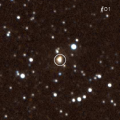
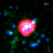
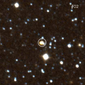
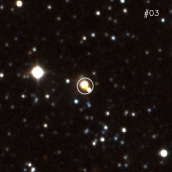
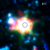
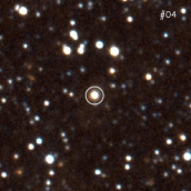
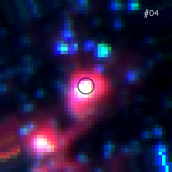
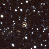
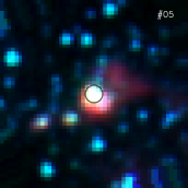
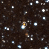
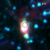
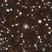
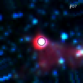
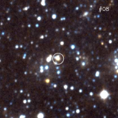
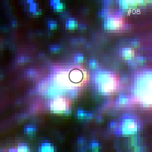
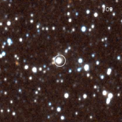
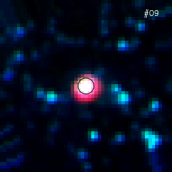
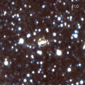
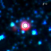
Figure 16: Colour-composite images for the YSO candidates in the SMC. For each object $J_{\rm s}K_{\rm s}$ (blue/ red) and Spitzer [3.6]-[5.8]-[8] images (blue/ green/ red) are shown. Each image is $1^{\prime}\times 1^{\prime}$ across and North is to the top and East to the left. For the last 2 objects we used IRSF images and show the $JHK$ colour-composite.

Appendix D Optical spectra

In this appendix we show all the optical spectra obtained as possible counterparts of the 34 IR sources in the SMC. As described in Section 3.5.1, the observed optical source is not always the correct counterpart for the IR source. No optical counterparts were found for sources #05, 06, 24, 29 and 31. The spectra form the basis of our optical classification scheme, using several emission lines. The last panel of Fig. 4 shows the identifications of the lines discussed in this work for source #26.

Figure 4: Optical spectra of possible optical counterparts for the IR sources in the SMC. No spectra were obtained for sources #24 and 31, and for sources #05, 06 and 29 the optical spectra are not associated with the IR sources. The most conspicuous spectral features are labelled in the last panel for source #26.

Figure 5: continued

Figure 6: continued

Figure 7: continued

Figure 8: continued

Figure 9: continued

The most conspicuous spectral features are labelled for source #26.

References

- André & Montmerle (1994) André P., Montmerle T., 1994, ApJ, 420, 837
- Angeloni et al. (2007) Angeloni R., Contini M., Ciroi S., Rafanelli P., 2007, AJ, 134, 205
- Banerji et al. (2009) Banerji M., Viti S., Williams D.A., Rawlings J.M.C., 2009, ApJ, 692, 283
- Barsony et al. (2010) Barsony M., Wolf-Chase G.A., Ciardi D.R., O’Linger J., 2010, ApJ, 720, 64
- Belczyński et al. (2000) Belczyński K., Mikołajewska J., Munari U., Ivison R.J., Friedjung M., 2000, A&AS, 146, 407
- Bernard-Salas & Tielens (2005) Bernard-Salas J., Tielens A.G.G.M., 2005, A&A, 431, 523
- Bolatto et al. (2007) Bolatto A.D. et al., 2007, ApJ, 655, 212
- Boogert et al. (2008) Boogert A.C.A. et al., 2008, ApJ, 678, 985
- Boyer et al. (2011) Boyer M.L. et al., 2011, AJ, 142, 103
- Corradi et al. (2010) Corradi R.L.M. et al., 2010, A&A, 509, 41
- Crawford et al. (2011) Crawford E.J., Filipović M.D., de Horta A.Y., Wong G.F., Tothill N.F.H., Drasković D., Collier J.D., Galvin T.J., 2011, SerAJ, 183, 95
- Draine (2011) Draine B.T., 2011, “Physics of the Interstellar and Intergalactic Medium”, Princeton University Press
- Draine & Li (2001) Draine B.T., Li A., 2001, ApJ, 551, 807
- Eisenhardt et al. (2004) Eisenhardt P.R., Stern D., Brodwin M., 2004, ApJS, 154, 48
- Fazio et al. (2004) Fazio G.G. et al., 2004, ApJS, 154, 10
- Filipović et al. (1998) Filipović M.D., Haynes R.F., White G.L., Jones P.A., 1998, A&AS, 130, 421
- Forbrich et al. (2010) Forbrich J. et al., 2010, ApJ, 716, 1453
- Furlan et al. (2006) Furlan E. et al., 2006, ApJS, 165, 568
- Furlan et al. (2008) Furlan E. et al., 2008, ApJS, 176, 184
- Galliano et al. (2008) Galliano F., Madden S.C., Tielens A.G.G.M., Peeters E., Jones A.P., 2008, ApJ, 679, 310
- Gerakines et al. (1995) Gerakines P.A., Schutte W.A., Greenberg J.M., van Dishoeck E.F., 1995, A&A, 296, 810
- Gerakines et al. (1999) Gerakines P.A. et al., 1999, ApJ, 522, 357
- Gibb et al. (2004) Gibb, E.L., Whittet D.C.B., Boogert A.C.A., Tielens A.G.G.M., 2004, ApJS, 151, 35
- Gordon et al. (2011a) Gordon K. et al., 2011a, AJ, 142, 102
-
Gordon et al. (2011b)
Gordon K. et al., 2011b, http://data.spitzer.caltech.edu/popular/
sage-smc/20110429_enhanced/documentation/sage-smc_delivery_apr11.pdf - Gruendl & Chu (2009) Gruendl R.A., Chu Y.-H., 2009, ApJS, 184, 172
- Habart et al. (2005) Habart E., Walmsley M., Verstraete L., Cazaux S., Maiolino R., Cox P., Boulanger F., Pineau des For ts G., 2005, SSRv, 119, 71
- Haynes et al. (2010) Haynes K., Cannon J.M., Skillman E.D., Jackson D.C., Gehrz R., 2010, ApJ, 724, 215
- Hoare et al. (2007) Hoare M.G., Kurtz S.E., Lizano S., Keto E., Hofner P., 2007, in “Protostars and Planets” V, eds. B. Reipurth, D. Jewitt, K. Keil, University of Arizona Press, Tucson, p. 181
- Houck et al. (2004) Houck J.R. et al., 2004, ApJS, 154, 18
- Jørgensen et al. (2006) Jørgensen J.K. et al., 2006, ApJ, 645, 1246
- Kato et al. (2007) Kato D. et al., 2007, PASJ, 59, 615
- Keller et al. (2008) Keller L.D. et al., 2008, ApJ, 684, 411
- Kemper et al. (2010) Kemper F. et al., 2010, PASP, 122, 683
- Kessler-Silacci et al. (2006) Kessler-Silacci J. et al., 2006, ApJ, 639, 275
- Lada (1987) Lada C.J., 1987, “Star Forming Regions”, eds. Peimbert M., Jugaku J., Proc. IAU Symp. 115, Dreidel, Dordrecht , p. 1
- Lahuis et al. (2010) Lahuis F., van Dishoeck E.F., Jørgensen J.K., Blake G.A., Evans N.J., 2010, A&A, 519, 3
- Lebouteiller et al. (2010) Lebouteiller V., Bernard-Salas J., Sloan G.C., Barry D.J., 2010, PASP, 122, 231
- Lee et al. (2006) Lee J.-E. et al., 2006, ApJ, 648, 491
- Ngeow & Kanbur (2008) Ngeow C., Kanbur S.M., 2008, ApJ, 679, 76
- Martayan et al. (2007) Martayan C., Floquet M., Hubert A.M., Gutierrez-Soto J., Fabregat J., Neiner C., Mekkas M., 2007, A&A, 472, 577
- Meixner et al. (2006) Meixner M. et al. 2006, AJ 132, 2268
- Mikołajewska (2004) Mikołajewska J., 2004, RMxAC, 20, 33
- Muench et al. (2007) Muench A.A., Lada C.J., Luhman K.L., Muzerolle J., Young E., 2007, AJ, 134, 411
- Oliveira et al. (2009) Oliveira J.M. et al., 2009, ApJ, 707, 1269
- Oliveira et al. (2011) Oliveira J.M. et al., 2011, MNRAS, 411, L36
- Parmar et al. (1991) Parmar P.S., Lacy J.H., Achtermann J.M., 1991, ApJ, 372, 25
- Pontoppidan et al. (2008) Pontoppidan K.M. et al., 2008, ApJ, 678, 1005
- Rho et al. (2006) Rho J., Reach W.T., Lefloch B., Fazio G.G., 2006, ApJ, 643, 965
- Rieke et al. (2004) Rieke G.H. et al., 2004, ApJS, 154, 25
- Robinson et al. (2012) Robinson G., Smith R.G., Maldoni M.M., 2012, MNRAS, 424, 1530
- Robitaille et al. (2007) Robitaille T.P., Whitney B.A., Indebetouw R., Wood K., 2007, ApJS, 169, 328
- Robitaille et al. (2006) Robitaille T.P., Whitney B.A., Indebetouw R., Wood K., Denzmore P., 2006, ApJS, 167, 256
- Rodgers et al. (1988) Rodgers A.W., Conroy P., Bloxham G., 1988, PASP, 100, 626
- Russell & Dopita (1992) Russell S.C., Dopita M.A., 1992, ApJ, 384, 508
- Sandstrom et al. (2012) Sandstrom K.M. et al., 2012, ApJ, 744, 20
- Sargent et al. (2009) Sargent B.A. et al., 2009, ApJS, 182, 477
- Schmid (1989) Schmid H.M., 1989, A&A, 211, 31
- Seale et al. (2009) Seale J.P., Looney L.W., Chu Y.-H., Gruendl R.A., Brandl B., Chen R.C.-H., Brandner W., Blake G.A., 2009, ApJ, 699, 150
- Seale et al. (2011) Seale J.P., Looney L.W., Chen C.-H.R., Chu Y.-H., Gruendl R.A., 2011, ApJ, 727, 36
- Shimonishi et al. (2010) Shimonishi T., Onaka T., Kato D., Sakon I., Ita Y., Kawamura A., Kaneda H., 2010, A&A 514, 12
- Smith et al. (2007) Smith J.D.T. et al., 2007, ApJ, 656, 770
- Spoon et al. (2002) Spoon H.W.W., Keane J.V., Tielens A.G.G.M., Lutz D., Moorwood A.F.M., Laurent O., 2002, A&A 385, 1022
- Sternberg & Neufeld (1999) Sternberg A., Neufeld D.A., 1999, ApJ, 516, 371
- Stetson (1987) Stetson P.B., 1987, PASP, 99, 191
- Störzer & Hollenbach (2000) Störzer H., Hollenbach D., 2000, ApJ, 539, 751
- Szewczyk et al. (2009) Szewczyk O., Pietrzyński G., Gieren W., Ciechanowska A., Bresolin F., Kudritzki R.-P., 2009, AJ, 138, 1661
- Torres et al. (2012) Torres A.F., Kraus M., Cidale L.S., Barbá R., Borges Fernandes M., Brandi E., 2012, MNRAS in press, arXiv:1209.2397
- van den Ancker (1999) van den Ancker M.E., 1999, PhD Thesis, University of Amsterdam
- (70) van den Ancker M.E., Tielens A.G.G.M., Wesselius P.R., 2000, A&A, 358, 1035
- van Dishoeck (2004) van Dishoeck E.F., 2004, ARA&A, 42, 119
- van Loon et al. (2005) van Loon J.Th. et al., 2005, MNRAS, 364, 71
- van Loon et al. (2008) van Loon J.Th. et al., 2008, AJ, 487, 1055
- van Loon et al. (2010a) van Loon J.Th. et al., 2010a, AJ, 139, 68
- van Loon et al. (2010b) van Loon J.Th., Oliveira, J.M., Gordon K.D., Sloan G.C., Engelbracht C.W., 2010b, AJ, 139, 68
- Werner et al. (2004) Werner M.W. et al., 2004, ApJS, 154, 1
- White & Hillenbrand (2004) White R.J., Hillenbrand L.A., 2004, ApJ, 616, 998
- Whitney et al. (2008) Whitney B.A. et al., 2008, AJ, 136, 18
- Wong et al. (2011a) Wong G.F., Filipović M.D., Crawford E.J., de Horta A.Y., Galvin T., Drasković D., Payne J.L., 2011a, SerAJ, 182, 43
- Wong et al. (2011b) Wong G.F. et al. 2011b, SerAJ, 183, 103
- Wong et al. (2012) Wong G.F. et al., 2012, SerAJ, 184, 93
- Woods et al. (2011) Woods Paul M. et al., 2011, MNRAS, 411, 1597
- Zasowski et al. (2009) Zasowski G., Kemper F., Watson D.M., Furlan E., Bohac C.J., Hull C., Green J.D., 2009, ApJ, 694, 459