Accurate Lower Bounds on Two-Dimensional Constraint Capacities From Corner Transfer Matrices

Abstract

We analyse the capacity of several two-dimensional constraint families — the exclusion, colouring, parity and charge model families. Using Baxter’s corner transfer matrix formalism combined with the corner transfer matrix renormalisation group method of Nishino and Okunishi, we calculate very tight lower bounds and estimates on the growth rates of these models. Our results strongly improve previous known lower bounds, and lead to the surprising conjecture that the capacity of the even and charge(3) constraints are identical.

I Introduction

In this paper, we analyse the capacity of several two-dimensional constraints. A constraint induces a model of magnetic spins, each of which can take a small number of spin values (typically 2, representing ‘up’ or ‘down’ magnetic spins). These spins are arranged in an ordered fashion on a two-dimensional plane — in all the models we analyse, they are positioned at the vertices of the square lattice $\mathbb{Z}^{2}$. Each constraint limits in some way the potential arrangements of the spins on the lattice.

An application where constraints arise is that of data storage. Here, the values of the spins contain data stored (in some encoding) on a magnetic disk. Due to properties of the disk, it may be undesirable for certain local arrangements of spins to exist, and this leads to a corresponding constraint. For example, in the hard squares model we define below, the spins can take the values $\oplus$ and $\ominus$. However, the presence of two $\ominus$ spins next to each other may cause magnetic interference, so we do not allow this to happen.

Given a constraint such as this, we wish to know what the storage capacity of the disk is. In the language of statistical mechanics, the partition function is the number of different configurations that can be written on $N$ spins under the constraint:

$$Z_{N}=(\mbox{\# of legal configurations on $N$ spins}).$$ (1)

We are interested in the behaviour of this number as the size of the storage array grows to infinity, and so define the partition function per site

$$\kappa=\lim_{N\rightarrow\infty}Z_{N}^{1/N}.$$ (2)

We also call $\kappa$ the growth rate of the model. The growth rate is directly related to the capacity of a constraint, which is defined to be the number of bits of information per spin that is possible to be written on a disk with that constraint:

$$\mbox{cap}(C)=\lim_{N\rightarrow\infty}\frac{1}{N}\log_{2}Z_{N}=\log_{2}\kappa.$$ (3)

In other words, a disk with $N$ spins can store approximately $\mbox{cap}(C)\times N$ bits of information under the constraint $C$. A ‘free’ disk with no constraints has a capacity of 1, since there are $2^{N}$ possible configurations on $N$ spins, and as such each spin represents one bit of information. As we approach this problem from a combinatorial point of view, we shall limit our terminology to growth rates rather than capacity (of course, they are trivial to derive from each other).

This problem is also studied in symbolic dynamics and dynamical systems, but with different terminology. Here, the capacity is also known as the (topological) entropy of the model, while the spins are letters (of an alphabet). Constraints are called sofic shifts (or systems), with a slight distinction: in constrained coding, the focus is on configurations of finite systems of arbitrary size, while in symbolic dynamics (and this paper), the focus is on configurations on the entire lattice. The exclusion and colouring models below are sub-classes of so-called ‘shifts of finite type’ or ‘finite memory systems’.

The capacity of constraints in one dimension is, in general, very easily computed using a transfer matrix. Unfortunately, capacities of two-dimensional constraints are significantly more difficult to compute, and because of this we seek estimates and rigorous lower and upper bounds for their values. Of interest here are the methods of Engel [1], and Calkin and Wilf [2], who provide a method to calculate such bounds using transfer matrices, illustrating with the hard squares model. Louidor and Marcus [3] generalised this method and applied it to the exclusion, parity and charge families of constraints discussed here. Additional references are provided for individual models as we introduce them below.

In this paper, we use corner transfer matrix (CTM) formalism to derive very precise lower bounds on the growth rates of the models that we study. The corner transfer matrix method was first devised by Baxter in 1968 [4] as a way of numerically estimating the growth rate of fully-packed dimers on a rectangular lattice. In later studies in the late 70s [5, 6], it was developed into method to calculate series expansions of the partition function and magnetisation. A particularly noteworthy triumph of this method was Baxter’s famous solution of the hard hexagons model [7, 8], which was derived by noticing a pattern in the eigenvalues of the corner transfer matrices.

As far as we know, CTM formalism has never been used before to calculate lower bounds, rather than estimates (although in fact, the theoretical machinery required to produce lower bounds has long been in place). When used for this purpose, the accuracy of the bound depends on how close we can come to the solution of the model.

For this purpose, we use the corner transfer matrix renormalisation group (CTMRG) method of Nishino and Okunishi [9, 10]. This method combines the original CTM method with ideas from the density matrix renormalisation group method (see, for example, [11, 12]), and also produces estimates of the growth rate. The CTMRG is more general and easier to apply numerically than Baxter’s original method, and has been applied, among other things, to self-avoiding walks [13] and the Ising model scaling function [14]. Recently, it too has been extended by one of the authors [15] to calculate series expansions.

In Section II, we define the models that we study and discuss some reformulations needed to make them amenable to CTM analysis. In Section III, we explain the corner transfer matrix formalism that we use to derive our lower bounds and estimates. These numerical results are presented in Section IV. In Section V, we discuss the (conjectured) equivalency between two of our models, and conclude in Section VI.

II The models

We calculate the growth rate of several models in this paper. All of these models have spins which lie on the vertices of a square lattice, which usually take the values $\oplus$ and $\ominus$. The configurations will be constrained in certain ways that we describe below.

II-A Exclusion models

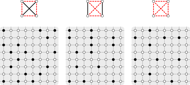
Figure 1: (bottom) Examples of the three exclusion models we consider (from left to right): hard squares, RWIM and NAK. We represent $\ominus$ spins by black vertices and $\oplus$ spins by white vertices. (top) The diagrams show the allowed configurations around a face for each model; two vertices joined by a solid line may be simultaneously occupied by $\ominus$s, while vertices joined by a dashed line may not.

In the exclusion models, we consider configurations of $\oplus,\ominus$ spins which are forbidden to contain certain local configurations of $\ominus$s (see Fig. 1).

Definition 1.

Consider a configuration of $\oplus,\ominus$ spins on the vertices of the square lattice.

• The configuration satisfies the hard squares constraint if it does not contain two $\ominus$ spins joined by a single bond. If one considers the $\ominus$ spins to be the centres of rotated square blocks, then this constraint requires that these blocks do not overlap.

  This model is a special case of a more general hard squares model where the constraint is enforced, but each $\ominus$ spin is also given a weight $z$. Our model corresponds to $z=1$. In the more general model, questions of interest include not only this special case, but also the location of the phase transitions (singularities in the free energy). These questions have been studied using corner transfer matrices in [6, 15]. Placing the spins on the vertices of a triangular lattice results in the hard hexagon model, which has been exactly solved using corner transfer matrices [7, 8]. Studies on the $z=1$ case include [2, 16].

• The configuration satisfies the read-write isolated memory (RWIM) constraint [17, 18] if it does not contain two $\ominus$ spins joined by a horizontal bond, or lying diagonally across a single face. This constraint can be used to model one-dimensional memory states with the hard square constraint, which are sequentially updated in such a way that no two adjacent spins are changed in the same update.

• The configuration satisfies the non-attacking kings (NAK) constraint if it does not contain two $\ominus$ spins joined by a single bond, or lying diagonally across a single face. Equivalently every face of the lattice contains at most one $\ominus$ spin. If one considers each $\ominus$ spin to be a king on a chessboard, then the NAK constraint requires that no king can attack another. This has been studied, along with the hard squares and other models, in [19].

II-B Colouring models

We also consider vertex colourings of the lattice; each vertex is coloured using labels from 0 to $q-1$ for some fixed $q$, and again we prohibit certain local configurations.

Definition 2.

A configuration of $\{0,\ldots,q-1\}$ spins satisfies the $q$-colouring constraint if it does not contain two nearest-neighbour spins with the same colour.

This is related to the chromatic polynomial and the anti-ferromagnetic Potts model (see for example [20, 21, 22, 23]). When $q=2$, there are only two possible configurations, while for $q=3$ it is known that the growth rate is exactly $(4/3)^{3/2}=1.539\,600\,7178\dots$ [24]. We study this model for higher $q$, where the growth rate is not known exactly.

II-C Parity models

Again we place the spins $\oplus$ and $\ominus$ at the vertices of the square grid. However unlike the models above, the constraints are no longer local. The two parity models arise by constraining the parity of the number of $\oplus$ spins lying between two $\ominus$ spins along any horizontal or vertical line.

Definition 3.

Consider a configuration of $\oplus,\ominus$ spins on the vertices of the square grid. Take any two $\ominus$ spins lying along a horizontal or vertical line so that there is no other $\ominus$ spin between them.

• If every such pair is separated by an even number of $\oplus$ spins, then the configuration satisfies the even constraint.

• Conversely, if every such pair is separated by an odd number of $\oplus$ spins, then the configuration satisfies the odd constraint.

While the above spin constraints are not local, it is possible to map them to other models of states with local constraints, which makes them amenable to CTM analysis. We explain this mapping below.

The growth rate of the odd model is known to be $\sqrt{2}$ [3]. To prove that the growth rate is at least $\sqrt{2}$, populate the lattice with $\oplus$ in a checkerboard pattern. The remaining spins, which constitute half the total spins, can then be assigned $\oplus$ or $\ominus$ independently. This always produces a valid configuration, so the bound follows.

To obtain the opposite bound, consider configurations of spins which obey the odd constraint along horizontal lines, while having no constraint along vertical lines. Being less constrained, the growth rate of this new model is greater than that of the odd model and is equal to the growth rate of the odd model in 1 dimension. It is straightforward to show that this is exactly $\sqrt{2}$.

Since the growth rate of the odd model is known exactly, we do not discuss it further.

II-D Charge(3) model

A final family of constraints is parameterised by a positive integer corresponding to the maximum cumulative electric ‘charge’ along a horizontal or vertical line. As we scan along a row or column, our cumulative ‘charge’ will increase by $+1$ or $-1$ each time we pass a $\oplus$ or $\ominus$ (respectively). We arrive at the charge model by constraining the allowed values of this cumulative charge.

Definition 4.

A configuration of $\oplus,\ominus$ spins satisfies the charge(3) constraint if for any finite horizontal or vertical line segment, the sum of the spins along that segment lies between $-3$ and $+3$.

Equivalently, starting from any given horizontal (resp. vertical) bond, there exists an initial charge between 0 and 3, so that scanning to the east (resp. south), the cumulative charge always lies between $0$ and $3$.

Clearly the above definition can be generalised by replacing $3$ by any other positive integer. There are only 2 valid charge(1) configurations — checkerboard patterns of $\oplus$ and $\ominus$ — so this system has growth rate 1. The growth rate of charge(2) configurations on $\mathbb{Z}^{d}$ was proved in [3] to be $2^{2^{-d}}$. Charge(3) is the first of this family of models for which the growth rate is unknown — indeed, previous works have been unable to determine its first digit exactly. Our results strongly support the following surprising conjecture:

Conjecture 1.

The charge(3) and even models have equal growth rate on $\mathbb{Z}^{2}$.

II-E Model transformations: states on bonds

The exclusion and colouring models all share the property that their constraint is local, acting entirely within the confines of a single cell. This is precisely what we need for the model to be amenable to analysis using corner transfer matrices. As such, we can apply this analysis to these models directly.

However, the even and charge(3) constraints are non-local. Fortunately, we can transform these models so that the constraints can be expressed in a local manner. To do this, we will map configurations of $\oplus$ and $\ominus$ spins on the vertices of the lattice to configurations of states that lie on the bonds of the lattice.

We first explain this process for the charge(3) model (as it is conceptually simpler). Here, the state of any horizontal (resp. vertical) bond is the cumulative charge on that bond, having read the spin to its west (resp. north). So in any valid configuration, all bonds will have integer states between 0 and 3 (inclusive). Considering the states around a vertex spin, the states of the south and east bonds must be 1 more or 1 less than those of the north and west bonds respectively (and the differences must be consistent with each other). That is,

$$\begin{array}[]{ccc}&a&\\ b\!\!&\circledast&\!\!c\\ &d&\end{array} =\begin{cases}\text{valid }&\text{ if }d-a=c-b=\pm 1\\ \text{invalid }&\text{ otherwise. }\end{cases}$$ (7)

We call this bond model the $Q$-charge model ($Q$ being traditional notation for charge in electrostatics).

Note that this mapping is not a bijection; it is possible for a single charge(3) configuration to correspond to many $Q$-charge configurations. If the cumulative charges along a given row take 4 different values, then only a single $Q$-charge configuration is possible on that row. However if the cumulative charges take only 2 or 3 values, then it is possible to increase or decrease those values and so create several possible $Q$-charge configurations along the row. However, these possibilities are not sufficient to change the growth rate of the model.

Lemma 2.

The growth rate of the charge(3) and $Q$-charge models are equal.

Proof:

The mapping defined above is one-to-many and so shows that $\kappa_{charge(3)}\leq\kappa_{\text{$Q$-charge}}$. To prove the reverse inequality, consider both constraints on the lattice $[1,N]^{2}$ (including boundary bonds).

Starting with a valid charge(3) configuration, the state of the first bond in each row/column may have up to 4 possible values (in fact, one of these values is always impossible, but this does not have an effect on the proof). After this, the row/column is fully determined. So on this finite lattice, every charge(3) configuration corresponds to at most $4^{2N}$ $Q$-charge configurations. Since there are $N^{2}$ vertices in this lattice, the growth rates are equal in the $N\to\infty$ limit. ∎

Now we apply a similar conversion to the even model. Here, the state of a given horizontal (resp. vertical) bond records the number of $\oplus$ spins lying between that bond and the first $\ominus$ to its west (resp. north). However, we do not need to know the total number of $\oplus$ passed, but only whether it is an even or odd number. Hence the states of each bonds will be ‘$p$’ or ‘$i$’ taken from the French pair and impair for even and odd. We chose this convention to avoid confusion between the names of these bond states and the names of the even and odd models.

All bonds adjacent to $\ominus$ spins are labelled ‘$p$’. Around any $\oplus$ spin, bonds on opposite sides of the vertex must take different labels — so a bond with a ‘$p$’ state must lie opposite a bond with an ‘$i$’ state and vice versa. This means that for any given $\ominus$ spin, if we scan east to the next $\ominus$ spin, we will pass an even number of $\oplus$ spins and so read an odd-length alternating sequence of bond states $pipi\dots ip$.

We call this new model the ‘$p$-$i$’ model. A labelling of bonds by $p$ and $i$ will be valid for this model when there are no two adjacent $i$ states along any horizontal or vertical line, and any vertex must be adjacent to zero or two $i$ states.

Again, this mapping is not bijective, as there are two possible $p$-$i$ configurations for a row which contains only $\oplus$ spins in the even model, namely $pipi\dots$ or $ipip\dots$. However, it is again easy to show that the growth rate is unchanged.

Lemma 3.

The growth rate of the even model is equal to that of the $p$-$i$ model.

Proof:

The proof is identical to that of the previous lemma, except that there are at most two possible ways to determine each row or column. This means that every even configuration corresponds to at most $2^{2N}$ $p$-$i$ configurations, which is still sub-exponential in the number of vertices in the lattice (which is $N^{2}$). ∎

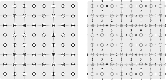
Figure 2: An example of a valid charge(3) configuration (left) and one of the $Q$-charge configurations that it maps to (right).

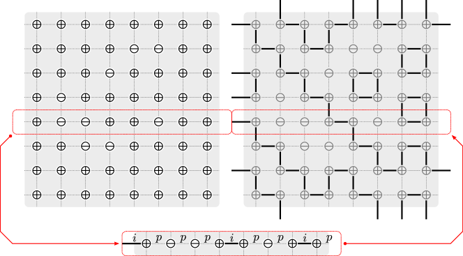
Figure 3: An example of a valid even configuration (left) and one of the $p$-$i$ configurations it maps to (right). In the under-set figure we show explicitly how one row of the even configuration is mapped to a row in the $p$-$i$ model. Bonds between $\ominus$ spins are labelled by an odd length sequence $pipi\dots\ p$. To visualise this we occupy each bond labelled by $i$. Notice that each vertex has degree 0 or 2, and that if two occupied bonds meet at a vertex, then they must be orthogonal to each other.

II-F Model transformations: states on faces

We make a further transformation from the $p$-$i$ model to another model (which we call even-face), which places states on the centres of the faces of the lattice. These states can take the values 0 or 1. It is not necessary to make this transformation, but empirically it responds better to the corner transfer matrix renormalisation group method.

Consider each bond in state ‘$i$’ in a $p$-$i$ configuration to be occupied (see Fig. 3). Each vertex in a valid configuration is incident to either 0 or 2 occupied bonds, and these form distinct simple loops which separate the plane into regions. We now properly colour these regions with 2 colours, and define the state of each face to be its colour.

Thus, given a $p$-$i$ configuration, two states on neighbouring faces in the corresponding even-face configuration are equal if they are separated by a $p$ bond (since they are part of the same region), and unequal otherwise (since they are separated by an occupied bond and so in different regions). A full enumeration of the possible $p$-$i$ configurations shows that the resulting configuration is internally consistent (see Fig. 4). Now we determine the validity of a configuration according to each cell:

$$\begin{pmatrix}a&b\\ c&d\end{pmatrix} =\begin{cases}\mbox{invalid}&\mbox{if $a+b+c+d=2$}\\ \mbox{valid}&\mbox{otherwise.}\end{cases}$$ (8)

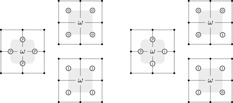
Figure 4: Possible cells in the $p$-$i$ and even-face models, up to rotation.

Again, this mapping is not a bijection, but determining the value of one state on an arbitrary face in the even-face model will fully determine the rest of the configuration. As such, the number of even-face configurations is exactly twice the number of $p$-$i$ configurations, and their growth rates are equal.

III Corner transfer matrix formalism

III-A Computing a rigorous lower bound

Consider, for the sake of exposition, a model in which spins lie on the vertices of $\mathbb{Z}^{2}$ and can take two values. Further, the model is governed by an ‘interaction round a face’ $\omega$ that is symmetric across a vertical line. This includes the exclusion models (hard squares, NAK and RWIM), the colouring models and the even-face model (since the square lattice is self-dual). More work is required for the charge model and we discuss it further below. We wish to count the number of configurations, and so take

$$\omega\!\begin{pmatrix}a&b\\ c&d\end{pmatrix} =\begin{cases}1&\text{if the local configuration is valid}\\ 0&\text{otherwise.}\end{cases}$$ (9)

First consider a strip of the square lattice of height $m$ with cylindrical boundary conditions identifying the top and bottom edges. Let $V$ be the $2^{m}\times 2^{m}$ column transfer matrix defined by

$$V_{\sigma,\tau} =\prod_{i=1}^{m}\omega\!\begin{pmatrix}\sigma_{i+1}&\tau_{i+1}\\ \sigma_{i}&\tau_{i}\\ \end{pmatrix}$$ (10)

where $\sigma_{m+1}\equiv\sigma_{1}$ and similarly for $\tau$. See Fig. 5. Note that this is just the traditional column transfer matrix and is symmetric.

Since $V$ is symmetric, we can apply a variational principle — namely, the dominant eigenvalue $\Lambda(m)$ is given by

$$\Lambda(m) =\max_{\psi}\frac{\psi^{T}V\psi}{\psi^{T}\psi}.$$ (11)

The growth rate of the system is the limit

$$\kappa =\lim_{m\to\infty}\Lambda(m)^{1/m}.$$ (12)

To obtain a lower bound, it suffices to substitute a particular $\psi$ into (11), which we do using Baxter’s corner transfer matrix ansatz.

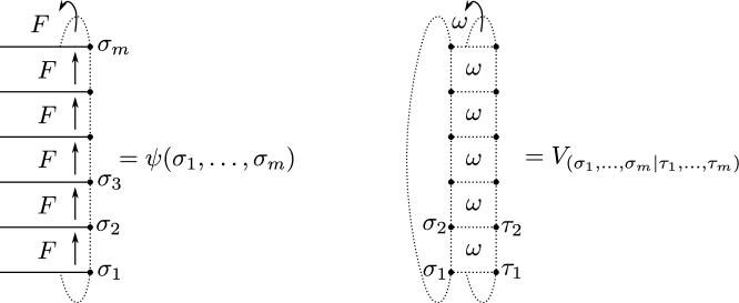
Figure 5: We define the $2^{m}$ elements of the vector $\psi$ to be the trace of the product of $F$ matrices. The elements of the column transfer matrix $V$ are products of the face weight $\omega$. In both cases we apply cylindrical boundary conditions so that $\sigma_{m+1}\equiv\sigma_{1}$ and $\tau_{m+1}\equiv\tau_{1}$.

Let $\left\{F(a,b)\right\}$ be a set of four $n\times n$ matrices indexed by two spin values $a,b\in\left\{0,1\right\}$ so that $F(a,b)=F^{T}(b,a)$. While some of these matrices may be zero (e.g. for the hard squares model $F(1,1)=\mathbf{0}$), they should not all be trivial. Consider the vector of dimension $2^{m}$ which satisfies

$$\psi_{\sigma} =\operatorname{Tr}\left[F(\sigma_{1},\sigma_{2})F(\sigma_{2},\sigma_{3})\dots F(\sigma_{m},\sigma_{1})\right].$$ (13)

This is shown in Fig. 5. For any particular choice of $F$, we obtain a vector $\psi$ and so a lower bound for the maximisation problem. Now, given a choice of $F$, we need to be able to compute $\psi^{T}V\psi$ and $\psi^{T}\psi$ and so our lower bound.

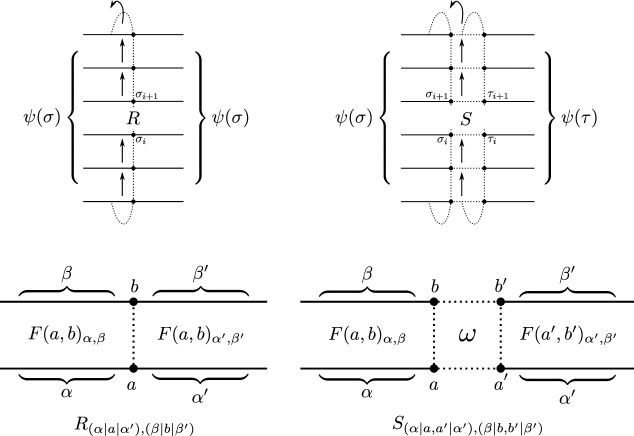
Figure 6: In order to compute $\psi^{T}\psi$ (top-left) and $\psi^{T}V\psi$ (top-right), we define two matrices $R$ and $S$ so that $\psi^{T}\psi=\operatorname{Tr}(R^{m})$ and $\psi^{T}V\psi=\operatorname{Tr}(S^{m})$. The elements of $R$ and $S$ are defined as indicated (bottom-left and bottom-right respectively).

Let us fix $m$ and the matrices $F$. We denote the $n^{2}$ entries of $F(a,b)$ as $F(a,b)_{\alpha,\beta}$ for $\alpha,\beta\in\left\{1,\dots,n\right\}$. It is possible to rewrite the product of $\psi^{T}\psi$ as the trace of a power of a new matrix, $R$. This is extremely helpful because $R$ is not dependent on the height of the strip. Instead, the height dependence is confined to the power of the matrix. In particular, we may write

$$\psi^{T}\psi =\operatorname{Tr}(R^{m})$$ (14)

where $R$ is a $(2n^{2})\times(2n^{2})$ matrix defined by

$$R_{(\alpha|a|\alpha^{\prime}),(\beta|b|\beta^{\prime})} =F(a,b)_{\alpha,\beta}F(a,b)_{\alpha^{\prime},\beta^{\prime}}.$$ (15)

See Fig. 6 for an illustration of this. To see this consider

$$\psi^{T}\psi =\sum_{\sigma}\left(\operatorname{Tr}\prod_{i=1}^{m}F(\sigma_{i},\sigma_{i+1})\right)^{2}$$ (16a)

$$=\sum_{\sigma}\left(\sum_{\alpha_{1},\dots,\alpha_{m}}\prod_{i=1}^{m}F(\sigma_{i},\sigma_{i+1})_{\alpha_{i},\alpha_{i+1}}\right)^{2}$$ (16b)

$$=\sum_{\sigma}\sum_{\alpha_{1},\dots,\alpha_{m}}\sum_{\alpha_{1}^{\prime},\dots,\alpha_{m}^{\prime}}\prod_{i=1}^{m}F(\sigma_{i},\sigma_{i+1})_{\alpha_{i},\alpha_{i+1}}F(\sigma_{i},\sigma_{i+1})_{\alpha_{i}^{\prime},\alpha_{i+1}^{\prime}}.$$ (16c)

Now rewrite the summands as elements of $$R$$

$$=\sum_{\sigma}\sum_{\alpha_{1},\dots,\alpha_{m}}\sum_{\alpha_{1}^{\prime},\dots,\alpha_{m}^{\prime}}\prod_{i=1}^{m}R_{(\alpha_{i}|\sigma_{i}|\alpha_{i}^{\prime}),(\alpha_{i+1}|\sigma_{i+1}|\alpha_{i+1}^{\prime})}$$ (16d)

$$=\operatorname{Tr}(R^{m}).$$ (16e)

In a similar way,

$$\psi^{T}V\psi =\operatorname{Tr}(S^{m})$$ (17)

where $S$ is a $(4n^{2})\times(4n^{2})$ matrix defined by

$$S_{(\alpha|a,a^{\prime}|\alpha^{\prime}),(\beta|b,b^{\prime}|\beta^{\prime})} =F(a,b)_{\alpha,\beta}\cdot\omega\begin{pmatrix}b&b^{\prime}\\ a&a^{\prime}\end{pmatrix}\cdot F(a^{\prime},b^{\prime})_{\alpha^{\prime},\beta^{\prime}}.$$ (18)

Note that due to the symmetry $F(a,b)=F^{T}(b,a)$, both $R$ and $S$ are symmetric.

Now let $\xi$ and $\eta$ be the maximal eigenvalues of $R$ and $S$ respectively. Our lower bound becomes

$$\Lambda(m) \geq\frac{\operatorname{Tr}(S^{m})}{\operatorname{Tr}(R^{m})} \Rightarrow\kappa =\lim_{m\to\infty}\Lambda(m)^{1/m}\geq\frac{\eta}{\xi}.$$ (19)

So to compute our bound it suffices to compute the dominant eigenvalues of $R$ and $S$.

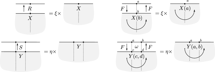
Figure 7: (left) $X$ and $Y$ are the dominant eigenvectors of the matrices $R$ and $S$ (respectively) with eigenvalues $\xi$ and $\eta$ (respectively). (right) By recasting $X$ and $Y$ as matrices, we can rewrite the eigenvalue equations as matrix equations in terms of $F$ as shown.

Let $X$ be the dominant eigenvector of $R$, so that

$$\xi X =RX.$$ (20)

See Fig. 7. It is helpful in what follows to recast $X$ as a set of matrices, and the corresponding eigenvalue equation as a matrix equation. The vector $X$ has dimension $2n^{2}$ and we index its elements as $X_{(\alpha|a|\beta)}$. Define $X(a)_{\alpha,\beta}=X_{(\alpha|a|\beta)}$. Then we can write the eigenvalue equation as

$$\xi X(a)_{\alpha,\alpha^{\prime}} =(RX)_{(\alpha|a|\alpha^{\prime})}$$ (21a)

$$=\sum_{\beta,b,\beta^{\prime}}R_{(\alpha|a|\alpha^{\prime}),(\beta|b|\beta^{\prime})}X_{(\beta|b|\beta^{\prime})}$$ (21b)

$$=\sum_{\beta,b,\beta^{\prime}}F(a,b)_{\alpha,\beta}F(a,b)_{\alpha^{\prime},\beta^{\prime}}X(b)_{\beta,\beta^{\prime}}$$ (21c)

$$=\sum_{\beta,b,\beta^{\prime}}F(a,b)_{\alpha,\beta}\,X(b)_{\beta,\beta^{\prime}}\,F(b,a)_{\beta^{\prime},\alpha^{\prime}}$$ (21d)

$$=\left(\sum_{b}F(a,b)\,X(b)\,F(b,a)\right)_{\alpha,\alpha^{\prime}}$$ (21e)

and so

$$\xi X(a) =\sum_{b}F(a,b)\,X(b)\,F(b,a).$$ (22)

Now define $Y$ to be the dominant eigenvector of $S$, so $\eta Y=SY$. It is of dimension $4n^{2}$, and we index its elements as $Y_{(\alpha|a,b|\beta)}$. Again, partition these as $Y(a,b)_{\alpha,\beta}=Y_{(\alpha|a,b|\beta)}$. With similar working, we have the eigenvalue equation

$$\eta Y(a,b) =\sum_{c,d}\omega\begin{pmatrix}a&b\\ c&d\end{pmatrix}F(a,c)\,Y(c,d)\,F(d,b).$$ (23)

To compute $\xi$ and $\eta$, one could apply the power method to the matrices $R$ and $S$ using a random initial vector. However, since $R$ and $S$ have dimension $O(n^{2})$, each matrix-vector multiplication (and so each iteration) would take $O(n^{4})$ operations. Instead it is more efficient to apply the power method implicitly using (22) and (23).

Consider equation (22). Given a prospective eigenvector $X_{i}(a)$ with a fixed normalisation, we substitute this into the right-hand side of (22). Given this normalisation, the next iteration $\xi_{i+1},X_{i+1}(a)$ is now given by the left-hand side of the equation. Each iteration of these equations involves multiplying square matrices of dimension $n$, and so requires $O(n^{3})$ operations (or smaller with the use of more sophisticated algorithms).

We can use any value of $X(a)$ to start the power method, but the CTMRG method below will suggest an appropriate starting value. To cover the possibility that this starting value is a sub-dominant eigenvector, we perturb it slightly before starting the power method. $\eta$ (and $Y$) is found in an identical manner, except this perturbation is not needed (the result will still give a lower bound on $\eta$ and so $\kappa$).

So our process for computing a rigorous lower bound for $\kappa$ is this: we take any set of $F$ matrices, apply the power method to (22) and (23) to calculate $\eta$ and $\xi$, and then our lower bound is $\eta/\xi$.

Of course, the efficacy of this approach depends critically on the set of $F$ matrices — thus we now need a heuristic to find a ‘good’ set of $F$ matrices. This is achieved by use of the corner transfer matrix renormalisation group algorithm, which we detail in the next section.

We note that the method described in Sections 3 and 6 of [3] is similar in spirit to that described above, in that they both replace the eigenvector of the transfer matrix with an expression that simplifies calculations.

III-B Corner transfer matrix renormalisation group method

We now wish to choose a set of $F$ matrices which provide a good lower bound, i.e. as large as possible. We do this using a heuristic algorithm known as the corner transfer matrix renormalisation group (CTMRG) method. Note that while the choice of $F$ alters the quality of the bound, it does not affect the fact that it is a lower bound, and as such it is unnecessary to prove any convergence properties of the CTMRG method.

Since we wish our lower bound to be as large as possible, we wish to maximise $\eta/\xi$ with respect to $F$. The derivation of equations which ensure this is long and complicated, and we shall not repeat it here. It is sufficient [5] to note that if we have a set of $n\times n$ matrices $A(a)$ which satisfy

$$X(a) =A^{2}(a) Y(a,b) =A(a)\,F(a,b)\,A(b)$$ (24)

then $\kappa$ is stationary with respect to $F$. Note that defining $A$ in this way assumes that the model is invariant under rotation by $\pi/2$. For models without this symmetry, we define several different corner transfer matrices — see the next section. Unfortunately (24) does not prove that $\kappa$ is maximal, merely stationary, though empirically this does appear to be the case. See Fig. 8 for a graphical interpretation of the above equations. Unlike the more familiar column and row transfer matrices, the matrix $A(a)$ (the eponymous corner transfer matrix) adds the weight of one quadrant or corner of the lattice.

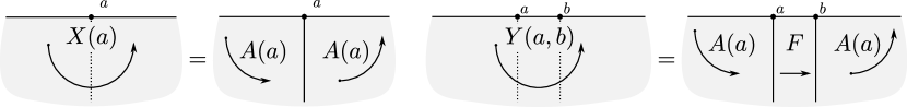
Figure 8: In Fig. 7 the eigenvectors $X$ and $Y$ were recast as matrices. Now we rewrite them again as products of the matrix $F$ together with the corner transfer matrix $A$. The matrix $F$ sweeps through a half-row or half-column and the matrix $A$ sweeps through a quarter of the lattice.

The CTMRG method calculates matrices which converge to the finite-size solution of (22), (23) and (24), known collectively as the CTM equations. As such, the $F$ matrices that it produces can be used in our calculations above to provide (what appears to be) a very tight lower bound.

To gain an intuition for the CTMRG method, consider $A(a)$ and $F(a,b)$ to be infinite-size transfer matrices (with an appropriate normalisation) which represent a corner and half-row of the entire plane respectively. It is easily seen that with $X$ and $Y$ determined according to (24), they represent (normalised) half-plane transfer matrices. In this case, (22) and (23) are seen to be satisfied by this choice of $F$, $X$ and $Y$. So the infinite-dimensional solution of the CTM equations can be thought of as a set of transfer matrices.

In order to approximate this infinite-dimensional solution, we can construct initial $A$ and $F$ matrices as the corner and half-row transfer matrices of a lattice of $(2p+1)\times(2p+1)$ spins. These matrices have dimension $2^{p}\times 2^{p}$. We can now bootstrap to a larger lattice by constructing the block matrices

$$A_{l}(c)|_{d,a} =\sum_{b}\omega\begin{pmatrix}a&b\\ c&d\end{pmatrix}F(d,b)\,A(b)\,F(b,a)$$ (25a)

$$F_{l}(d,c)|_{b,a} =\omega\begin{pmatrix}a&b\\ c&d\end{pmatrix}F(b,a)$$ (25b)

each having dimension $2^{p+1}\times 2^{p+1}$. From Fig. 9, it is apparent that $A_{l}$ and $F_{l}$ are the corner and half-row transfer matrices of a lattice of $(2p+3)\times(2p+3)$ spins. By repeating this process indefinitely, we approach the infinite-size transfer matrices which we require.

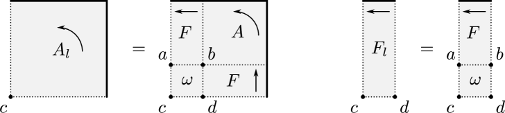
Figure 9: Expansion of transfer matrices.

At any $p$, we can compute the number of configurations on the lattice of size $(2p+1)\times(2p+1)$ as $Z_{2p+1,2p+1}=\sum_{a}\operatorname{Tr}\left(A^{4}(a)\right)$. Unfortunately, since the size of these matrices grows exponentially, this is not a practical approach for even moderate $p$. It does, however, suggest that we should examine the eigenvalues of $A$. If the eigenspectrum of $A$ decays quickly, then we can approximate this trace by using only the largest few eigenvalues of $A$.

To manipulate the eigenvalues directly, we diagonalise the matrix $A_{l}$. Observe that the CTM equations are invariant under the similarity transforms

$$A(a) \mapsto P^{T}(a)\,A(a)\,P(a) F(a,b) \mapsto P^{T}(a)\,F(a,b)\,P(b)$$ (26a)

$$X(a) \mapsto P^{T}(a)\,X(a)\,P(a) Y(a,b) \mapsto P^{T}(a)\,Y(a,b)\,P(b)$$ (26b)

for orthogonal matrices $P(a)$. This means that we can take $A_{l}(a)$ to be diagonal, with entries ordered from largest to smallest. We throw away the smaller eigenvalues by truncating our large matrices to size $n\times n$. Since the discarded eigenvalues are small, the effect of this truncation on the trace (and so our estimate of $Z_{2p+1,2p+1}$) will also be small. Empirically we also find that the resulting matrices are close to the $n\times n$ solution of the CTM equations.

Ideally, we would find approximate solutions at size $n\times n$ by using (25) to construct very large transfer matrices, then transform and truncate these transfer matrices according to (26). However, since the matrices double in size for each use of (25), this quickly becomes impractical.

Instead, we transform and truncate the matrices every time we expand. Since we may choose exactly how many eigenvalues to discard, we can take matrices of size $n\times n$, expand them to size $2n\times 2n$ and then truncate back down to size $n\times n$. In this way we can produce a sequence of $n\times n$ matrices which appear to converge to the finite-size solution of the CTM equations.

As far as we know, it is not proved that this procedure will converge at all, let alone to the finite-size solution. However, this happens empirically, and as stated above such a proof is not necessary to establish a rigorous lower bound — we can simply observe that the resulting $F$ matrices result in good bounds. In full, the CTMRG method is as follows:

1. Start with initial $1\times 1$ matrices $A(a),F(a,b)$ and let $n=1$.

2. Expand $A$ and $F$ using (25).

3. If required, increase $n$ by 1.

4. Diagonalise $A_{l}(a)$. Let $P(a)$ be the matrix consisting of the eigenvectors corresponding to the $n$ largest eigenvalues of $A(a)$.

5. Reduce $A_{l}$ and $F_{l}$ using (26).

6. Normalise $A$ and $F$ so that the top-left elements of $A(0)$ and $F(0,0)$ are both 1.

7. Go to step 2.

Once the above procedure has converged sufficiently at a given size $n$, we can substitute the resulting $F$ into the CTM equations to obtain $\xi$ and $\eta$ and the lower bound. In fact, we can terminate the procedure at any stage, since any $F$ will result in a bound, but in practice we wait until the procedure has converged to a desired precision.

We calculate our estimates of $\kappa$ by the formula [5]

$$\kappa =\frac{\left(\sum_{a}\operatorname{Tr}A^{4}(a)\right)\left(\sum_{a,b,c,d}\operatorname{Tr}\omega\begin{pmatrix}a&b\\ c&d\end{pmatrix}A(a)F(a,c)A(c)F(c,d)A(d)F(d,b)A(b)F(b,a)\right)}{\left(\sum_{a,b}\operatorname{Tr}A^{2}(a)F(a,b)A^{2}(b)F(b,a)\right)^{2}}.$$ (27)

Each term in this formula represents the partition function of the entire plane. However, the term in the denominator contains an extra row compared to the first term in the numerator, while the second term in the numerator contains both an extra row and column. The net effect is to cancel out everything but the effect of a single cell. In practice, using this formula is faster and more accurate than the lower bound computation, but of course does not provide a bound.

III-C Asymmetry and the CTMRG

The decomposition in (24), and thus the CTMRG, implicitly assumes that the corner transfer matrices are equal under a rotation of $\pi/2$. This naturally occurs if the model itself is invariant under this rotation, which holds true for the majority of the models we analyse. The exceptions are the RWIM and $Q$-charge models, which are only symmetric under rotation by $\pi$. To accommodate this, we define separate half-row and half-column transfer matrices, and two different families of corner transfer matrices — see Fig. 10.

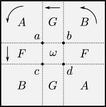
Figure 10: For a model with symmetry under rotation by $\pi$ we need two sets of corner transfer matrices $A$ and $B$ as well as half-row and half-column transfer matrices $F$ and $G$.

We will use $A$ to denote the corner transfer matrices for the second and fourth quadrants of the lattice, and $B$ for the first and third. Similarly we let $F$ and $G$ denote the half-row and half-column transfer matrices respectively. We expand these matrices in a similar way to (25), taking care with the orientations:

$$A_{l}(d)|_{b,c} =\sum_{a}\omega\begin{pmatrix}a&b\\ c&d\end{pmatrix}G(b,a)\,A(a)\,F(a,c) F_{l}(c,a)|_{d,b} =\omega\begin{pmatrix}a&b\\ c&d\end{pmatrix}F(d,b)$$ (28a)

$$B_{l}(c)|_{d,a} =\sum_{b}\omega\begin{pmatrix}a&b\\ c&d\end{pmatrix}F(d,b)\,B(b)\,G(b,a) G_{l}(d,c)|_{b,a} =\omega\begin{pmatrix}a&b\\ c&d\end{pmatrix}G(b,a).$$ (28b)

To reduce the matrices, we observe that we can represent the transfer matrix of the entire plane as either $(AB)^{2}$ or $(BA)^{2}$, and these are not necessarily equal. In order to diagonalise both these matrices and simultaneously preserve the CTM equations, we define $P_{AB}(a)$ and $P_{BA}(a)$ to be the matrices consisting of the first $n$ eigenvectors of $A_{l}(a)B_{l}(a)$ and $B_{l}(a)A_{l}(a)$ respectively. Our reducing transformations then become

$$A(a) \mapsto P_{AB}^{T}(a)\,A_{l}(a)\,P_{BA}(a) F(a,b) \mapsto P_{BA}^{T}(a)\,F_{l}(a,b)\,P_{BA}(b)$$ (29a)

$$B(a) \mapsto P_{BA}^{T}(a)\,B_{l}(a)\,P_{AB}(a) G(a,b) \mapsto P_{AB}^{T}(a)\,G_{l}(a,b)\,P_{AB}(b).$$ (29b)

The remainder of the method is unchanged.

III-D States on bonds

The CTMRG is defined on a model where the states are located on the vertices of the $\mathbb{Z}^{2}$ lattice. As this lattice is self-dual, it can be applied without change to a model where the states are on the faces. However, we must make some small adjustments when the states lie on the bonds, as for the $Q$-charge model. As this model is not invariant under a rotation of $\pi/2$, we will also use the machinery developed in the previous section.

In order to apply the CTMRG to this form of model, we use a form of the method similar to that developed by Foster and Pinettes [25, 13]. The face weight $\omega$ becomes a weight around a vertex, and we shift all the matrices by half a length unit (see Fig. 11). This also has the effect that the corner transfer matrices are no longer parameterised by a state — so we only have one $A$ and one $B$. Similarly the half-row and half-column matrices, $F(a)$ and $G(a)$, are now parameterised by a single state.

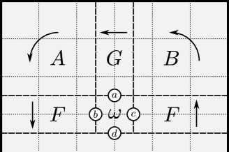
Figure 11: For a model with bond states we define the corner transfer matrices $A$ and $B$, and the half-row and half-column matrices $F$ and $G$ as shown. The edges of the lattice are shown in thin dotted lines. The bond-states surrounding the weight $\omega$ are shown as labelled white circles.

We make obvious adjustments to the expansion and contraction of the matrices. These now become

$$A_{l}|_{c,d} =\sum_{a,b}\omega\!\begin{pmatrix}&a&\\[-3.01385pt] b&&c\\[-3.01385pt] &d&\end{pmatrix}G(a)\,A\,F(b) F_{l}(b)|_{d,a} =\sum_{c}\omega\!\begin{pmatrix}&a&\\[-3.01385pt] b&&c\\[-3.01385pt] &d&\end{pmatrix}F(c)$$ (30a)

$$B_{l}|_{d,b} =\sum_{a,c}\omega\!\begin{pmatrix}&a&\\[-3.01385pt] b&&c\\[-3.01385pt] &d&\end{pmatrix}F(c)\,B\,G(a) G_{l}(d)|_{c,b} =\sum_{a}\omega\!\begin{pmatrix}&a&\\[-3.01385pt] b&&c\\[-3.01385pt] &d&\end{pmatrix}G(a)$$ (30b)

$$A \mapsto P_{AB}^{T}\,A_{l}\,P_{BA} F(a) \mapsto P_{BA}^{T}\,F_{l}(a)\,P_{BA}$$ (30c)

$$B \mapsto P_{BA}^{T}\,B_{l}\,P_{AB} G(a) \mapsto P_{AB}^{T}\,G_{l}(a)\,P_{AB}$$ (30d)

where the face weight $\omega$ is given by (7).

Note that the corner transfer matrix formalism which leads to the rigorous lower bound only requires that the original column transfer matrix $V$ is symmetric. In the case of the charge model, the symmetry of $V$ follows from the fact that if you invert all the vertex spins in a column, then the column is still legal. However, it is no longer the case that $F^{T}(a)=F(a)$ and our eigenvalue equations must be changed to reflect this:

$$\xi X =\sum_{a}F(a)\,X\,F^{T}(a)$$ (31a)

$$\eta Y(a) =\sum_{b,c,d}\omega\!\begin{pmatrix}&a&\\[-3.01385pt] b&&c\\[-3.01385pt] &d&\end{pmatrix}F(b)\,Y(d)\,F^{T}(c).$$ (31b)

In practice, applying the power method using these equations can be unstable for the $Q$-charge model for reasons we have not been able to determine. In any case, we are able to obtain significantly better bounds for this model through a relation to the even model (see Section V).

IV Results

The CTMRG algorithm described in the previous section was implemented in C++ using the Eigen numerical linear algebra library [26]. The main advantage of Eigen over other libraries is that it readily supports multiple precision computations through the MPFR library [27]. The eigenvalues of the corner transfer matrices range over many orders of magnitude, so all computations must be done at very high precision. For example, for the hard squares model, the eigenvalues of $A(0)$ and $A(1)$ at size $50\times 50$ range from $2^{0}$ down to approximately $2^{-50}$.

All of the computations were run on modest desktop computers running Linux and took between a few hours and a few days to complete. The fastest computation (overall) was hard squares and the slowest was charge(3). Indeed, our most precise results were for hard squares and the least precise were for charge(3).

Matrix diagonalisation requires $O(n^{3})$ operations, and so a full iteration of the algorithm described in Section III-B also requires $O(n^{3})$ operations. We have observed that for most of the models, the number of iterations required to converge at size $n$ does not increase with $n$. However, since our computer code waits until convergence at every size before proceeding, we observe that the algorithm is roughly $O(n^{4})$. Note however, that this is the time taken to converge at a fixed matrix size, not to a fixed number of digits in $\kappa$.

The rate of convergence of our estimates and bounds depends upon the eigenspectrum of the corner transfer matrices. For the purposes of this discussion we will assume that the matrices at each size have converged to their limiting value under the renormalisation procedure. A key observation is that the largest eigenvalues do not change much with matrix size — the 4 eigenvalues of $A(0)$ at size 4 are nearly the same as the 4 dominant eigenvalues of $A(0)$ at size 40, and presumably at size 400.

Thus, what changes as we increase matrix size are the eigenvalues we discard by truncating the matrices. Since each term in our computation of $\kappa$ (via (27)) is the trace of the product of 4 corner transfer matrices (some interlaced with half-row and half-column transfer matrices), we expect that the contribution of each eigenvalue to the estimate of $\kappa$ is roughly proportional to its fourth power.

The question of the tightness of the bound is a little more complicated, as it depends on how close our $F$ matrices are to the solution of the CTM equations. If they exactly solve the CTM equations at finite size (for some values of the other matrices), then there is no difference between our bound calculation using (19) and our estimate using (27), and so the error should be the same. As we run the algorithm to convergence at each finite size, we expect that the extra error induced by having a not-quite-optimal $F$ is minimal.

This analysis shows that the utility of the method hinges on the distribution of the eigenvalues of the corner transfer matrices. If the eigenvalues decay slowly, then by truncating the matrices we will throw away quite large contributions to the estimates and bounds of $\kappa$. In such a situation, we would expect our estimates and bounds to converge slowly with increasing matrix size. On the other hand, if the eigenvalues decay quickly then the truncated eigenvalues will have little impact.

It is believed [28] that the eigenvalues of the corner transfer matrices scale as

$$\lambda_{k}\sim\exp\left(-c(\ln k)^{2}\right).$$ (32)

Here we have denoted the $k^{\text{th}}$ largest eigenvalue by $\lambda_{k}$; since these do not vary significantly between different matrix sizes, we have not specified the dimension of the underlying matrix.

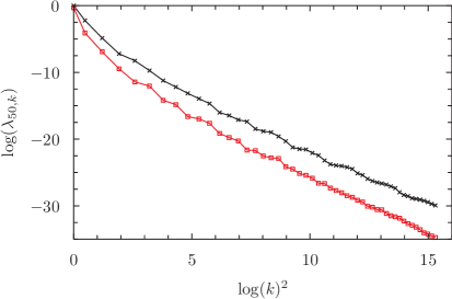
Figure 12: A plot of $\log(\lambda_{k})$ vs $\log(k)^{2}$, for the eigenvalues of $A(0)$ (upper curve) and $A(1)$ (lower curve) at size 50 for the hard squares model. For larger $k$, the plots appear approximately linear, supporting the conjectured scaling form of (32).

If the above scaling form holds true — and our observations suggest that it does (see Fig. 12) — then we expect the error in our estimates to have a similar asymptotic form with increasing matrix size. Thus, to achieve an error approximately $\varepsilon$, we need to take matrices of size $k\times k$ with

$$k \sim\exp\left(\alpha\sqrt{-\log(\varepsilon)}\right).$$ (33)

Substituting $\varepsilon=2^{-N}$ gives

$$k \sim\exp\left(\beta\sqrt{N}\right).$$ (34)

Since the running time and memory required grow polynomially with matrix size, the above argument supports the assertion that the time and memory required by the algorithm to correctly compute $N$ digits grows subexponentially with $N$.

TABLE I: Lower bounds and estimates for the growth rates of the various models. For each model we give the full decimal expansion of the lower bound, and then we give the last few digits of our estimate in brackets. These replace that many digits in the lower bounds — the preceding digits are identical. We underline the digits which agree with the previous best known lower bounds (references given underneath the model name).

Model	Matrix size	Lower bound on (and estimate of) $\kappa$
Hard squares	256	1.503 048 082 475 332 264 322 066 329 475
[29]		553 689 385 781 038 610 305 062 028 101
		735 933 850 396 923 440 380 463 299 47 (65)
NAK	256	1.342 643 951 124 601 297 851 730 161 875
[3]		740 395 719 438 196 938 393 943 434 885
		455 0 (1)
RWIM	128	1.448 957 371 775 608 489 872 231 406 108
[3]		136 686 434 371 (7)
Even	128	1.357 587 502 184 123 (5)
[3]
Charge$(3)$	74	(1.357 587 50)
[3]
4-Colouring	96	2.336 056 641 041 133 656 814 01 (4)
[22]
5-Colouring	64	3.250 404 923 167 119 143 819 73 (6)
[22]

In Table I, we list our lower bounds and estimates for the growth rates of the models we have considered. Due to the instability of the bound calculation for the charge(3) model, we only give the estimate for this model. Note that since RWIM is asymmetric, we computed the bounds and estimates both using (22) and (23) as stated, and also with $F$ replaced by $G$; they gave the same bounds (to the precision stated in the table).

To show how much our bounds are an improvement on existing bounds, we have underlined the digits which agree with previous best known bounds (after which, our bounds are greater). Of course, rigorously measuring the accuracy of a bound is impossible without exact knowledge of the quantity being estimated, or at least a comparable upper bound. However, comparing the number of digits with which our estimates agree with our bounds and previously known bounds, we are confident that our bounds are a great improvement in all cases.

We note that our estimates agree with all 43 digits of the estimate for the hard squares growth rate given in [16], and agree up to our last 2 digits with a naive evaluation of the $q$-colouring series given in [23] with $q=4,5$. We have attempted to identify all of these constants using the Inverse Symbolic Calculator [30]. Unfortunately, we were not able to identify any of them.

Our estimates lead to the rather surprising observation that the growth rates of the charge(3) and even models are identical — at least to the 8 significant digits we have computed. This observation led us to Conjecture 1. We discuss this further below.

V The charge$(3)$ and even models

As noted above, our estimates of the growth rates of the charge$(3)$ and even models agree to 8 significant digits, which is the limit of our accuracy for the charge$(3)$ model. Because of this we conjecture that they are equal. Should this conjecture be true, our lower bound and estimate for the charge$(3)$ model can be extended by a few digits, using values from the even model.

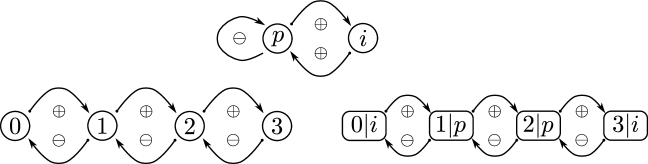
Figure 13: The allowed transitions for the one-dimensional $p$-$i$ (top) and $Q$-charge (left) models. There is a 2-1 graph homomorphism from the $Q$-charge finite-state graph to that of the $p$-$i$ model — namely map the nodes $0,3$ to the node $i$ and the nodes $1,2$ to the node $p$.

The one-dimensional counterpart to this conjecture can be proved quite readily:

Theorem 4.

For the one-dimensional lattice,

$$\kappa_{charge(3)} =\kappa_{even}=\frac{1+\sqrt{5}}{2}.$$ (35)

Proof:

Perhaps the most obvious way to demonstrate this is to construct the appropriate transfer matrices for the $Q$-charge and $p$-$i$ models (see Fig. 13). These are

$$V_{\mbox{\scriptsize$p$-$i$ }} =\begin{pmatrix}1&1\\ 1&0\end{pmatrix} V_{\mbox{\scriptsize$Q$-charge}} =\begin{pmatrix}0&1&0&0\\ 1&0&1&0\\ 0&1&0&1\\ 0&0&1&0\end{pmatrix}.$$ (36)

A quick computation shows that the dominant eigenvalue (and hence the growth rate) of each is $\frac{1+\sqrt{5}}{2}$.

It is more instructive, however, to construct a mapping between the two states-on-bonds models. This mapping is a $2$-$1$ graph homomorphism between the two underlying state graphs as illustrated in Fig. 13. Simply map the vertices labelled by $0,3$ to the vertex labelled $i$, and the vertices labelled $1,2$ to the vertex labelled $p$.

Now consider any valid $Q$-charge configuration in one dimension. Using the above mapping we can transform it into a valid $p$-$i$ configuration. The reverse mapping is $1$ to $2$. To see this pick a single $p$ in the $p$-$i$ configuration — we may choose whether this maps to a $1$ or a $2$ in the corresponding $Q$-charge configuration. Once this choice is made, the rest of the mapping is fixed. The result follows. ∎

The mapping used in the above proof can also be used to show that the growth rate of the charge(3) model in two dimensions is at least that of the even model.

Theorem 5.

For the two-dimensional lattice,

$$\kappa_{charge(3)} \geq\kappa_{even}(\geq 1.357\,587\,502\,184\,123).$$ (37)

Proof:

Choose any bond on the lattice, and draw a line parallel to $y=x$ through this bond. Choose all bonds intersecting this line to have $Q$-charge states 0 or 2, as shown in Fig. 14. Now consider a valid $Q$-charge configuration conforming to these restrictions. The set of such configurations is a (strict) subset of all valid $Q$-charge configurations. However, since the bond-states must increase or decrease by 1 as we read across horizontal and vertical lines, we have determined the parity of every bond state on the lattice.

Figure 14: Restriction for the $Q$-charge $\leftrightarrow$ $p$-$i$ mapping. All states on the red line must have state 0 or 2 in the $Q$-charge model.

Now in every cell, the parities of the N and W bonds are determined and identical. A full enumeration of the (five) possible cell configurations shows that in this case, the above mapping between the $Q$-charge and $p$-$i$ models is a bijection between all valid $Q$-charge and $p$-$i$ cell configurations. Thus the number of configurations for each model is the same. Since we have only taken a subset of valid $Q$-charge configurations, but all valid $p$-$i$ configurations, this provides the inequality. ∎

Unfortunately, we have not been able to prove the reverse inequality, though we can make a non-rigorous argument as to why this should be so. In every $Q$-charge configuration, there will be a number of faces where the N and W bonds have identical parity (the ‘good’ faces), and a number of faces where the N and E bonds have the same parity (the ‘bad’ faces). As mentioned above, it is possible to take configurations which consist entirely of good faces, and these are equivalent to the $p$-$i$ configurations.

It is also possible to take configurations which consist entirely of bad faces, and a similar analysis of cell configurations shows that these faces map onto (invalid) $p$-$i$ faces containing exactly one $i$ and three $p$’s. By considering an $i$ as an ‘occupied’ bond and a $p$ as an ‘vacant’ bond, we see that these configurations are in fact fully-packed dimer configurations. The growth rate of such configurations has been proved [31] to be

$$\kappa =e^{Catalan/\pi}=1.338\,515\,15\dots$$ (38)

which is less than our proved lower bound for $\kappa_{even}$. Therefore, these configurations are exponentially infrequent in the set of $Q$-charge configurations.

Another possibility is to take configurations where the good faces and bad faces are arranged in a checkerboard pattern. We call this model the ‘elbow’ model, due to the characteristic shape of the individual bond configurations. The growth rate of this model can be rigorously bounded above using the method of Calkin and Wilf [2]. Using transfer matrices of width $8$, we calculate $\kappa_{elbow}\leq 1.333\,521\ldots$, which is again less than the proved lower bound for $\kappa_{even}$.

Now choose any fixed set of parities for the rows and columns of the lattice. In these configurations, the good faces and bad faces form a ‘tartan’-like configuration (see Fig. 15). The growth rate of such configurations is some combination of the growth rates of the even model (the good faces), the fully-packed dimer model (the bad faces) and the elbow model (an interfacial term between good and bad faces). Out of these three models, the even model has the largest growth rate and so the growth rate of such configurations cannot be greater than $\kappa_{even}$.

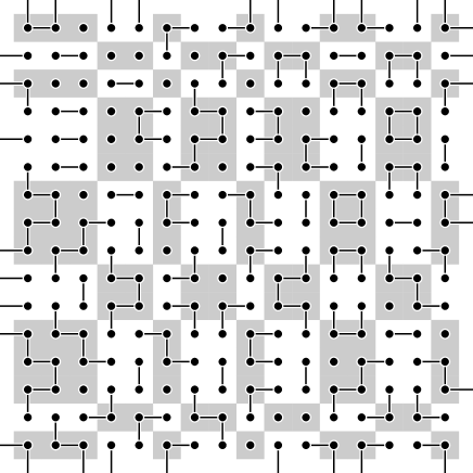
Figure 15: An example of the $Q$-charge model mapped to a ‘tartan’ combination of $p$-$i$ and fully-packed dimer constraints. The shaded regions obey the $p$-$i$ constraint, while the unshaded regions obey the dimer constraint.

Now there are $2^{2\sqrt{N}}$ ways to choose these parities on a lattice of $N$ spins, a sub-exponential factor. Each of these ways results in a growth rate not more than $\kappa_{even}$, and therefore the set of all valid $Q$-charge configurations has a growth rate not greater than $\kappa_{even}$.

This (admittedly non-rigorous) argument, combined with the accuracy of our numerical results and the above theorem, presents what we find to be a compelling case that $\kappa_{charge(3)}=\kappa_{even}$.

VI Conclusion

In this paper, we have constructed very accurate rigorous lower bounds on the growth rate of several families of data storage models: exclusion, colouring, even, and charge(3) models. The process we use also gives us very precise estimates of the growth rates. This is achieved using Baxter’s corner transfer matrix formalism combined with the corner transfer matrix renormalisation group method of Nishino and Okunishi.

The precision of our bounds allows us to conjecture the equality of the growth rate of two of our models, the charge(3) and even models. We have proved one inequality for this relation, and have a non-rigorous (but overall convincing) argument for equality.

For future work, we would like to be able to construct upper bounds of similar quality. The quality of proved lower bounds have typically been much higher than that of upper bounds. It may be possible to use linear algebra results to obtain a bound on the error of our estimates, and so derive an upper bound for the growth rate. It certainly is possible to bound the distance between our estimate and the nearest eigenvalue of the transfer matrix using a theorem of Wilkinson [32]. However, there is no guarantee that this eigenvalue is the dominant eigenvalue, and so more work needs to be done to establish a provable upper bound.

In addition, there are still a number of constraints which we have not analysed in this paper, for example higher-order charge or colouring models. These are amenable to identical analysis, and are the subject of future work.

References

- [1] K. Engel, “On the Fibonacci number of an lattice,” Fibonacci Quarterly, vol. 28, no. 1, pp. 72–78, 1990.
- [2] N. Calkin and H. Wilf, “The number of independent sets in a grid graph,” SIAM J. Disc. Math., vol. 11, no. 1, pp. 54–60, 1998.
- [3] E. Louidor and B. Marcus, “Improved lower bounds on capacities of symmetric 2D constraints using Rayleigh quotients,” IEEE Trans. Inf. Theory, vol. 56, no. 4, pp. 1624–1639, 2010.
- [4] R. J. Baxter, “Dimers on a rectangular lattice,” J. Math. Phys., vol. 9, p. 650, 1968.
- [5] ——, “Variational approximations for square lattice models in statistical mechanics,” J. Stat. Phys., vol. 19, no. 5, pp. 461–478, 1978.
- [6] R. J. Baxter, I. G. Enting, and S. K. Tsang, “Hard-square lattice gas,” J. Stat. Phys., vol. 22, no. 4, pp. 465–489, 1980.
- [7] R. J. Baxter, “Hard hexagons: exact solution,” J. Phys. A: Math. Gen., vol. 13, p. L61, 1980.
- [8] ——, Exactly solved models in statistical mechanics. Academic Press London, 1982.
- [9] T. Nishino and K. Okunishi, “Corner transfer matrix renormalization group method,” J. Phys. Soc. Jpn., vol. 65, no. 4, pp. 891–894, 1996.
- [10] ——, “Corner transfer matrix algorithm for classical renormalization group,” J. Phys. Soc. Jpn., vol. 66, no. 10, pp. 3040–3047, 1997.
- [11] S. White, “Density matrix formulation for quantum renormalization groups,” Physical Review Letters, vol. 69, no. 19, p. 2863, 1992.
- [12] U. Schollwöck, “The density-matrix renormalization group,” Rev. Mod. Phys., vol. 77, no. 1, p. 259, 2005.
- [13] D. P. Foster and C. Pinettes, “A corner transfer matrix renormalization group investigation of the vertex-interacting self-avoiding walk model,” J. Phys. A: Math. Gen., vol. 36, pp. 10 279–10 298, 2003.
- [14] V. V. Mangazeev, M. T. Batchelor, V. V. Bazhanov, and M. Y. Dudalev, “Variational approach to the scaling function of the 2d ising model in a magnetic field,” J. Phys. A: Math. Theor., vol. 42, p. 042005, 2009.
- [15] Y. Chan, “Series expansions from the corner transfer matrix renormalization group method: the hard squares model,” J. Phys. A: Math. Theor., vol. 45, p. 085001, 2012.
- [16] R. J. Baxter, “Planar lattice gases with nearest-neighbor exclusion,” Ann. Comb., vol. 3, no. 2, pp. 191–203, 1999.
- [17] M. Cohn, “On the channel capacity of read/write isolated memory,” Disc. Appl. Math., vol. 56, no. 1, pp. 1–8, 1995.
- [18] M. Golin, X. Yong, Y. Zhang, and L. Sheng, “New upper and lower bounds on the channel capacity of read/write isolated memory,” in Information Theory, 2000. Proceedings. IEEE International Symposium on. IEEE, 2000, p. 280.
- [19] W. Weeks IV and R. E. Blahut, “The capacity and coding gain of certain checkerboard codes,” IEEE Trans. Inf. Theory, vol. 44, no. 3, pp. 1193–1203, 1998.
- [20] N. L. Biggs, “Colouring square lattice graphs,” Bull. London Math. Soc, vol. 9, pp. 54–56, 1977.
- [21] R. Shrock and S.-H. Tsai, “Lower bounds and series for the ground-state entropy of the Potts antiferromagnet on Archimedean lattices and their duals,” Phys. Rev. E, vol. 56, pp. 4111–4124, Oct 1997. [Online]. Available: http://link.aps.org/doi/10.1103/PhysRevE.56.4111
- [22] P. H. Lundow and K. Markström, “Exact and approximate compression of transfer matrices for graph homomorphisms,” LMS J. Comput. Math, vol. 11, pp. 1–14, 2008.
- [23] J. Jacobsen, “Bulk, surface and corner free-energy series for the chromatic polynomial on the square and triangular lattices,” J. Phys. A: Math. Theor., vol. 43, p. 315002, 2010.
- [24] E. H. Lieb, “Exact solution of the problem of the entropy of two-dimensional ice,” Phys. Rev. Lett., vol. 18, pp. 692–694, Apr 1967. [Online]. Available: http://link.aps.org/doi/10.1103/PhysRevLett.18.692
- [25] D. P. Foster and C. Pinettes, “Corner-transfer-matrix renormalization-group method for two-dimensional self-avoiding walks and other models,” Phys. Rev. E, vol. 67, no. 045105, 2003.
- [26] G. Guennebaud, B. Jacob et al., “Eigen v3,” http://eigen.tuxfamily.org, 2010.
- [27] L. Fousse, G. Hanrot, V. Lefèvre, P. Pélissier, and P. Zimmermann, “MPFR: A multiple-precision binary floating-point library with correct rounding,” ACM Transactions on Mathematical Software, vol. 33, no. 2, pp. 13:1–13:15, Jun. 2007. [Online]. Available: http://doi.acm.org/10.1145/1236463.1236468
- [28] K. Okunishi, Y. Hieida, and Y. Akutsu, “Universal asymptotic eigenvalue distribution of density matrices and corner transfer matrices in the thermodynamic limit,” Phys. Rev. E, vol. 59, no. 6, pp. R6227–R6230, 1999.
- [29] S. Friedland, P. H. Lundow, and K. Markström, “The 1-vertex transfer matrix and accurate estimation of channel capacity,” IEEE Trans. Inf. Theory, vol. 56, no. 8, pp. 3692–3699, 2010.
- [30] J. Borwein, P. Borwein, and S. Plouffe, “Inverse symbolic calculator,” http://isc.carma.newcastle.edu.au/.
- [31] P. Kasteleyn, “Dimer statistics and phase transitions,” J. Math. Phys., vol. 4, no. 2, p. 287, 1963.
- [32] J. H. Wilkinson, “Rigorous error bounds for computed eigensystems,” The Computer Journal, vol. 4, no. 3, pp. 230–241, 1961.