Dark Breathers in Granular Crystals

Abstract

We present a study of the existence, stability and bifurcation structure of families of dark breathers in a one-dimensional uniform chain of spherical beads under static load. A defocusing nonlinear Schrödinger equation (NLS) is derived for frequencies that are close to the edge of the phonon band and is used to construct targeted initial conditions for numerical computations. Salient features of the system include the existence of large amplitude solutions that bifurcate with the small amplitude solutions described by the NLS equation, and the presence of a nonlinear instability that, to the best of the authors knowledge, has not been observed in classical Fermi-Pasta-Ulam lattices. Finally, it is also demonstrated that these dark breathers can be detected in a physically realistic way by merely actuating the ends of an initially at rest chain of beads and inducing destructive interference between their signals.

PACS numbers

63.20.Ry, 63.20.Pw, 45.70.-n, 46.40.-f

I Introduction

Granular crystals, which consist of closely packed arrays of elastically interacting particles, have sparked recent theoretical and experimental interest. On one hand, the relevant mathematical model is difficult to analyze due to, among other things, the lack of smoothness of the corresponding potential function, calling for new ideas to study this nonlinear lattice problem pego ; atanas . On the other hand, the ability to conduct experiments for a wide range of setups, including chains consisting of beads of various geometries and masses, nonlinearity strength, and even dimension nesterenko1 ; sen08 ; nesterenko2 ; coste97 , make the subject of granular crystals exciting for its potential relevance in applications including shock and energy absorbing layers dar06 ; hong05 ; fernando ; doney06 , actuating devices dev08 , acoustic lenses Spadoni , acoustic diodes china ; Nature11 and sound scramblers dar05 ; dar05b , to name a few.

One fundamental structure known to exist in granular crystals is the so-called intrinsic localized mode, or discrete breather. Discrete breathers are time-periodic solutions of the underlying equations of motion which are localized in space. Generally speaking, they are well studied, and are known to exist in a host of nonlinear lattice models Flach2007 . The most commonly studied breather is one with tails decaying to zero, which is often referred to as a bright breather. The term “bright” is used, as the solution can be viewed as a discrete carrier wave with amplitudes modulated by a bright soliton. It is then natural to consider a discrete wave modulated by a dark soliton, which is then in turn called a dark breather, see Fig. 1 for an example. Although bright discrete breathers are known to exist in granular crystals (in dimer or higher periodic configurations, and in monomer chains with defects for example Theo2009 ; Theo2010 ; Boechler2009 ; hooge11 ), the properties of dark discrete breathers remains an open question, and is the subject of this work.

It should be highlighted here that in monomer i.e., homogeneous chains (for which, there is purely an acoustic band), the conditions established for the bifurcation of discrete breathers Flach2007 do not allow the bifurcation of bright breathers. For that reason the latter have only been identified in heterogeneous configurations with different periodicities Theo2010 ; Boechler2009 ; hooge11 , or in monomer settings bearing defects Theo2009 , where the localization is not intrinsic to the chain but rather is supported as an impurity mode by the defect. The only possibility that exists in the homogeneous chain, under static load (i.e., in the linearizable limit) for intrinsic localization may arise in the form of the dark breathers proposed herein. For this reason, we believe that such states are fundamental ones in the study of granular systems and merit an investigation of their existence properties, linear and nonlinear stability, as well as of their dynamics. These topics form the focus of the present work which is structured as follows. In section 2, we present the general properties of the model. In section 3, we analyze the model near the band edge of its linear acoustic spectrum, and derive a defocusing nonlinear Schrödinger equation characterizing its envelope dynamics. In section 4, we specify the finite dimensional lattice dynamical system to be studied and its bifurcation analysis is carried out in section 5. While sections 6 and 8 consider variants of the center position of the breather and of the associated boundary conditions, section 7 focuses on the linear stability properties of the states. Section 9 analyzes the validity of the analytical approximation, while section 10 makes connections with current experimental settings, presenting a scheme for the potential realization of the dark breathers. Finally, section 11 presents our conclusions and some challenges for future work.

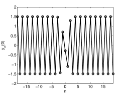
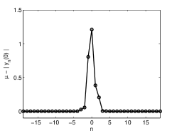
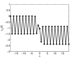
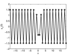
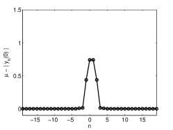
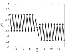
Figure 1: Top: A site-centered dark breather solution with $\omega_{b}=1.9$ in the strain variable $y_{n}=u_{n+1}-u_{n}$ (left), renormalized strain variable $\mu-|y_{n}|$, where $\mu$ is the breather amplitude (middle) and in displacement variables $u_{n}$ (right). The markers indicate where the solution takes values on the lattice. The solid line is shown for clarity. Bottom: Same as top row but for the bond-centered solution.

II Model

The model describing the dynamics of a one dimensional (1D) homogeneous chain of spherical beads is given by nesterenko1 ; coste97 :

$$M\ddot{u}_{n}=V_{\mathrm{GC}}^{\prime}(u_{n}-u_{n-1})-V_{\mathrm{GC}}^{\prime}(u_{n+1}-u_{n}),$$ (1)

with,

$$V_{\mathrm{GC}}^{\prime}(x)=A\left[\delta_{0}-x\right]_{+}^{3/2},$$ (2)

where $n\in I$, with $I$ a countable index set, $u_{n}=u_{n}(t)\in{\mathbb{R}}$ is the displacement of the $n$-th bead from equilibrium position at time $t$, $A$ is a material parameter (depending on the elastic properties of the material and the geometric characteristics of the beads nesterenko1 ), $M$ is the bead mass and $\delta_{0}$ is an equilibrium displacement induced by a static load $F_{0}=A\delta_{0}^{3/2}$. The bracket is defined by $[x]_{+}=\mathrm{max}(0,x)$. Equation (1) with $I={\mathbb{Z}}$ has the Hamiltonian,

$$H=\sum_{n\in{\mathbb{N}}}\frac{1}{2}Mv_{n}^{2}+V_{\mathrm{GC}}(u_{n+1}-u_{n}),$$

where $v_{n}=\dot{u}_{n}$. Considering small amplitude solutions, i.e.,

$$\frac{|u_{n-1}-u_{n}|}{\delta_{0}}\ll 1,$$

implies that we can Taylor expand $V_{\mathrm{GC}}^{\prime}(x)$ . Keeping terms up to fourth order yields an approximate model,

$$M\ddot{u}_{n}=V_{\mathrm{FPU}}^{\prime}(u_{n+1}-u_{n})-V_{\mathrm{FPU}}^{\prime}(u_{n}-u_{n-1}),$$ (3)

where

$$V_{\mathrm{FPU}}^{\prime}(x)=K_{2}x+K_{3}x^{2}+K_{4}x^{3},$$

and

$$K_{2}=\frac{3}{2}A\delta_{0}^{1/2},\quad K_{3}=-A\frac{3}{8}\delta_{0}^{-1/2},\quad K_{4}=-A\frac{3}{48}\delta_{0}^{-3/2}.$$ (4)

Equation (3) is an example of the well studied Fermi-Pasta-Ulam (FPU) model. It is has been shown by James James01 ; James03 (see also the discussion in Flach2007 ) that small amplitude bright breathers exist in the FPU model for frequencies above the phonon band if and only if $B:=3K_{2}K_{4}-4K_{3}^{2}>0$. For coefficients such that $B<0$, small amplitude dark breathers were shown to exist for frequencies within the phonon band. The coefficients (4) associated to the granular crystal model correspond to $B<0$, and thus the existence results for dark breathers can be carried over for sufficiently small amplitudes (see e.g. Theorem 5 of James03 ).

In this paper, we begin with small amplitude solutions, where the phenomenology of the FPU lattice and granular crystal lattice are very similar. However, we will see that as we depart from the familiar small amplitude limit, a host of new phenomena will emerge that are particular to the monomer granular crystal model and its rather special nonlinearity bearing the unusual $3/2$ power, but also the tensionless characteristic (namely, that there is only force between the beads when they are in contact).

III Derivation of the defocusing NLS equation in the strain variable formulation

It is more natural to derive the nonlinear Schrödinger equation in terms of the strain variable $y_{n}=u_{n+1}-u_{n}$. We note that for a finite chain, a displacement variable solution can be recovered using the relation,

$$u_{n}=u_{1}+\sum_{j=1}^{n-1}y_{j},$$ (5)

where an arbitrary choice for the first node must be made. Equation (1) has the following form in the strain variables,

$$M\ddot{y}_{n}=-V_{\mathrm{GC}}^{\prime}(y_{n+1})+2V_{\mathrm{GC}}^{\prime}(y_{n})-V_{\mathrm{GC}}^{\prime}(y_{n-1}).$$ (6)

The FPU equation can again be derived, yielding,

$$M\ddot{y}_{n}=V_{\mathrm{FPU}}^{\prime}(y_{n+1})-2V_{\mathrm{FPU}}^{\prime}(y_{n})+V_{\mathrm{FPU}}^{\prime}(y_{n-1}).$$ (7)

The linear problem (i.e. when $K_{3}=K_{4}=0$) is solved by,

$$y_{n}(t)=y_{no}e^{i(kn+\omega t)},$$

for all $k\in{\mathbb{R}}$ where $\omega$ and $k$ are related through the dispersion relation,

$$\omega(k)^{2}=4K_{2}/M\sin^{2}(k/2),$$

such that the cutoff point of the phonon band is $2\sqrt{K_{2}/M}$.

Consider the standard NLS multiple scale ansatz, which up to first order has the form,

$$y_{n}(t)\approx\psi_{n}(t):=\varepsilon A(X,T)e^{i(k_{0}n+\omega_{0}t)}+\mathrm{c.c.}\,,\quad X=\varepsilon(n+ct),\quad T=\varepsilon^{2}t,$$ (8)

where $\varepsilon\ll 1$ is a small parameter, effectively parameterizing the solution amplitude (and also its inverse width). The substitution of this ansatz into (7) and equation of the various orders of $\varepsilon$ leads to the dispersion relation $\omega_{0}=\omega(k_{0})$, the group velocity relation $c=\omega^{\prime}(k_{0})$, and the nonlinear Schrödinger equation,

$$i\partial_{T}A(X,T)+\nu_{2}\partial_{X}^{2}A(X,T)+\nu_{3}A(X,T)|A(X,T)|^{2}=0,$$ (9)

where $\nu_{2}=-\omega^{\prime\prime}(k_{0})/2>0$ and

$$\nu_{3}=\frac{K_{3}^{2}}{K_{2}^{2}}\tilde{\gamma}+\frac{3K_{4}}{2K_{2}}\omega(k_{0}),$$ (10)

while

$$\tilde{\gamma} = \frac{\omega(k_{0})}{2}\left(\frac{\omega(2k_{0})}{2\omega(k_{0})-\omega(2k_{0})}-\frac{\omega(2k_{0})}{2\omega(k_{0})+\omega(2k_{0})}\right.$$

$$\left.\qquad\qquad+\frac{2\omega^{\prime}(0)}{\omega^{\prime}(k_{0})-\omega^{\prime}(0)}-\frac{2\omega^{\prime}(0)}{\omega^{\prime}(k_{0})+\omega^{\prime}(0)}\right).$$

Full details of the derivation of the NLS equation starting from the homogeneous FPU equation, including the higher order terms of the ansatz, can be found e.g. in Schn10 . Since we seek standing wave solutions, we choose the wavenumber to be at the edge of the phonon band $k_{0}=\pi$, such that the group velocity vanishes, $\omega_{0}=2\sqrt{K_{2}/M}$, and

$$\left.\nu_{3}\right|_{k_{0}=\pi}=3K_{2}K_{4}-4K_{3}^{2}=B.$$

We already noted that $B<0$ (and hence $\nu_{3}<0$) for coefficients defined in (4). Thus, the NLS equation (9) is defocusing. Steady states of (9) have the form,

$$A(X,T)=\tilde{A}(X)e^{i\kappa T},$$

where $\kappa\in{\mathbb{R}}$ and $\tilde{A}(X)$ satisfies the Duffing equation,

$$\partial_{X}^{2}\tilde{A}=-\frac{1}{\nu_{2}}\left(|\kappa|\tilde{A}-|\nu_{3}|\tilde{A}^{3}\right),$$ (12)

where $\kappa<0$. Equation (12) possesses heteroclinic solutions which have the form,

$$\tilde{A}(X)=\sqrt{\kappa/\nu_{3}}\tanh\left(\sqrt{\frac{-\kappa}{2\nu_{2}}}(X-X_{0})\right).$$

Reconstructing the original solution from our ansatz of Eq. (8), we have the following approximation,

$$y_{n}(t) \approx \varepsilon\tilde{A}e^{i\kappa T}e^{i(k_{0}n+\omega_{0}t)}+\mathrm{c.c.}$$

$$= 2\varepsilon(-1)^{n}\sqrt{\frac{\kappa}{\nu_{3}}}\tanh\left(\sqrt{\frac{-\kappa}{2\nu_{2}}}\varepsilon(n-x_{0})\right)\cos(\omega_{b}t)\quad\quad\quad(\mathrm{for}\,\,k_{0}=\pi)$$

where $\omega_{b}=\omega_{0}+\kappa\varepsilon^{2}$ is the frequency of the breather, $\kappa<0$ is a fixed but arbitrary parameter and $X_{0}=\varepsilon x_{0}$ is an arbitrary spatial translation. When $\kappa<0$, the frequency of the breather lies within the phonon band. We note that the same approximation (up to first order) can be obtained by performing a center manifold reduction (see e.g. James01 ; Rey04 with $\kappa=-\nu_{2}$, $\varepsilon=\sqrt{-\mu}$ and $A=M=1$ such that $\nu_{2}=1/4$). It is relevant to mention that the defocusing NLS equation can also be derived in the displacement variable formulation Huang .

If $\nu_{3}>0$ (which is not possible here), then one would need $\kappa>0$, which, in turn, would result in the existence of homoclinic solutions and thus of bright breathers with frequencies above the phonon band.

IV The finite dimensional system and its conservation laws

The boundary conditions (BCs) of the finite dimensional system used for the numerical simulations will play an important role since the dark breathers have non-decaying tails. In terms of the strain variable, a logical choice is a periodic boundary condition $y_{0}=y_{N}$ , $y_{N+1}=y_{1}$. To check our numerical results, we also carry out simulations in the displacement variables. The following system of $N+1$ equations is consistent with the system in the strain variable representation and periodic boundary conditions,

$$M\ddot{u}_{1} = A(\delta_{0}-(u_{N+1}-u_{N}))^{3/2}_{+}-A(\delta_{0}-(u_{2}-u_{1}))^{3/2}_{+},$$

$$M\ddot{u}_{n} = A(\delta_{0}-(u_{n}-u_{n-1}))^{3/2}_{+}-A(\delta_{0}-(u_{n+1}-u_{n}))^{3/2}_{+},\quad n\in\{2,N\}$$

$$M\ddot{u}_{N+1} = A(\delta_{0}-(u_{N+1}-u_{N}))^{3/2}_{+}-A(\delta_{0}-(u_{2}-u_{1}))^{3/2}_{+},$$

The redundancy of the last equation implies $\ddot{u}_{N+1}=\ddot{u}_{1}$, such that the above may be written as a system of $N$ equations,

$$M\ddot{u}_{1} = A(\delta_{0}-(u_{1}+c_{1}t+c_{2}-u_{N}))^{3/2}_{+}-A(\delta_{0}-(u_{2}-u_{1}))^{3/2}_{+},$$

$$M\ddot{u}_{n} = A(\delta_{0}-(u_{n}-u_{n-1}))^{3/2}_{+}-A(\delta_{0}-(u_{n+1}-u_{n}))^{3/2}_{+},\quad n\in\{2,N-1\}$$

$$M\ddot{u}_{N} = A(\delta_{0}-(u_{N}-u_{N-1}))^{3/2}_{+}-A(\delta_{0}-(u_{1}+c_{1}t+c_{2}-u_{N}))^{3/2}_{+},$$

where $c_{1}=\dot{u}_{N+1}(0)-\dot{u}_{1}(0)$ and $c_{2}={u}_{N+1}(0)-{u}_{1}(0)$. This system maintains the conserved quantities of the infinite system. For example, if $c_{1}=0$, then the Hamiltonian and mechanical momentum,

$$H=\sum_{n=1}^{N-1}\left[\frac{1}{2}Mv_{n}^{2}+V_{\mathrm{GC}}(u_{n+1}-u_{n})\right]+V_{\mathrm{GC}}(u_{1}+c_{2}-u_{N}),\quad\quad P=\sum_{n=1}^{N}Mv_{n},$$

are conserved respectively. The conservation of the Hamiltonian is connected to the temporal translation invariance $t\rightarrow t+\delta t$ and the conservation of momentum is a result of the vertical translation invariance $u=u+\delta u$. An interesting feature is the invariance,

$$u_{n}\rightarrow\alpha u_{n}+cn,\quad\quad t\rightarrow\alpha^{-1/4}t,\quad\quad\alpha=(\delta_{0}-c)/\delta_{0},$$ (13)

which holds in the infinite and finite lattice using the above mentioned boundary conditions. This last invariance is connected with the existence of a marginal mode and it has important consequences in the linear stability analysis described in Sec. VII.

V Bifurcations

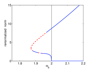
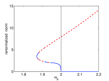
Figure 2: Left: Renormalized $l^{2}$ norm of the site-centered solution versus $\omega_{b}$ with a vertical center of $c=0$. The vertical line shows the edge of the phonon band $\omega=2$. The upper branch of the curve reaches past the edge of the phonon band and increases indefinitely. Right: Same as left, but for the bond-centered solution. Regions where a real instability is present are indicated by a dashed red line (see Sec. VII for details).

We compute numerically exact dark breather solutions using a Newton-type solver for time-periodic solutions (see e.g. Flach2007 for details). We carry out the computations in the strain variables with periodic boundary conditions with a lattice size of $N=51$. The associated Jacobian matrix is rank deficient due to the invariances of the system, and therefore an additional constraint is needed. It is sufficient to fix the vertical center of the solution,

$$c:=\frac{\sup_{t\in[0,T_{b}]}y_{1}(t)+\inf_{t\in[0,T_{b}]}y_{1}(t)}{2},$$

where $T_{b}=2\pi/\omega_{b}$ is the breather period. For all reported results we used the parameter values $M=\delta_{0}=1$ and $A=2/3$ such that $\omega_{0}=2$. After a rescaling of time and amplitude, solutions for arbitrary parameter values can be recovered. The $l^{2}$ norm and energy of the dark breathers will depend on the nonzero background of the solutions. Thus, to measure the solutions we consider the renormalization Kivshar94 ,

$$\tilde{y}_{n}=\mu-|y_{n}-c|\quad\quad\quad\|y_{n}\|_{\tilde{l}^{2}}=\sum_{n\in I}\mu^{2}-|y_{n}-c|^{2},$$

where $\mu$ is defined as the amplitude of the breather,

$$\mu:=\frac{\sup_{t\in[0,T_{b}]}y_{1}(t)-\inf_{t\in[0,T_{b}]}y_{1}(t)}{2}.$$

The renormalized profiles can be seen in the middle panels of Fig. 1. We use the analytical approximation (8) to seed the numerical solver. Ansatz (8) with $x_{0}=0$ represents a so-called site-centered solution (see Fig. 1 top) whereas the bond-centered solution corresponds to $x_{0}=0.5$ (see Fig. 1 bottom).

In the finite lattice, eigenvectors of the equations of motion linearized about the trivial solution also provide an option for an initial seed. The largest computed eigenvalue $\omega$ of the linear spectrum serves as the numerical cutoff value of the frequency (which is slightly smaller than the exact value of $\omega_{0}$ but approaches it as $N\rightarrow\infty$). The eigenvector of the $N-1$ eigenvalue has the profile of a dark breather. The drawback of using the linearized solution is that there is no information regarding the correct amplitude. For this reason, we use (8) for the initial seed, which approximates both the shape and amplitude of the solution.

In the left panel of Fig. 2, we show the renormalized $l^{2}$ norm of the numerically exact site-centered dark breathers. The solutions do not exist for arbitrarily small $\omega_{b}$ but rather, there is a fold at $\omega_{b}\approx 1.87$. However, we note here that this is a fold in the particular parameters which does not constitute a point of change in the spectral stability of the observed states. The top branch persists past the edge of the phonon band $\omega_{0}=2$, with indefinitely increasing amplitude. For this reason, the solutions making up the top branch in the figure can be thought of as strongly nonlinear solutions, and those making up the bottom branch as weakly nonlinear solutions. A red dashed line indicates that the solution possesses a real instability, a blue solid line indicates the solution does not (see Sec. VII for more details).

VI Dark breathers with a nonzero center

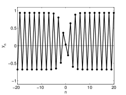
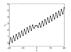
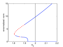
Figure 3: Left: A site-centered dark breather solution with $\omega_{b}=1.9$ and a nonzero center $c=0.13$ in the strain variable $y_{n}$. Middle: The same solution but in the displacement variables $u_{n}$. Right: Renormalized $l^{2}$ norm of the site-centered solution versus $\omega_{b}$ with a vertical center of $c=0.13$. The vertical line shows the edge of the phonon band $\omega=2$. In contrast to the $c=0$ case shown in Fig. 2, the bottom branch terminates at a value below the edge of the phonon band.

The equations of motion for both the infinite system and the finite system with periodic BCs are invariant under the transformation

$$y_{n}\rightarrow y_{n}\alpha+c,\quad\quad t\rightarrow\alpha^{-1/4}t,\quad\quad\alpha=(\delta_{0}-c)/\delta_{0},$$ (14)

where (14) is merely the strain variable equivalent of (13). Thus, there is an entire family of solutions associated with the vertical shift $c$. We note that a similar transformation has been introduced in Rey04 for the case of FPU lattices. Figure 3 shows an example of a dark breather with $c=0.13$ in the strain (left) and displacement variables (middle). The bifurcation diagram (right) is similar to its $c=0$ counterpart, but is shifted in the $\omega$ axis where the cutoff point is $\omega_{0}\alpha^{1/4}=2\alpha^{1/4}$. The invariance (14) can also be used as another accuracy check for the numerical simulations. We can choose the value of the constraint $c$ in the Newton method and test if it converges to the appropriate solution as predicted by (14), assuming we have computed the $c=0$ solution. Naturally, the stability of the two solutions also has the same structural characteristics, as regards intervals with real Floquet multipliers.

Note that a constant vertical shift $y\rightarrow y+c$ is the same as leaving $y$ unchanged and changing the precompression $\delta_{0}\rightarrow\delta_{0}-c$. Thus, all forthcoming discussions of changes in vertical center can be thought of as changes in precompression. For this reason it is clear that both the strongly and weakly nonlinear branch go toward the zero solution as the precompression goes to zero, since $\alpha\rightarrow 0$ as $c\rightarrow\delta_{0}$.

VII Linear stability analysis

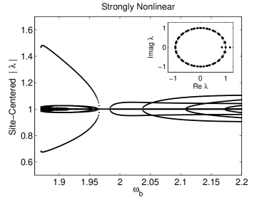
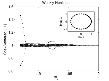
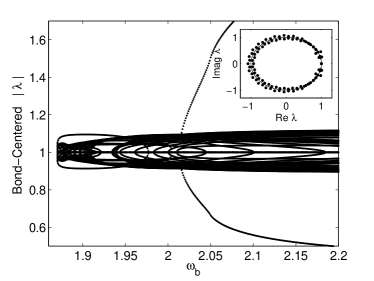
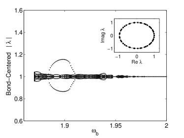
Figure 4: Floquet multipliers of the strongly (left) and weakly (right) nonlinear solutions with $c=0$ versus frequency $\omega$ for the site-centered (top) and bond-centered (bottom) types. The Floquet multipliers for $\omega_{b}=1.95$ in the complex plane are shown in the respective insets.

There is a rich theory for the stability properties of breathers in Hamiltonian systems Flach2007 ; Aubry06 ; Flach05 . Here, linear stability is determined in the standard way: A perturbation $V_{n}(t)$ is added to a breather solution and (6) is used to derive an equation describing the evolution of $V$. Keeping only linear terms in $V$ will result in a Hills’ equation with a time periodic coefficient of period $T_{b}$. Thus, the eigenvalues (or Floquet multipliers) of the associated variational matrix at $t=T_{b}$ determine the linear stability of the breather solution. Due to the Hamiltonian structure of the system, all Floquet multipliers must lie on the unit circle for the solution to be (marginally) stable, otherwise, the solution is unstable.

There are continuous arcs of spectrum on the unit circle (in the infinite lattice limit), which can be computed from the phonon band of (6). Although, in contrast to the bright breather case, these arcs are not simply $\exp(i\omega\,T_{b})$, where $\omega\in[-\omega_{0},\omega_{0}]$. This is due to the nonzero background of the solutions we are linearizing about. The isolated (point spectrum) multipliers must be computed numerically. If an isolated one is real and lies off the unit circle, then the solution possess a so-called real-instability (see Fig. 4, top left for an example). Oscillatory instabilities are also possible, where the multiplier has both real and imaginary parts (and the corresponding multipliers come in quartets). In FPU lattices, it is known that numerically computed eigenvalues may lie off the unit circle due to the truncation of the infinite lattice to a finite lattice Flach2007 ; Aubry06 . To determine if the instability is a finite size effect, a band analysis can be carried out Flach2007 . Such a computation is outside the scope of this work, but we did carry out numerical simulations for larger values of the lattice size $N$. We found that the oscillatory multipliers do approach the unit circle, but level off before reaching it. In other words, the oscillatory instabilities seem to be genuine, albeit weak.

Examples of the numerically computed Floquet spectrum of the site-centered and bond-centered solutions, for both strongly and weakly nonlinear types, are shown in the insets of Fig. 4 for $\omega_{b}=1.95$. The moduli of the Floquet multipliers are also shown for various frequencies where real and oscillatory instabilities are present. The real instabilities are the larger arcs in the figure. For each solution type, there is an intricate cascade of oscillatory instabilities, which can be best seen for the strongly nonlinear site-centered solution. The magnitude of the oscillatory instabilities is small relative to that of the real instabilities. Therefore, in the bifurcation diagram of Fig. 2 only real instabilities are indicated, although oscillatory instabilities may be present. In Fig. 5 the manifestation of an instability of the strongly nonlinear bond-centered solution for $\omega_{b}=2.5$ is shown, which is characteristic of the simulations carried out for the perturbed unstable solutions. It can be clearly seen that the instability essentially sets the dark breather state in motion, although it does not appear to correspond to a genuinely traveling breather.

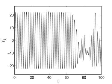
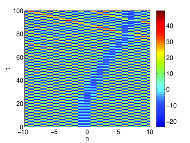
Figure 5: Manifestation of the real-instability of the strongly nonlinear bond-centered solution for $\omega_{b}=2.5$. The left panel shows the evolution of the $n=6$ node. The right panel is a contour plot of the time evolution of the entire solution. The color intensity corresponds to the value of the strain $y_{n}$. The checkered pattern is a consequence of the time periodicity of the solution. Notice the density dip of the solution near $n=0$, and how this structure re-arranges itself in a way reminiscent of a moving (dark breather) pattern after $t\approx 25$.

The linear stability analysis (LSA) described above can fail to describe instabilities that grow slower than exponentially Aubry06 . Such ”nonlinear” instabilities can emerge even if the linear stability analysis predicts the solution to be marginally stable. They are associated with degenerate eigenvalues (i.e. unit Floquet multipliers), although the presence of degenerate eigenvalues does not, in turn, guarantee the existence of a nonlinear instability. For solutions with $|y_{n}|<\delta_{0}$ there are, up to machine precision, six degenerate eigenvalues. One pair, corresponding to the phase mode $V_{p}=\{\dot{y}(0),\ddot{y}(0)\}$, is associated with the energy conservation/time reversal invariance of the system. The second pair associated to a pair of degenerate eigenvalues seems to be of the form $V_{t}=\{\partial y/\partial{x_{0}},\partial\dot{y}/\partial{x_{0}}\}$ which corresponds to continuous spatial translation invariance. This mode, called also ”translational” or ”pinning” mode, is of particular interest since it suggests that (exact) traveling dark breathers may exist in this model. Indeed for frequencies very close to the band edge, we found several intermediate solutions, which seem to be spatial translations of the same solution (i.e. solutions with various values of $x_{0}$ in Eq. (8)). For solutions with $|y_{n}|\geq\delta_{0}$ this invariance is lost, and there are only four degenerate eigenvalues in the linear stability problem.

The last pair of modes has the form $V_{c}=\{\partial y/\partial{c},\partial\dot{y}/\partial{c}\}$ where $c$ is the vertical center. To the best of the authors knowledge, these modes have never been found/examined in FPU lattices. Perturbing along the direction of these modes results in algebraic growth in the perturbation. Thus, we conjecture that there is a nonlinear instability associated with this marginal mode, (which in turn is connected to the shift invariance (14)). The heuristic argument for the presence of such an instability is as follows: if one chooses a small perturbation of the form $\varepsilon_{n}+c$, the dynamics of the solution with a vertical center of $c$ may emerge, which will have a lower frequency, due to (14). This is precisely what we observe in the numerical simulations with such perturbations. For example, the weakly nonlinear site-centered solution at $\omega_{b}=1.97$ is linearly stable. However a perturbation with initial value $V_{n}(0)=.01\max(y(0))(r_{n}+c)$, where $r_{n}$ is a random perturbation centered at 0 with $|r_{n}|<1$, will grow even though the LSA predicts that it should not. Moreover, the projection $p(t)=<y_{\mathrm{exact}}(\cdot,t)-y_{\mathrm{perturbed}}(\cdot,t),V_{c}>$ grows algebraically and is several orders of magnitude greater than the projections to the other linearization eigenvectors. This phenomenon is not observed when the above perturbation has $c=0$ for the identical timescale. Lastly, if the invariance (14) is absent, the nonlinear instability vanishes (see Sec. VIII for a relevant example).

We note in passing, that working on the equivalent displacement representation, see Sec.4, a fourth pair of Floquet multipliers is located at $(1,0)$ in the complex plane. This pair arises from the conservation of the total mechanical momentum.

VIII Other boundary conditions

Periodic boundary conditions are advantageous since the solution profiles closely resemble those of the infinite system, and invariances of the infinite system carry over to the finite case. However, other boundary conditions are also relevant and interesting to examine from an experimental point of view. The free boundary conditions $u_{0}:=u_{1}$ and $u_{N+1}:=u_{N}$ constitute such an example. In terms of strain variables, these become fixed boundary conditions $y_{0}=y_{N+1}=0$. The resulting profile resembles a multi-breather, see Fig. 6. This solution is no longer centered at zero. Unlike the periodic BC situation, one cannot normalize the solution to have a zero center, since the vertical shift invariance (14) is broken in the fixed BC system. Consequently, the corresponding marginal mode discussed in Sec.VII vanishes, along with the eigenvector $V_{c}$ and hence the nonlinear instability is absent in this case. Thus, choosing a strictly positive perturbation will no longer cause the integrator to shift towards a solution of a different frequency, since the corresponding family of vertically shifted solutions no longer exists. Indeed, in the simulations a perturbation of the form $\varepsilon_{n}+c$ induces the nonlinear instability in the periodic BC system, but the exact same perturbation in the fixed BC system does not lead to any instability and the corresponding dark breather is found to be structurally robust (where appropriate), in agreement with the perturbations of the linear stability analysis presented above.

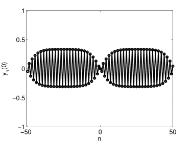
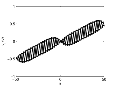
Figure 6: Left: A site-centered dark breather solution with $\omega_{b}=1.99$ in the strain variable $y_{n}$ with fixed boundary conditions $y_{0}=y_{N+1}=0$ with $N=101$. Right: The same solution but in the displacement variables $u_{n}$.

IX Accuracy of the NLS approximation

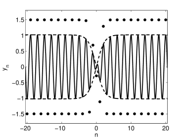
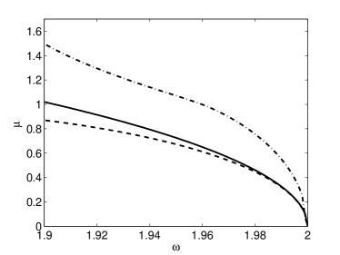
Figure 7: Left: Analytical approximation (solid line) with an envelope function that is the NLS dark soliton (dashed line), and a numerically exact dark breather (markers) for $\omega_{b}=1.9$ and $c=0$. Right: The amplitude of the NLS approximation (solid line), numerical breather with fixed $c=0$ (dashed-dot line) and numerical breather with varying $c$ (dashed line).

Although the NLS approximation (III) was sufficiently accurate to provide an initial seed for our numerical solver, it is relevant to investigate the extent to which the NLS approximation represents actual solutions to (6). Figure 7 shows a numerically exact solution in the strain variable (markers), the corresponding approximation (solid line) and the envelope (dashed line), which is defined by the NLS equation. From a visual inspection, the structure is quite proximal to the exact one, although the amplitude is underestimated. We also directly compared the amplitudes of the analytical prediction with the numerical solutions (right panel) for various $\omega_{b}$, where it can be seen that NLS approximation becomes irrelevant as $\omega_{b}$ moves away from the cutoff point $\omega=2$. It can perhaps be understood at an intuitive level, by inspecting Figure 7, that the NLS approximation is likely to be less successful for the dark breather states considered herein than the more standard case of the bright breathers Flach2007 . In the latter case, the solutions bifurcate from vanishing amplitude, on top of a vanishing background, while for the solutions considered herein the amplitude of the background is finite even close to the to the cutoff limit. Hence, the cubic nonlinearity approximation is expected to be less adequate even in the vicinity of that limit. Moreover, the fold bifurcation is not predicted by the NLS approximation and there is no approximation for the strongly nonlinear modes. Thus, the NLS approximation is only relevant for the weakly nonlinear solutions near the edge of the phonon band, as expected. It is interesting to point out that the amplitude of the dark breather with fixed $c=0$ is not the closest one to that of the NLS approximation.

The NLS approximation has been rigorously justified in the context of the FPU lattice in Schn10 , and more recently for an FPU equation with an arbitrary periodic configuration in CCPS12 . There, it can be shown that solutions with initial data defined by the NLS equation will remain close to an actual solution on long, but finite time scales, where the wavenumber $k$ can be arbitrarily chosen. However, those results do not apply to dark breathers, the issue being, as highlighted also above, the nonzero background. The results presented in this work suggest that the justification considered in these works may be an interesting topic to investigate in the context of granular crystals, but also perhaps more generally (even for smoother potentials) for dark breather states existing on a finite amplitude background.

X Exciting the dark breathers and dissipative effects

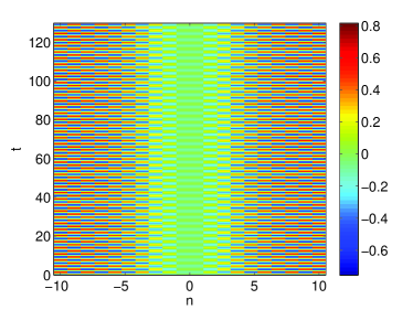
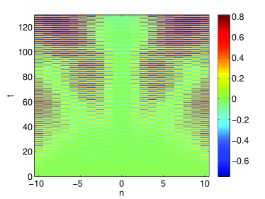
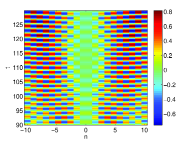
Figure 8: Top: contour plots of the space-time evolution of an exact weakly nonlinear, bond-centered dark breather with a vertical shift of $c=0$ and frequency $\omega_{b}=1.99$ (left) and an initially zero chain actuated out of phase at the boundaries with frequency $\omega_{b}=1.99$ (right). The color intensity corresponds to the strain $y_{n}$. Bottom: A zoom of the corresponding top panels between times $90$ and $130$.

In an experimental setting, it is difficult to impose an initial displacement and velocity to an arbitrary number of beads, and thus the exact solutions described above cannot be prescribed as an initial condition to the lattice. Hence, we have to resort to alternative approaches taking into consideration the somewhat limited actuation of the finite chain which is currently available experimentally. In that light, we propose an approach which relies solely on exciting (or actuating) the ends of a finite chain, and taking advantage of the resulting interference effect, in order to produce a time-periodic solution with a density dip (i.e., a dark breather).

To verify theoretically the presence of dark breathers when only the boundaries of a chain are excited, we integrate Eq. (1) numerically with a chain of beads at rest. We integrate the displacement variant of the equation since this corresponds directly to the physical situation. The numerically exact dark breathers which are in the strain variables $y_{n}$, can be converted by using the relation (5). Since Eq. (1) is invariant under the transformation $u_{n}\rightarrow u_{n}+s$, with $s\in{\mathbb{R}}$, we can vertically shift the resulting displacement dark breather by an amount $s$ such that the center node of the solution has zero amplitude ($u_{\mathrm{middle}}=0$). The actuators are represented by applying out of phase boundary conditions $u_{\mathrm{left}}(t)=a(t)\cos(\omega_{b}t)+s$ and $u_{\mathrm{right}}=a(t)\cos(\omega_{b}t+\pi)-s$, where $a(t)$ is a slowly monotonically increasing function that satisfies $\sup a=\mu$, where $\mu$ is the amplitude of the exact dark breather solution of interest with frequency $\omega_{b}$. By driving the chain in this way, the (resulting plane) waves propagating from the left boundary and the right boundary will cancel out at the center bead resulting in a solution with $u_{\mathrm{middle}}=0$, as desired. Thus, the resulting symmetry in the displacement variables (see bottom right panel of Fig. 1) corresponds to a bond-centered solution in the strain-variables (see bottom left panel of Fig. 1). Since this is an interference experiment, we chose an actuating frequency that lies within the phonon band such that linear waves will propagate through the chain.

The left panels of Fig. 8 show contour plots of the space-time evolution of a weakly nonlinear, bond-centered dark breather with a vertical shift of $c=0$ in the strains. The amplitude in this case is $\mu\approx 0.8$. The checkered pattern is a result of the time periodicity. Notice the density dip at the center of the structure. The right panel shows the contour plot of the space-time evolution of the actuated chain. There is a strong resemblance to a dark breather for time sufficiently large (here for $t>90$).

To measure the proximity of the interference to an exact dark breather solution we compared the two directly. First, we compared the difference of the time evolution of the center nodes $y_{\mathrm{middle}}(t)$ of the exact and approximate breathers (top right panel of Fig. 9). It was also useful to compare the entire solution at one time slice per period of oscillation (the slice that corresponds to a maximum of $y_{\mathrm{middle}}(t)$ ). We used the $l^{\infty}$ norm to measure difference of the two structures (bottom right panel of Fig. 9 ). The most “dark breather like” state during the propagation (using these measures) is shown in the left panel of Fig. 9. Here, the presence of the dark breather is clear, albeit slightly disturbed by presence of the linear waves. Essentially here, we employ linear waves to produce the destructive interference pattern associated with the dark breathers and rely on the nonlinearity to subsequently produce the fundamental nonlinear state associated with such a setting.

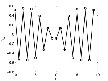
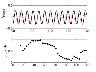
Figure 9: Left: The driven chain at $t\approx 110$ (markers) and an exact dark breather (solid line) for $\omega_{b}=1.99$. Top Right: Evolution of the middle bead for the driven chain (dashed line) and exact dark breather (solid line). Bottom Right: The $l^{\infty}$ norm of the difference between the driven chain and exact dark breather for time points such that $y_{\mathrm{middle}}(t)$ is at a maximum.

The timescale which is required for the dark breathers to manifest via the actuation is crucial, as the physical system will have dissipative effects, which may be detrimental to the emergence of the dark breathers. Dissipation can be modeled Nature11 by modifying Eq. (1) as

$$M\ddot{u}_{n}=A[\delta_{0}+u_{n-1}-u_{n}]_{+}^{3/2}-A[\delta_{0}+u_{n}-u_{n+1}]_{+}^{3/2}-\frac{M}{\tau}\dot{u}_{n}.$$ (15)

For small values of the dissipation coefficient (i.e. for large $\tau$), dark breathers can still emerge (see Fig. 10 left), however for larger values, the dissipative effects are indeed detrimental to the emergence of the dark breathers (see Fig. 10 right). Thus, it is important to consider physical values of the parameters. The scaling,

$$u_{n}=\delta_{0}\,\tilde{u}_{n},\quad\quad t=\beta\,\tilde{t},\quad\quad\tau=\beta\,\tilde{\tau},\quad\beta=\sqrt{\frac{2M}{3A\delta_{0}^{1/2}}},$$

can be used to recover the physically relevant solutions, where the variables with the tilde represent solutions in the idealized case of $\delta_{0}=M=1$ and $A=2/3$ used above. For a chain of 316-stainless steel beads we have,

$$A=\frac{E\sqrt{2R}}{3(1-\nu^{2})},\quad\quad M=4\pi R^{3}\rho/3,\,\quad\quad\delta_{0}=(F_{0}/A)^{2/3},$$

where $E=193\cdot 10^{9}$  $(N/m^{2})$ is the Young’s Modulus, $R=9.525\cdot 10^{-3}\,(m)$ is the bead radius, $\nu=0.3$ is the Poisson Ratio, $\rho=8027.17$  $(kg/m^{3}$) is the bead density, and $F_{0}=20\,(N)$ is a typical precompression force which results in physical parameter values of $A\approx 9.7576\cdot 10^{9}\,(N/m^{3/2})$, $M\approx 0.0029\,(kg)$ and $\delta_{0}\approx 1.6136\cdot 10^{-6}\,(m)$. The scaling parameter in this case becomes $\beta\approx 3.9533\cdot 10^{-5}$. Thus, a breather appearing at approximately $\tilde{t}\approx 90$ would correspond to $t=90\beta\approx 3.6\,(ms)$ in physical time. The tested dissipation coefficients of $\tilde{\tau}=100$ and $\tilde{\tau}=10$ would become $\tau=100\beta\approx 4\,(ms)$ and $\tau=10\beta\approx 0.4\,(ms)$ respectively in the physical scaling. Thus, if one were able to carry out experiments where the dissipation constant is on the order of $\tau=4\,(ms)$, dark breathers should be detectable. We note that the experimentally relevant dissipation constant in Ref. Nature11 corresponds to $\tau=2\,(ms)$, which demonstrates the feasibility of detecting dark breathers in currently available experimental settings of granular chains.

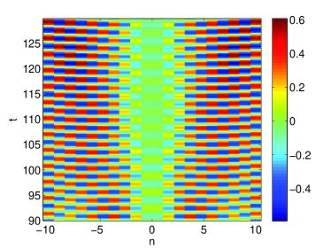
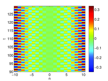
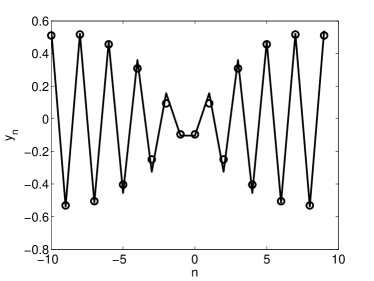
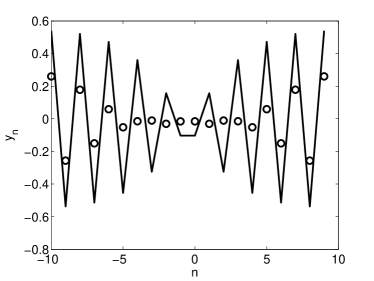
Figure 10: Top: Contour plots of the space-time evolution of the driven chain with the same parameters as in Fig. 8 and with a dissipation coefficient of $\tau=100$ (left) and $\tau=10$ (right). Bottom: Comparison between the driven chain (markers) and exact breather solution (solid line) for $\tau=100$ (left) and $\tau=10$ (right). Here the times were chosen to yield the closest resemblance.

XI Discussion and future directions

We have demonstrated that dark breathers are not only an interesting entity of the granular crystal model from a theoretical point of view, but are also within the reach of currently available experimental technology, given the ability to actuate both ends of the chain of beads. On the theoretical side, a useful qualitative (although only approximate) approach towards the understanding of such states arises through the use of the NLS reduction. On the other hand, their detailed numerical study illustrates the existence of a small amplitude branch arising from one of the linear eigenmodes of the system, but also of a large amplitude branch which cannot be captured from our analytical considerations. The destructive interference of the signals (at the appropriate frequency inside the pass band) induced by the two actuators produces a waveform proximal to the exact dark breathers, and this observation is found to persist even in the presence of realistic values of the dissipation within the system.

Besides the realization of such experiments which would be of particular value, our study also raises several interesting open problems from the mathematical/theoretical point of view. Among these, we highlight a band analysis of the Floquet multipliers in order to capture the continuous spectrum of the infinite lattice problem; also, a proof of the numerically observed nonlinear instability, apparently present due to a non-trivial scale invariance that we identified; finally, the rigorous justification of the NLS equation for dark breathers and especially of its regime of validity (which in our case appears to be relatively limited at least in a quantitative sense).

The readiness of the solutions to move, via random perturbations of the unstable solutions, and the apparent spatial translation invariance of the system render also plausible the potential existence of traveling breathers. In that light, a computational study of such states along the lines of earlier similar studies in the realm of the discrete NLS equation floria ; our1 ; hadi would be of particular interest. The potential emergence of dark breathers in inhomogeneous chains, such as dimers Boechler2009 ; Theo2010 or trimers apl11 may be another issue to computationally consider in detail, since bright breathers have been identified as relatively robust nonlinear states in such settings Boechler2009 ; Theo2010 ; hooge11 .

Such studies are currently in progress and will be reported in future publications.

References

- (1) J.M. English and R.L. Pego, Proceedings of the AMS 133, 1763 (2005)
- (2) A. Stefanov and P.G. Kevrekidis, J. Nonlin. Sci. 22, 327 (2012).
- (3) V. F. Nesterenko, Dynamics of Heterogeneous Materials (Springer-Verlag, New York, NY, 2001).
- (4) S. Sen, J. Hong, J. Bang, E. Avalos, and R. Doney, Phys. Rep. 462, 21 (2008).
- (5) C. Daraio, V. F. Nesterenko, E. B. Herbold, and S. Jin, Phys. Rev. E. 73, 026610 (2006).
- (6) C. Coste, E. Falcon, and S. Fauve, Phys. Rev. E. 56, 6104 (1997)
- (7) C. Daraio, V. F. Nesterenko, E. B. Herbold, and S. Jin, Phys. Rev. Lett. 96, 058002 (2006).
- (8) J. Hong, Phys. Rev. Lett. 94, 108001 (2005).
- (9) F. Fraternali, M. A. Porter, and C. Daraio, Mech. Adv. Mat. Struct. 17(1), 1 (2010).
- (10) R. Doney and S. Sen, Phys. Rev. Lett. 97, 155502 (2006).
- (11) D. Khatri, C. Daraio, and P. Rizzo, SPIE 6934, 69340U (2008).
- (12) A. Spadoni and C. Daraio, Proc Natl Acad Sci USA, 107, 7230, (2010).
- (13) See e.g. B. Liang, B. Yuan and J.-c. Cheng, Phys. Rev. Lett. 103, 104301 (2009) and also X.F. Li, X. Ni, L. Feng, M.-H. Lu, C. He and Y.-F. Chen, Phys. Rev. Lett. 106, 084301 (2011).
- (14) N. Boechler, G. Theocharis, C. Daraio, Nature Materials 10, 665 (2011).
- (15) C. Daraio, V. F. Nesterenko, E. B. Herbold, and S. Jin, Phys. Rev. E 72, 016603 (2005).
- (16) V. F. Nesterenko, C. Daraio, E. B. Herbold, and S. Jin, Phys. Rev. Lett. 95, 158702 (2005).
- (17) S. Flach and A. V. Gorbach, Phys. Rep. 467, 1 (2008).
- (18) G. Theocharis, M. Kavousanakis, P. G. Kevrekidis, C. Daraio, M. A. Porter, and I. G. Kevrekidis, Phys. Rev. E 80, 066601 (2009).
- (19) G. Theocharis, N. Boechler, P. G. Kevrekidis, S. Job, M. A. Porter, and C. Daraio, Phys. Rev. E 82, 056604 (2010).
- (20) N. Boechler, G. Theocharis, S. Job, P. G. Kevrekidis, M. A. Porter and C. Daraio, Phys. Rev. Lett. 104, 244302 (2010).
- (21) C. Hoogeboom, P. G. Kevrekidis, arXiv:1105.6354.
- (22) G. James, C.R. Acad. Sci.,Ser.1:Math 332, 581 (2001).
- (23) G. James, J. Nonlinear Sci. 13, 27 (2003).
- (24) G. Schneider, Appl. Anal. 89 1523 (2010).
- (25) M. Chirilus-Bruckner, C. Chong, O. Prill and G. Schneider, Disc. Cont. Dyn. Sys. S 5, 879-901 (2012).
- (26) B. Sanchez-Rey, G. James, J. Cuevas, and J. F. R. Archilla, Phys. Rev. B 70, 014301 (2004).
- (27) G. Huang and B. Hu, Phys. Rev. B 57, 5746 (1998).
- (28) Y.S. Kivshar and X. Yang, Phys. Rev. E 49, 1657 (1994).
- (29) D.E. Pelinovsky, Localization in Periodic Potentials: From Schrödinger Operators to the Gross-Pitaevskii Equation (Cambridge University Press, Cambridge, 2011).
- (30) S. Aubry, Physica D 216, 1 (2006).
- (31) Chaos, S. Flach and A. V. Gorbach 15 015112 (2005).
- (32) J. Gómez-Gardenes, F. Falo, L.M. Floría, Phys. Lett. A 332, 213 (2004).
- (33) T. R. O. Melvin, A. R. Champneys, P. G. Kevrekidis, J. Cuevas, Phys. Rev. Lett. 97 124101 (2006); see also Phys. D 237, 551 (2008).
- (34) M. Syafwan, H. Susanto, S.M. Cox and B.A. Malomed, J. Phys. A 45, 075207 (2012).
- (35) N. Boechler, J. Yang, G. Theocharis, P.G. Kevrekidis and C. Daraio, J. Appl. Phys 109, 074906 (2011).