Graphene flakes with defective edge terminations: Universal and topological aspects, and one-dimensional quantum behavior

Abstract

Systematic tight-binding investigations of the electronic spectra (as a function of the magnetic field) are presented for trigonal graphene nanoflakes with reconstructed zigzag edges, where a succession of pentagons and heptagons, that is 5-7 defects, replaces the hexagons at the zigzag edge. For nanoflakes with such reczag defective edges, emphasis is placed on topological aspects and connections underlying the patterns dominating these spectra. The electronic spectra of trigonal graphene nanoflakes with reczag edge terminations exhibit certain unique features, in addition to those that are well known to appear for graphene dots with zigzag edge termination. These unique features include breaking of the particle-hole symmetry, and they are associated with nonlinear dispersion of the energy as a function of momentum, which may be interpreted as nonrelativistic behavior. The general topological features shared with the zigzag flakes include the appearance of energy gaps at zero and low magnetic fields due to finite size, the formation of relativistic Landau levels at high magnetic fields, and the presence between the Landau levels of edge states (the socalled Halperin states) associated with the integer quantum Hall effect. Topological regimes, unique to the reczag nanoflakes, appear within a stripe of negative energies $\varepsilon_{b}<\varepsilon<0$, and along a separate feature forming a constant-energy line outside this stripe. The $\varepsilon_{b}$ lower bound specifying the energy stripe is independent of size.

Prominent among the patterns within the $\varepsilon_{b}<\varepsilon<0$ energy stripe is the formation of three-member braid bands, similar to those present in the spectra of narrow graphene nanorings; they are associated with Aharonov-Bohm-type oscillations, i.e., the reczag edges along the three sides of the triangle behave like a nanoring (with the corners acting as scatterers) enclosing the magnetic flux through the entire area of the graphene flake. Another prominent feature within the $\varepsilon_{b}<\varepsilon<0$ energy stripe is a subregion of Halperin-type edge states of enhanced density immediately below the zero-Landau level. Furthermore, there are features resulting from localization of the Dirac quasiparticles at the corners of the polygonal flake.

A main finding concerns the limited applicability of the continuous Dirac-Weyl equation, since the latter does not reproduce the special reczag features. Due to this discrepancy between the tight-binding and continuum descriptions, one is led to the conclusion that the linearized Dirac-Weyl equation fails to capture essential nonlinear physics resulting from the introduction of a multiple topological defect in the honeycomb graphene lattice.

I Introduction

I.1 Edge terminations and their nanoelectronics potential

Graphene is a single-layer honeycomb lattice of carbon atoms and exhibits novel behavior due to the relativistic-like character of quasiparticle (particle-hole) excitations near the Fermi level (the Dirac neutrality point).geim04 ; geim05 In addition to the intrinsic interest in this material, the potential of graphene for nanoelectronics applications has generated considerable amount of research regarding the physics governing the Dirac electrons in graphene nanostructures. Initially graphene nanoribbons attracted most of the attention; see, e.g., Refs. dres96, ; waka99, ; cai10, . However, in the last couple of years the focus is being shifted to studying zero-dimensional stuctures like graphene quantum dots and graphene quantum voids (see, e.g., Refs. wuns08, ; roma09, ; wurm09, ; libi09, ; zhan08, ; pala07, ; ezaw08, ; pota10, ; yan10, ; yann10, ; roma11, ), as well as graphene nanorings (see, e.g., Refs. rech07, ; baha09, ; roma12, ).

In addition to the novelty of the relativistic nature of the trapped quasiparticles, the honeycomb lattice of graphene provides for a variety of edge terminations (see below), which have no parallel in the case of semiconductor nanosystems. More importantly, it is now understood dres11 that the electronic properties of graphene nanostructures are drastically influenced by the character of the edge termination.

The physical graphene edges develop along the crystallographic axes of the honeycomb lattice, and they may exhibit two distinct types of terminations: zigzag or armchair. One-type edges may intersect at angles of $60^{\circ}$ or $120^{\circ}$, yielding graphene flakes and voids with regular trigonal or hexagonal shapes. Square graphene dots can also be envisioned, but they have edges of a mixed zigzag and armchair character. Ring-like trigonal, hexagonal, and square-like graphene structures are also the focus of intensive theoretical studies.

The theoretical advances regarding the properties of graphene edges have in turn motivated considerable experimental efforts aiming at producing graphene edges with a high-degree of purity with respect to the edge termination (zigzag or armchair), and remarkable successes have been already reported; see, e.g., Refs. dres11, ; jia09, ; krau10, ; neme10, ; yang10, ; shi11, ; lu11, ; begl11, .

While the zigzag and armchair edges were known for some time from the theoretical studies on graphene nanoribbons, the recent consideration (anticipated theoretically and confirmed through observation) of yet another physical edge, formed through reconstruction of the zigzag edge, has added a new dimension to the research on the electronic properties of graphene nanostructures.kosk08 ; kosk09 ; rodr11 ; osta11 Indeed, this reconstructed edge, which is usually called reczag and consists of a succession of pentagons and heptagons (5$-$7 defect) according to the Stone-Wales-defects prescription, has the potential to yield new distinctive features in the electronic structure of graphene nanostructures, whether these nanostructures are graphene flakes, voids, or graphene rings. The reczag edge belongs to a general class of defective formations in graphene: a related defective formation is the alternation of pentagons and octagons (5$-$8$-$5 defect), which has also been observed experimentally in the last couple of years and which is expected to behave like a “quantum wire” within the graphene sheet. dres11 ; lahi10

I.2 Topological aspects: Coexistence of quantum-wire, ideal-ring, and quantum-dot singly-connected-geometry behavior

Experimentally, two-dimensional semiconductor quantum dots (SQDs) exhibit usually soft edges, west96 ; west98 which can be modeled by a harmonic potential confinement. kouw01 ; reim02 ; yann07 Nevertheless important theoretical studies concerning topological aspects of nonrelativistic electrons in finite systems under strong magnetic fields have been performed by assuming hard-wall boundaries. Well known among such studies are the investigations halp82 ; stre84 ; stre87 ; hout89 ; mont08 ; mont11 (initiated by Halperin halp82 ) regarding the edge states related to the integer-quantum-Hall-effect (IQHE) and those imry88 ; imry89 ; avis93 ; tana98 (initiated by Sivan and Imry imry88 ) on the Aharonov-Bohm (AB) oscillations which are superimposed on the de Haas - van Alphen (dHvA) oscillations. Halperin introduced a hard boundary through an infinite-box-type confining potential, while Sivan and Imry used a 10 $\times$ 10 square-lattice tight-binding (TB) model.

Finite graphene nanosystems [Graphene QDs (GQDs) or nanoflakes] offer a broader framework to study such topological connections. Most importantly, original trends and phenomena can emerge dres96 ; yann10 ; roma11 which have no analog with the physics of semiconductor QDs. Indeed, compared to SQDs, Graphene QDs exhibit distinct features such as: 1) They possess yann10 ; roma11 ; andr12 atomically defined sharp physical boundaries (because of the abrupt termination of the honeycomb lattice). 2) Due to the underlying honeycomb lattice of graphene, the confined electrons are most appropriately described by TB modeling,dres96 ; zhan08 ; roma11 ; geim09 , while at the same time the corresponding continuous description reveals that they behave as massless relativistic particles obeying the Dirac-Weyl (DW) equation. roma11 ; geim09 ; aban06 ; brey06.2 3) The natural shapes of GQDs are not circular, but triangular, hexagonal, or rhombus-like; roma11 as a result, the electronic spectra can explore geometric symmetries lower than the circular one.roma12 4) As we will show below, the presence of defective edges introduces a quantum-wire and/or ring-type (doubly-connected-geometry) behavior, in addition to the singly-connected QD behavior familiar from the theoryimry89 of SQDs with sharp edges.

Figure 1: (Color online) Distribution of the hopping matrix elements $t_{k}$ (see Table 1) for the reczag edge.

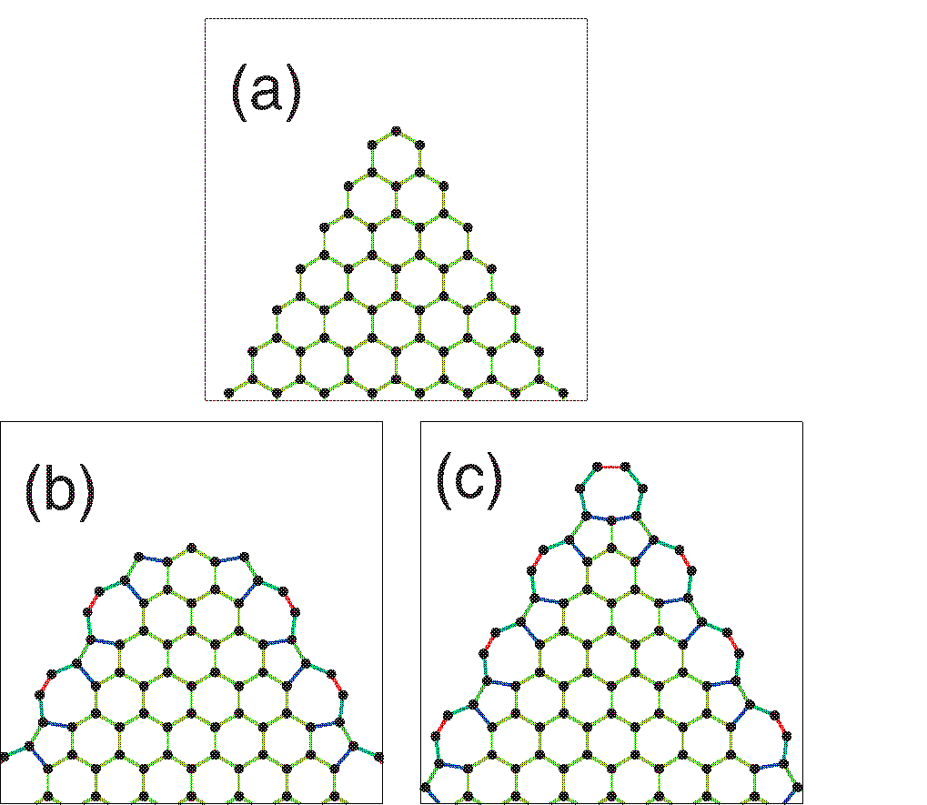
Figure 2: (Color online) Diagrams of corners used for the equilateral trigonal graphene flakes. (a) corner for zigzag edges. (b) Type-I corner for reczag edges. (c) Type-II corner for reczag edges.

I.3 Main findings

The main findings of the paper are:

(I) Beyond the well known features found for graphene quantum dots with zigzag edge terminations, the electronic spectra (as a function of the magnetic field $B$) of trigonal graphene nanoflakes with reconstructed edges (that is, edge termination with 5-7 defects; see Fig. 1 and Fig. 2) exhibit unique additional regimes; they break the particle-hole symmetry and are characterized by a nonlinear dispersion of the electron energy versus momentum, associated with a nonrelativistic quantum mechanical description.

(II) The general features shared by graphene flakes with reczag termination with those having zigzag edges, include the appearance of energy gaps at zero and low magnetic fields due to the finite size (designated as region A, see Fig. 3), the formation of relativistic Landau levels (labeled as regions B, see Fig. 3) at high magnetic fields, and the presence between the Landau levels of edge states (socalled Halperin states, labeled as regions $C_{i}$, see Fig. 3) associated with the IQHE. The characteristic length-scalemont10 for the Halperin-type edge states is the cyclotron radius (magnetic length $l_{B}$) of the electron orbit (inversely proportional to the strength of the applied magnetic field).

(III) The unique regimes that emerge in the spectrum of GQDs with reczag (reconstructed zigzag) edges include: (a) several features within a band of negative energies $\varepsilon_{b}=-0.205t<\varepsilon<0$ [region labeled as D below in Fig. 3(c); divisible in regions D1 and D2, see Fig. 4], and (b) a feature forming a constant-energy line at $\varepsilon_{c}\approx-0.297t$ [region labeled as E1, see Fig. 3(c)]. The $\varepsilon_{b}$ lower bound of the region D [see (a) above] is independent of size.

(IV) Prominent among the features within the aforementioned $\varepsilon_{b}=-0.205t<\varepsilon<0$ energy stripe is the formation of three-member braid bands (subregion D1, see Fig. 4), similar to those presentbaha09 ; roma12 in the spectra of narrow graphene nanorings, which were shown to be associated with Aharonov-Bohm oscillations in graphene nanosystems.roma12 This suggests that the reczag edge behaves in a manner that is analogous to a nanoring enclosing the magnetic flux $\Phi$ through the entire area of the graphene flake; $\Phi$ will be given in units of $\Phi_{0}=hc/e$. Obviously the length scale governing the behavior of these edge states associated with the reczag defective edge is the characteristic length ${\cal L}$ of the entire graphene flake. This analogy is further substantiated with an analysis using a simple nonrelativistic 1D superlattice model (see Sec. III.2.2) where the corners of the trigonal flake are modeled by appropriate scatterers.

(V) Another prominent feature within the $\varepsilon_{b}=-0.205t<\varepsilon<0$ energy stripe is a subregion (D2) of Halperin-type edge states with enhanced density below the zero-Landau level; see Fig. 4 and Sec. III.2.3.

(VI) Furthermore, there are features resulting from localization of the Dirac quasiparticles at the corners of the polygonal flake (regions labeled as E1 and E2, see Sec. III.2.4).

(VII) A main finding concerns the limited applicability of the continuous Dirac-Weyl equation. As we explicitly show in Sec. IV, the general features, e.g., the relativistic Landau levels, and the Halperin-type edge states, are also present in the continuum-DW reczag spectra. However, concerning the unique features found via TB calculations, only the feature of the Halperin-type edge states with an enhanced density spectrum (D2 region) maintains also in the continuum spectra; the rest of the special reczag features [see (III), (IV), and (VI) above] are missing in the continuum- DW spectrum. Due to this major discrepancy between the TB and continuum descriptions, we are led to conclude that the linearized DW equation fails to capture essential nonlinear physics (i.e., a nonlinear dispersion of energy versus momentumnote3 coexisting with the Dirac cone), resulting from the introduction of a nontrivial (multiple) topological defectvozm07 ; bern08 ; vozm10 ; mesa09 ; note4 (e.g., reconstructed reczag edge) in the honeycomb graphene lattice.

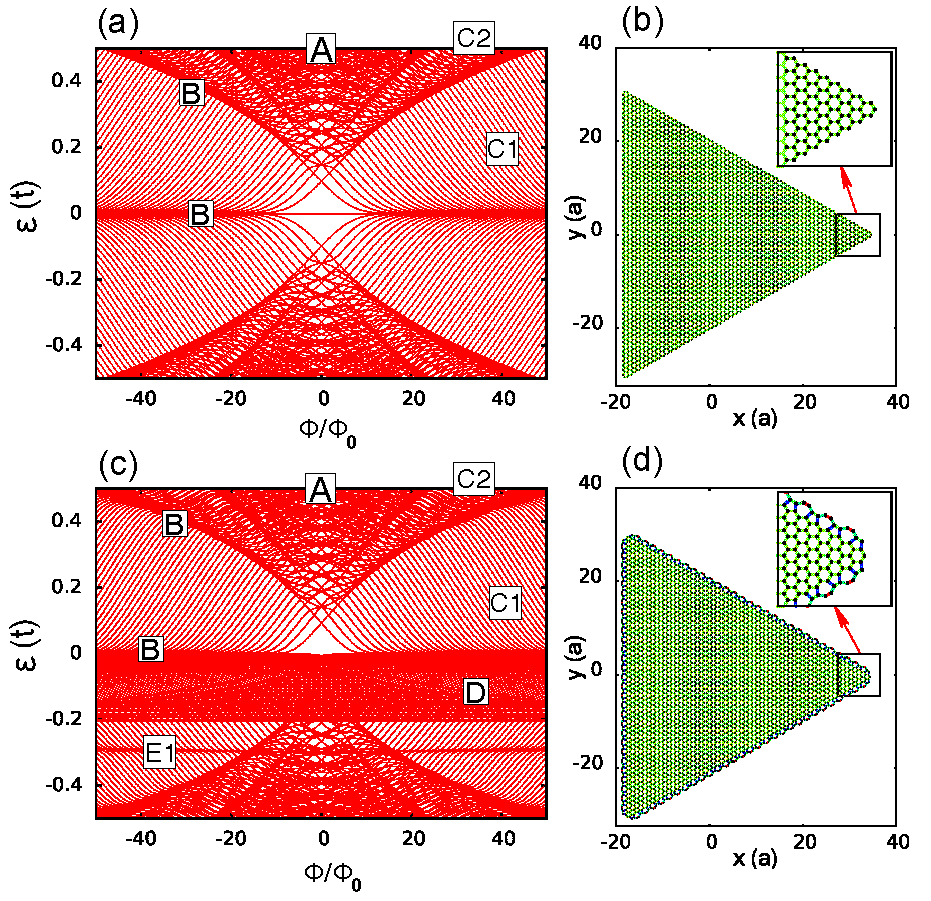
Figure 3: (Color online) (a) TB single-particle spectrum for a zigzag trigonal graphene dot as a function of the magnetic field (the magnetic flux $\Phi$ over the whole dot). (b) Shape of the corresponding equilateral trigonal graphene dot with zigzag edges; it has 61 hexagons in the outer row along each side (the total number of carbon atoms is 3966). (c) TB single-particle spectrum for a type-I reczag trigonal graphene dot as a function of the magnetic field (the magnetic flux $\Phi$ over the whole dot). (d) Shape of the corresponding trigonal graphene dot with reczag edges (type-I corner); it has 60 hexagons in the outer unreconstructed row along each side (the total number of carbon atoms is 4731). Energy in units of the tight-binding hopping-parameter $t=2.7$ eV. Lengths in units of the honeycomb graphene lattice constant $a=0.246$ nm. The magnetic flux is given in units of $\Phi_{0}=hc/e$.

I.4 Plan of paper

In addition to this section, the Introduction consisted of three other ones: The first (Sec. I.1) provided background information concerning the different graphene edge terminations and their nanoelectronics potential, while the second (Sec. I.2) introduced the topological aspects. The main findings of this paper were outlined in Sec. I.3.

The remaining of the paper is organized as follows:

Sec. II recapitulates briefly the tight-binding and continuum Dirac-Weyl methodologies.

Our main results from the tight-binding calculations are presented in Sec. III. This section is further divided in two parts: Sec. III.1 describes the general features of the spectra of trigonal flakes which are shared with GQDs having other edge terminations (e.g., zigzag or armchair). The special features which are unique to the reczag edge termination are presented in Sec. III.2. For a synopsis of these general and special features, see the section describing the main findings (Sec. I.3). Three different sizes of trigonal graphene flakes are considered in Sec. III, with the two smaller sizes being discussed in Sec. III.3.

The corresponding continuous Dirac-Weyl description for a circular reczag GQD is elaborated and contrasted to the TB results in Sec. IV.

A summary and discussion of our results is given in Sec. V.

Finally the Appendix presents the explicit expressions for the transfer matrices employed in Sec. III.2.2.

II Methodology

In previous publications, we studied primarily graphene quantum dots and graphene nanorings with zigzag edge terminations. In this paper, we carry out systematic investigations of the electronic properties of graphene flakes with reczag edge terminations and the shape of a regular triangle (see Fig. 1 and Fig. 2), and for the cases of zero-magnetic, low-magnetic, and high-magnetic fields. In particular, we study the excitation spectra using independent-particle treatments, i.e., we use both the tight-binding approach and the semianalytic continuum Dirac-Weyl equations; see, e.g., Refs. roma11, ; roma12, .

II.0.1 Basic elements of TB approach

To determine the single-particle spectrum [the energy levels $\varepsilon_{i}(B)$] in the tight-binding calculations for the graphene nanoflakes, we use the hamiltonian

$$H_{\text{TB}}=-\sum_{<i,j>}\tilde{t}_{ij}c^{\dagger}_{i}c_{j}+h.c.,$$ (1)

with $<>$ indicating summation over the nearest-neighbor sites $i,j$. The hopping matrix element

$$\tilde{t}_{ij}=t_{ij}\exp\left(\frac{ie}{\hbar c}\int_{{\bf r}_{i}}^{{\bf r}_{j}}d{\bf s}\cdot{\bf A}({\bf r})\right),$$ (2)

where ${\bf r}_{i}$ and ${\bf r}_{j}$ are the positions of the carbon atoms $i$ and $j$, respectively, and ${\bf A}$ is the vector potential associated with the applied perpendicular magnetic field $B$. In the case of a zigzag edge termination, $t_{ij}=t=2.7$ eV. In the case of the reconstructed reczag edge, four additional values (see Fig. 1) for the hopping matrix elements must be considered for carbon pairs participating in the defective edge.kosk08 ; osta11 These values are listed in Table 1.

Table 1: DFT extracted values for the hopping matrix elements $t_{k}$ (see Fig. 1) in the TB modeling of a reczag edge, according to Ref. kosk08, .

$t_{1}/t$	$t_{2}/t$	$t_{3}/t$	$t_{4}/t$
0.91	0.99	0.97	1.5

The diagonalization of the TB hamiltonian [Eq. (1)] is implemented with the use of the sparse-matrix solver ARPACK.arpack We note here that, unlike the continuous Dirac-Weyl equations,rech07 ; roma11 both the $K$ and $K^{\prime}$ valleys are automatically incorporated in the tight-binding treatment of graphene sheets and nanostructures.

II.0.2 Basic elements of continuous Dirac-Weyl equations

In polar coordinates, the low-energy noninteracting graphene electrons (around a given $K$ or $K^{\prime}$ point) are most often described via the continuous DW equation.geim09 Circular symmetry leads to conservation of the total pseudospingeim09 $\hat{\jmath}=\hat{m}+\hat{\sigma}_{z}$, where $\hat{m}$ is the angular momentum and $\hat{\sigma}_{z}$ the spin of a Dirac electron. The reczag edge does not couple the two valleys,osta11 and as a result, we seek solutions for the two components $\Psi_{A}({\bf r})$ and $\Psi_{B}({\bf r})$ or $\Psi^{\prime}_{A}({\bf r})$ and $\Psi^{\prime}_{B}({\bf r})$ of the single-particle electron orbital (a spinor). The indices $A$ and $B$ denote the two graphene sublattices and the unprimed and primed symbols are associated with the $K$ and $K^{\prime}$ valleys.

Below we focus on the $K$ valley; similar equations apply also to the $K^{\prime}$ valley. In polar coordinates, one has:

$$\psi_{m}({\bf r})=\left(\begin{array}[]{c}\Psi_{A}({\bf r})\\ \Psi_{B}({\bf r})\end{array}\right)=\left(\begin{array}[]{c}e^{im\theta}\chi_{A}(r)\\ ie^{i(m+1)\theta}\chi_{B}(r)\end{array}\right).$$ (3)

The angular momentum $m$ takes integer values; for simplicity in Eq. (3) and in the following, the subscript $m$ is omitted in the sublattice components $\Psi_{A}$, $\Psi_{B}$ and $\chi_{A}$, $\chi_{B}$.

With Eq. (3) and a constant magnetic field $B$ (symmetric gauge), the DW equation reduces (for the $K$ valley) to

$$\frac{d}{dx}\chi_{B}+\frac{1}{x}\left(m+1+\frac{x^{2}}{2}\right)\chi_{B} = \varepsilon\chi^{A}$$

$$\frac{d}{dx}\chi_{A}-\frac{1}{x}\left(m+\frac{x^{2}}{2}\right)\chi_{A} = -\varepsilon\chi_{B};$$ (4)

where the reduced radial coordinate $x=r/l_{B}$ with $l_{B}=\sqrt{\hbar c/(eB)}$ the magnetic length. The reduced single-particle eigenenergies $\varepsilon=E/(\hbar v_{F}/l_{B})$, with $v_{F}$ the Fermi velocity.

The solutions of the DW equations for both valleys in the case of a circular GQD with a reczag edge is presented in detail in Sec. IV.

III Tight-binding description for reczag trigonal flakes

III.1 General features

An example for a trigonal quantum flake is given in Fig. 3 where the single-particle spectrum (as a function of the magnetic field) of a dot with reczag edges (and type-I corners; see Fig. 2) is compared to that of a dot of similar size, but with unreconstructed zigzag edges. Various aspects of trigonal GQDs with pure zigzag edges have been studied earlier; pala07 ; pota10 ; ezaw10 however, for completeness and to allow ready comparisons to be made, we display and briefly comment on the corresponding spectrum [see Fig. 3(a)]. In particular, we have marked main features (or regimes) of the zigzag spectrum as follows: The regime of zero and low-magnetic fields is denoted by “A”; it exhibits energy gaps due to finite-size effects. The regime of Landau levels (LLs) formed at high magnetic fields is denoted by “B” (only the $n=0$ and $n=-1$ levels are denoted). The “C_i’s” denote the edge states yann10 ; roma11 which connect the $|i-1|\text{-}th$ and $|i|\text{-}th$ LLs. The general regimes A, B, and C are also present in the spectra of trigonal flakes with reczag edges, as an inspection of Fig. 3(c)] readily reveals.

We note that the three regimes A, B, and C_i have corresponding analogs in the case of a QD with nonrelativistic electrons confined by a hard-wall boundary.imry88 ; imry89 ; avis93 ; tana98 These analogies exist despite the well-known differences arising from the relativistic nature of Dirac electrons, e.g., the energies of the Landau levels in graphene are $E_{n}=\operatorname{sgn}(n)v_{F}\sqrt{2e\hbar B|n|}$, $n=0,\pm 1,\pm 2,\ldots$, (square-root $B$-dependence) compared to $E_{n}=\hbar\omega_{c}(n+1/2)$, $n=0,1,2,\ldots$, [with $\hbar\omega_{c}=eB/(m^{*}c)$, linear dependence on $B$] for the case of a nonrelativistic 2D electron gas. Such analogs emerge from underlying universal and topological properties of the 2D finite systems under high magnetic fields, i.e., when $l_{B}\equiv\sqrt{\hbar c/(eB)}<{\cal L}$ with ${\cal L}$ being a characteristic length of the nanosystem. Naturally, the energy of the LLs depends on the cyclotron orbit alone, and thus it is independent of the size and shape of the dot. But also, this size-and-shape independence is shared to a large degreenote1 by the Halperin-type edge states between LLs,halp82 whose energy can be derived (to the lowest order) from a semiclassical or WKB quantization of a single arc of the skipping orbits, both for nonrelativistic hout89 ; mont08 ; mont11 and Dirac electrons.mont10

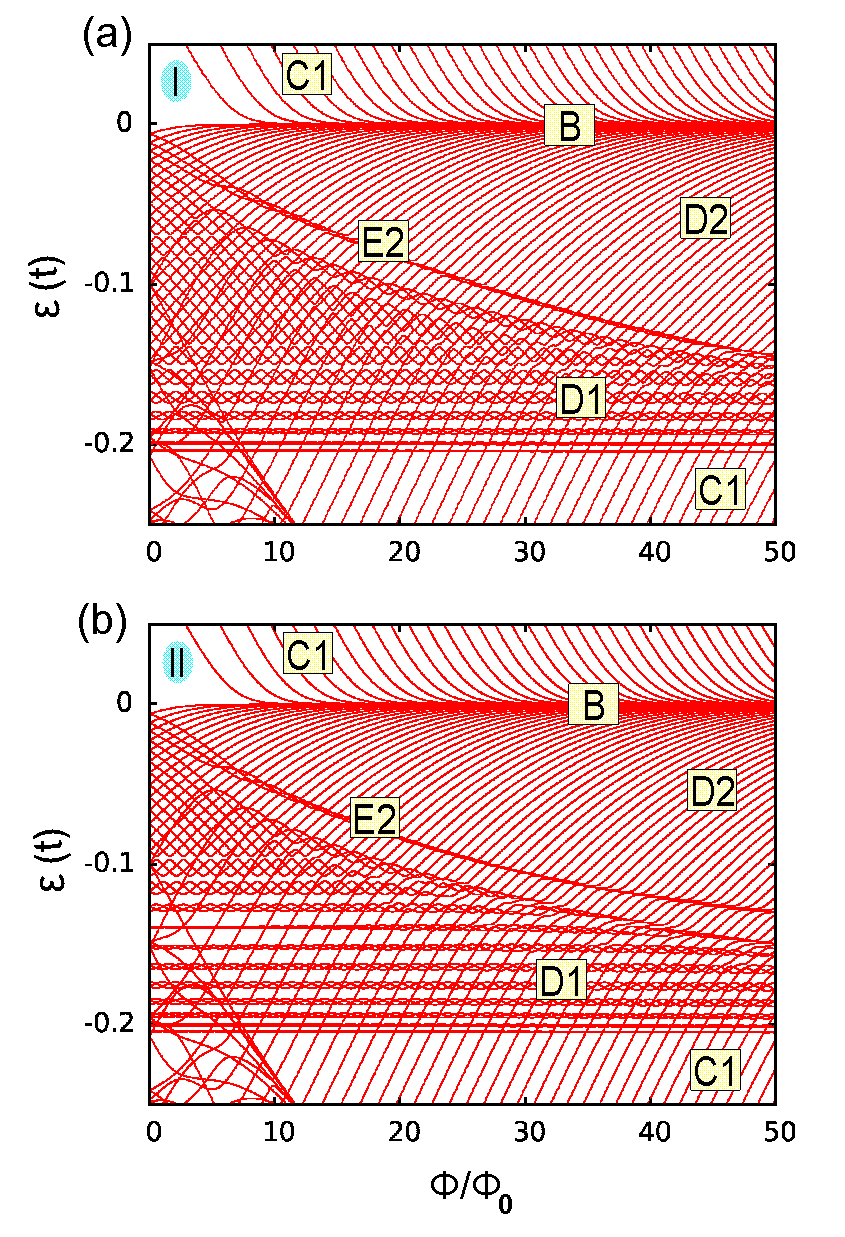
Figure 4: (Color online) (a) An enlarged section of the regime marked as D in Fig. 3(c), showing the TB single-particle spectrum for a reczag trigonal graphene dot (with type-I corners), as a function of the magnetic field (the magnetic flux $\Phi$ over the whole dot). (b) The TB spectrum for the corresponding reczag trigonal GQD with type-II corners. Energy in units of the tight-binding hopping-parameter $t$. The magnetic flux is given in units of $\Phi_{0}=hc/e$.

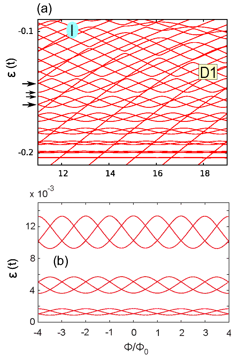
Figure 5: (Color online) An enlarged section of the regime marked as D1 in Fig. 4(a) showing the TB single-particle spectrum for a reczag trigonal graphene dot (with type-I corners), as a function of the magnetic field (the magnetic flux $\Phi$ over the whole dot). The horizontal arrows highlight the alternation 2-1-1-2 (1-2-2-1) in the state degeneracy between two successive braid bands at $\Phi/\Phi_{0}=n$ ($\Phi/\Phi_{0}=n+1/2$), $n=0,1,2,\ldots$. (b) An example (for reasons of comparison) of a TB single-particle spectrum for a narrow trigonal graphene ring with zigzag edge terminations. Such nanorings were used in Ref. roma12, to study the Aharonov-Bohm oscillatory patterns in graphene nanosystems.

Of interest for the present study are the Aharonov-Bohm-type refinements concerning the Halperin-type edge states investigatedimry88 ; imry89 ; avis93 ; tana98 for the case of SQDs. Indeed, Refs. imry88, and imry89, argued that, in the case of the finite, singly-connected QDs, the Halperin-type edge states form an effective ring; in a semiclassical picture they correspond to grazing orbits (see also Ref. blasc97, ), reminiscent of the whispering gallery trajectoriesboga72 investigated at low magnetic fields. As a result the associated spectra must exhibit a dependence on the total magnetic flux through the area of the QD, which leads to the emergence of AB-type oscillations in the total Landau magnetization of the dot. Specifically these high-$B$ AB oscillations are superimposed on the much larger de Haas - van Alphen ones, and they tend to decrease as $B$ increases.

It is apparent, that similar high-$B$ AB-type effects are also present in the case of GQDs with zigzag and reczag terminations: for example, for the GQDs associated with Figs. 3(a) and 3(c), it suffices to calculate the Landau magnetization assuming a zero-temperature canonical ensemble and a number, $N$, of Dirac electrons large enough so that the corresponding Fermi level $\varepsilon_{F}>0.2t$.

We stress that our findings regarding trigonal flakes with reczag edges go beyond (see III.2) the general features described above. Indeed, one of our main findings is that trigonal flakes support, in addition to the high-$B$, singly-connected-dot AB behavior, oscillatory behavior similar to the low-$B$ Aharonov-Bohm effect, familiar from semiconductorimry83 ; loss91 ; glaz09 ; imry09 and graphene nanorings.rech07 ; roma12 The coexistence, in the same nanostructure, of these two distinct AB behaviors (associated with singly-connected and doubly-connected geometries) has no analog in previously considered nanosystems, and it is a special feature unique to graphene defective edges.

III.2 Unique features due to the reczag edge

Having discussed the common general features shared by both the zigzag and reczag trigonal graphene flakes (see Sect. III.1), we turn now to study the unique features emerging solely in the case of reczag trigonal flakes. An inspection of the electronic spectra in Figs. 3(a) and 3(c) shows that the main differences arise from the presence of the two regimes denoted as D and E1 in the case of the reczag dot. In particular, the regime D consists of the features within a band of negative energies $\varepsilon_{b}=-0.205t<\varepsilon<0$, while the regime E1 consists of a constant-energy line at $\varepsilon_{c}\approx-0.297t$. (The reconstructed reczag edge violates particle-hole symmetry, while as is well known the zigzag edge preserves it.) We found that the lower energy bound $\varepsilon_{b}$ of the D regime is independent of the size and shape (e.g., hexagonal versus trigonal flake), as well as of the type of corners (type-I versus type-II, see Fig. 2); $\varepsilon_{b}$ depends only on the values of the TB hopping matrix elements $t_{k}$ (see Table 1).

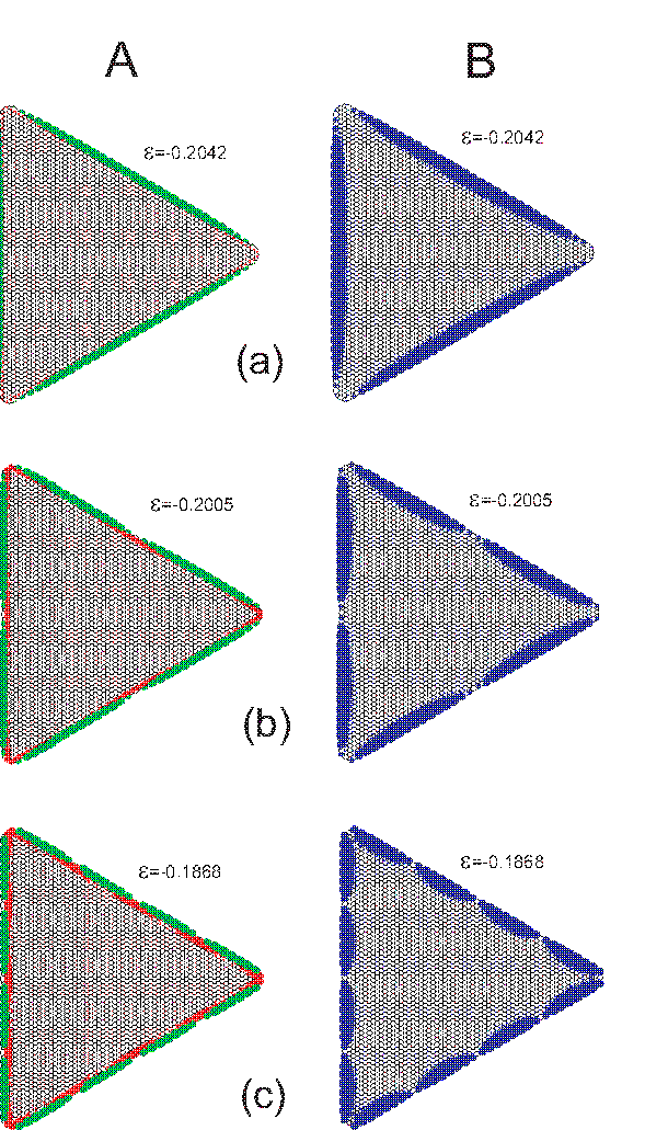
Figure 6: (Color online) TB electron densities (modulus) of reczag edge states participating (counting from the bottom) in the first (a), second (b), and fourth (c) braid bands of region D1 [see Fig. 5(a)], at $\Phi=15.9\Phi_{0}$. The A (red) and B (blue) sublattices are plotted separately. Green color denotes the density on the outer carbon dimers resulting from the edge reconstruction and connected by the hopping matrix element $t_{4}$ in Fig. 1. (Note that the color codings between Fig. 1 and the current Fig. 6 are unrelated). The presence of azimuthal (along the sides of the triangle) nodes in the electronic densities is clearly visible. The number of nodes changes by unity from one braid band to the next, increasing with increasing energy. This behavior (including the fact that all three states within each braid band maintain the same number of nodes) is quite analogous to that of the edge states of a trigonal graphene nanoring at low magnetic fields (see Fig. 7 below). Energies in units of $t=2.7$ eV.

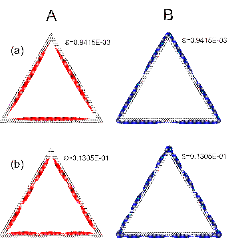
Figure 7: (Color online) TB electron densities (modulus) of edge states of the zigzag ring participating (counting from the bottom) in (a) the first and (b) the third braid bands in Fig. 5(b)], at $\Phi/\Phi_{0}\sim 6$. The A (red) and B (blue) sublattices are plotted separately. The azimuthal nodes in the electronic densities are clearly visible. The number of nodes changes by one from one braid band to the next, increasing with increasing energy. Energies in units of $t=2.7$ eV. The ring has a total of 906 carbon atoms.

An enlarged section of the electronic spectrum in Fig. 3(c) (case of type-I corner) is displayed in Fig. 4(a), while the corresponding section for a trigonal reczag QD with type-II corners is displayed in Fig. 4(b). From a comparison of the two cases in Fig. 4, we conclude that the main features in the region D maintain: they show rather small variations between the type-I and type-II corners. The larger variation is exhibited by the E1 regime (not shown in Fig. 4). Indeed the E1 line for the type-II corners has moved to a positive energy $\varepsilon_{c}\approx 0.120t$. The enlarged spectra in Fig. 4 suggest a further division of the D regime into features denoted as D1, D2, and E2. (The grouping of the E2 feature with the E1 feature will become apparent below; see Sec. III.2.4).

Because of the similarity between the electronic spectra of the two types of corners, it will be sufficient below to restrict our further analysis of spectral features to the case of type-I corners [see Fig. 4(a) and Fig. 3(c)].

III.2.1 Region D1: Ideal-ring, low-$B$-type edge states and Aharonov-Bohm oscillations

The main feature of the D1 region are the many energy bands consisting of three-curve braid patterns, an enlargement of which is displayed in Fig. 5(a). These braid bands are quite similar to the ones displayed by the low-$B$ electronic spectra of a narrow trigonal graphene nanoring with zigzag edges [see Fig. 5(b)], which were investigatedroma12 recently in the context of the AB effect. Based on this similarity and the findings of Ref. roma12, , we infer that these braid bands are associated with the formation of a second type of edge states, in addition to the Halperin-type ones. This second type edge states are localized (in the radial direction) within the physical defective reczag edge and exhibit behavior associated with a quantum wire. In particular, in the case of a trigonal reczag-GQD, the three wire segments along the sides of the triangle are coupled pairwise (via electron tunneling at the corners) and form a trigonal quantum nanoring. Henceforth, we will adopt the term reczag edge states to designate these states, which are associated with the physical defective edge.

To gain further insight into the similarity of the reczag edge states to the graphene-ring states, we display in Fig. 6 the probability densities at $\Phi/\Phi_{0}=15.9$ ($\phi/\Phi_{0}=0.0037$) for several of the reczag states [with energies belonging to successive braid bands starting with the lowest-in-energy one; see Fig. 5(a)]; $\phi$ denotes the magnetic flux through a single hexagon of the honeycomb graphene lattice. Probability densities at $\Phi/\Phi_{0}\sim 6$ ($\phi/\Phi_{0}=0.003$) for two characteristic states of the narrow trigonal graphene nanoring with zigzag edges (considered in Ref. roma12, ) are displayed in Fig. 7. It is apparent that the electronic densities in Fig. 6 (reczag flake) are restricted near the physical boundary of the flake, and thus they correspond to formation of edge states. In addition, the presence of azimuthal (along the sides of the triangle) nodes in these electronic densities is clearly visible, and the number of nodes changes by unity from one braid band to the next, increasing with increasing energy. This behavior (including the fact that all three states within each braid band maintain the same number of azimuthal nodes) is quite analogous to that of the edge states of a trigonal graphene nanoring at low magnetic fields (see Fig. 7).

The similarities between the reczag edge states and the low-$B$ states of graphene nanorings indicates that the reczag edge behaves like a quantum wire. Naturally, this quantum-wire behavior places the reczag edge states in a separate category, different from that of the Halperin-type edge states. In Sec. III.2.2 below, we will further elaborate on the quantum-wire aspects of the reczag edge states using a simple one-dimensional superlattice model.

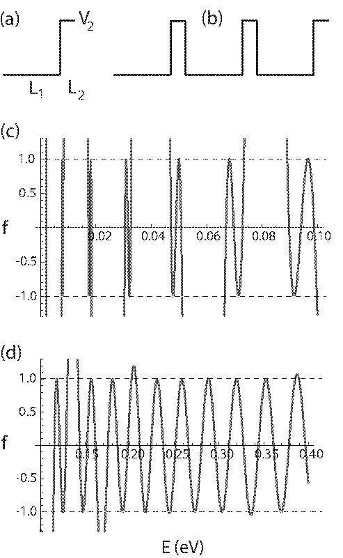
Figure 8: (Color online) (a) Schematic diagram of the unit subcell associated with a single side of the trigonal graphene flake with reczag edge terminations. $V_{2}$ denotes the height of the potential barrier which mimicks the scatterer at the corners of the trigonal reczag flake. (b) Schematic diagram of the unit cell associated with the magnetic-field virtual lattice; it involves all three sides of the equilateral triangle, and thus it consists of three unit subcells in a series. (c)-(d) The function $f(E)=\operatorname{Tr}[{\bf T}(E)]/2$ [see the r.h.s. of Eq. (7)], which is associated with the unit cell [shown in (b)] of the magnetic-field virtual superlattice, as a function of the energy variable $E$. In calculating $f(E)$, the parameters for the unit subcell [shown in (a)] were taken as: $L_{1}=12.5$ nm, $L_{2}=1.5$ nm, $V_{1}=0$, and $V_{2}=0.1$ eV. The relevant values of $f(E)$ lie within $\pm 1$ (i.e., within the dotted lines). (c) $f(E)$ in the range $0\leq E\leq V_{2}$. (d) $f(E)$ in the range $V_{2}\leq E\leq 4V_{2}$. Energy in units of eV.

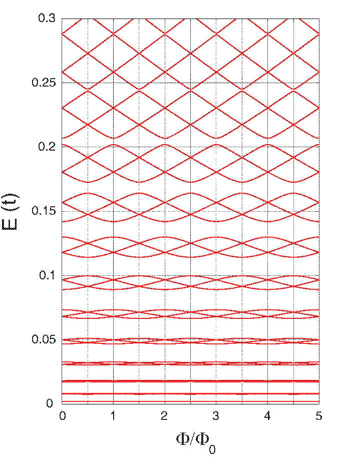
Figure 9: (Color online) Single-particle spectrum (as a function of the total flux $\Phi$) from the semianalytic superlattice model considered in Sec. III.2.2. The parameters for the unit subcell mimicking each reczag side of the trigonal graphene flake are: $L_{1}=12.5$ nm, $L_{2}=1.5$ nm, $V_{1}=0$, and $V_{2}=0.1$ eV. Note that the total length $L_{1}+L_{2}=14$ nm is similar to the length of the trigonal flake in Fig. 3. The height of the potential barrier defining the scatterers at the corners $(V_{2})$ is roughly one fifth of the width ($0.2t$) of the D region [see Fig. 3(c)]. Energies in units of eV. The magnetic flux is given in units of $\Phi_{0}=hc/e$.

III.2.2 A simple semianalytic model for the reczag edge states

In this section we show that the main qualitative features of the braid bands in the D1 region can be reproduced using a simple nonrelativistic 1D superlattice approach. Indeed, in this approach, each side of the trigonal reczag flake is modeled as a unit subcell consisting of a two-region piece-wise potential [see Fig. 8(a)]. In particular, the first and wider region was chosen to have a length of $L_{1}=12.5$ nm and a zero potential height, $V_{1}=0$. The second region models the scatterer’s behavior of the triangle’s corner and was taken to be a narrow potential barrier; we chose $L_{2}=1.5$ nm and $V_{2}=0.1$ eV. Note that the total length $L=L_{1}+L_{2}=14$ nm is similar to the length of the side of the equilateral triangle in Fig. 3, while the height of the potential barrier is roughly one fifth of the width ($0.2t$) of the D region (see Fig. 3). Naturally, due to the simplicity of the model, we did not attempt to achieve a full quantitative agreement with the TB spectra.

Following Ref. gilmbook, , one constructs first the transfer matrices ${\bf M}_{1}$ and ${\bf M}_{2}$ (see the Appendix) for the regions 1 and 2 of the unit subcell portrayed in Fig. 8(a). Then the transfer matrix (${\bf T_{s}}$) for the unit subcell is simply the product of the two matrices ${\bf M}_{1}$ and ${\bf M}_{2}$, i.e.,

$${\bf T_{s}}={\bf M}_{1}{\bf M}_{2}.$$ (5)

A magnetic field perpendicular to the plane generates a flux $\Phi$ over the entire area of the flake. Thus all three sides of the triangle must be considered in the study of magnetic-field effects. To this end, and following Ref. imry83, , we consider the equivalent problem of a magnetic-field virtual superlattice. In our case, however, the unit cell of the virtual lattice is more complex; it consists of three unit subcells in a series [see Fig. 8(b)] in order to account for the three scatterers at the corners. Then the transfer matrix for the unit cell is given by

$${\bf T}={\bf T_{s}}^{3}.$$ (6)

To form the magnetic-field superlattice, the unit cell must be repeated ad-infinitum. This is equivalent to imposing periodic boundary conditions on a succession of finite lattice blocks with ${\cal N}$ unit cells and taking the limit ${\cal N}\rightarrow\infty$. Accordingly,gilmbook the dispersion relation determining the energy bands of the virtual superlattice is given by

$$\cos(2\pi\Phi/\Phi_{0})=\operatorname{Tr}[{\bf T}(E)]/2,$$ (7)

where we used the fact that the equivalent Bloch wave vector for the magnetic-field superlattice is ${\cal K}=2\pi\Phi/(3L\Phi_{0})$, $3L$ being the width of the unit cell (see Ref. imry83, ).

The energy bands resulting from the dispersion relation in Eq. (7), with the specific parameter values mentioned in the beginning of this section, are displayed in Fig. 9. A comparison with the braid bands in Figs. 4(a) and 5(a) (D1 region of the TB spectra) shows that the simple 1D model reproduces the essential trends of the TB braid bands. Specifically, the common trends are as follows: (I) The alternation 2-1-1-2 (1-2-2-1) in the state degeneracy between two successive braid bands at $\Phi/\Phi_{0}=n$ ($\Phi/\Phi_{0}=n+1/2$), $n=0,1,2,\ldots$ [see the horizontal arrows in Fig. 5(a) and Fig. 9]. (II) The width of the braid bands increases with increasing energy. (III) In contrast, the energy gaps separating the braid bands decrease with increasing energy. (IV) At high enough energies, the braid bands tend to merge into a single pattern having “chicken-wire” topology, familiar from the well-known ideal-metal-ring energy spectrum;cheu88 this last feature is present in the TB spectra of Fig. 4 in the region $0\leq\Phi/\Phi_{0}<8.0$.

We note that in the context of the simple 1D model of this section, these trends can be further understood from an inspection of the behavior of the $f(E)$ function plotted in Fig. 8(c) and Fig. 8(d). Indeed, for a given $\Phi$, the single-particle energies plotted in Fig. 9 correspond to the crossing points of the $f(E)$ curve with a horizontal straight line having an ordinate $f=\cos(2\pi\Phi/\Phi_{0})<1$. In particular, the trend No. IV above is associated with the asymptotic behavior of the $f(E)$ function; this asymptotic behavior at high energies (above the barrier height $V_{2}$) corresponds to the fact that the tunneling particle behaves like a free fermion and it does not feel strongly the effect of the scatterers.

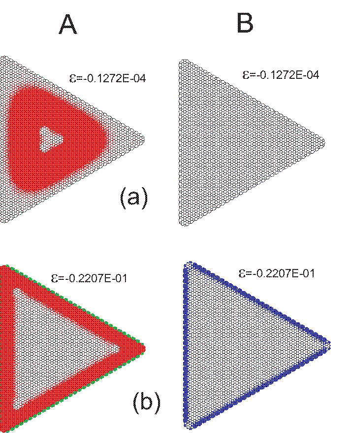
Figure 10: (Color online) TB electron densities (modulus) of two characteristic states for the D2 regime of the reczag flake at $\Phi/\Phi_{0}=15.9$. (a) a state with near-zero energy $\varepsilon=-0.1272\times 10^{-4}t$ exhibiting bulk zero-Landau-level behavior. (b) a state with lower energy $\varepsilon=-0.2207\times 10^{-1}t$ exhibiting Halperin-edge behavior. Compared to Fig. 6, the absence of azimuthal nodes in the electronic densities here is noticeable. Energies in units of $t=2.7$ eV. The total number of carbon atoms is 4731. The A (red) and B (blue) sublattices are plotted separately. Green color denotes the density on the outer carbon dimers resulting from the edge reconstruction and connected by the hopping matrix element $t_{4}$ in Fig. 1.

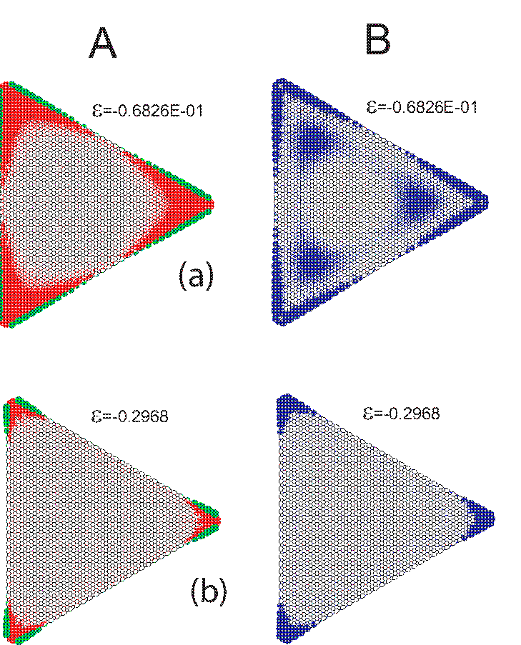
Figure 11: (Color online) TB electron densities (modulus) of two characteristic states for the E1 and E2 regimes of the reczag flake at $\Phi/\Phi_{0}=15.9$. Note the concentration of the electron densities at the corners of the triangle. (a) a state in the E2 regime with energy $\varepsilon=-0.6826\times 10^{-1}t$. (b) a state in the E1 regime with energy $\varepsilon=-0.297t$. Energies in units of $t=2.7$ eV. The A (red) and B (blue) sublattices are plotted separately. Green color denotes the density on the outer carbon dimers resulting from the edge reconstruction and connected by the hopping matrix element $t_{4}$ in Fig. 1.

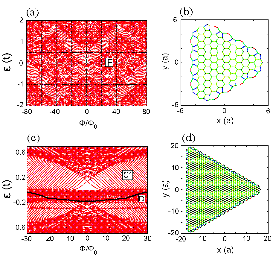
Figure 12: (Color online) (a) TB single-particle spectrum for a very small (with type-I corners) reczag trigonal graphene dot, as a function of the magnetic field (the magnetic flux $\Phi$ over the whole dot). (b) Shape of the equilateral trigonal graphene dot which corresponds to (a); it has 10 hexagons in the outer unreconstructed row along each side (the total number of carbon atoms is 195). (c) TB single-particle spectrum for a larger (with type-I corners) reczag trigonal graphene dot, as a function of the magnetic field (the magnetic flux $\Phi$ over the whole dot). (d) Shape of the trigonal graphene dot which corresponds to (c); it has 38 hexagons in the outer unreconstructed row along each side (the total number of carbon atoms is 1819). The thick black line in (c) denotes the Fermi level in the canonical ensemble corresponding to $N=60$ holes (spin included). Energy in units of the tight-binding hopping-parameter $t=2.7$ eV. Lengths in units of the honeycomb graphene lattice constant $a=0.246$ nm. The magnetic flux is given in units of $\Phi_{0}=hc/e$.

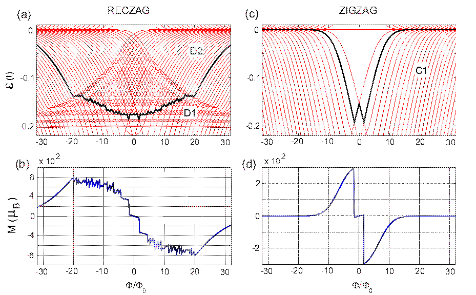
Figure 13: (Color online) (a) Reczag flake: An enlarged part of the TB single-particle spectrum shown in Fig. 12(c), as a function of the magnetic field (the magnetic flux $\Phi$ over the whole dot). The shape of the corresponding reczag flake is displayed in Fig. 12(d). (b) Reczag flake: Landau magnetization (at zero temperature) for $N=60$ holes (spin included) exhibiting Aharonov-Bohm oscillations superimposed on larger ones generated by the rapid variation of the background Halperin-type edge states which cross the braid bands. The thick black line in (a) denotes the corresponding Fermi level in the canonical ensemble. (c) Zigzag flake: A similar part of the TB single-particle spectrum for the corresponding zigzag trigonal flake (with 38 hexagons in the outer row along each side), as a function of the magnetic flux $\Phi$. (d) Zigzag flake: Landau magnetization for $N^{*}=4$ effective holes (spin included); the absence of Aharonov-Bohm oscillations is apparent. The thick black line in (c) denotes the corresponding Fermi level in the canonical ensemble. For a meaningful comparison, this Fermi level was chosen to fall within the $\varepsilon_{b}=-0.205t<\varepsilon<0$ energy band. Note that for the reczag flake this energy band contains the special D region; for the zigzag flake this energy band is reduced to being part of region C1. The total number of holes is $N=N_{0}+N^{*}$, where $N_{0}$ is the number of strictly zero-energy states present in the zigzag trigonal flake (also, see text). Energy in units of the tight-binding hopping-parameter $t=2.7$ eV. The magnetic flux is given in units of $\Phi_{0}=hc/e$.

III.2.3 Region D2: Dense spectrum of Halperin-type edge states

We focus now on the region marked as D2 in Fig. 4(a). The single-particle spectra in this region consist of energy curves similar to those of the Halperin-type edge states in region C1 (which connect the $n=1$ and $n=0$ graphene Landau levels). A main difference, however, between these two regions is that the spectrum in D2 is more dense compared to that in region C1. For example, at $\Phi/\Phi_{0}=15.9$, we found that within the range $|\varepsilon|\leq 0.4414t$, there are 20 states in the D2 region, but only 10 states in the C1 region above the zero-energy line. We note that the density of states in the C1-region of a reczag flake is similar to that in the C1-region of a zigzag flake with comparable size. As a result, because all the states in region D2 converge to the zero-energy Landau level, the degeneracy (density of states per unit magnetic flux) of this Landau level is higher in the case of a trigonal reczag flake compared to that of a pure zigzag flake. This behavior raises naturally the question of whether the conductance properties of the anomalousgeim09 ; aban06 ; brey06.2 relativistic IQHE will be impacted. We will, however, defer elaborating on this question until the section on the continuous Dirac-Weyl description (Sec. IV).

To further investigate the properties of region D2, we display (for $\Phi/\Phi_{0}=15.9$) in Fig. 10 electron densities for a couple of characteristic states in this region. Compared to Fig. 6, the absence of azimuthal nodes in their electronic densities is noticeable. Specifically,, in Fig. 10(a) we consider a state with near-zero energy ($\varepsilon=-0.1272\times 10^{-4}t$). This state exhibits a zero-Landau-level behavior familiar from a graphene sheet,geim09 and accordingly, one sublattice component (here the B-sublattice) vanishes everywhere. This contrasts with the special case of the zero-Landau-level states in a zigzag flake, which are of a mixed bulk-edge character, with the bulk and edge components residing on different sublattices. yann10 ; roma11 In Fig. 10(b), we consider a state with lower energy $\varepsilon=-0.2207\times 10^{-1}t$, which is representative of the pristine Halperin-type double-edge states between the $n=0$ and $n=1$ Landau levels discussed in Refs. yann10, ; roma11, for GQDs with zigzag edge terminations.

The enhanced density of TB states in the D2 region maintains also in the spectra derived from the continuous Dirac-Weyl equation in the case of a circular disk with reczag edges (see Sec. IV below).

III.2.4 Regions E1 and E2: States localized at the corners

The states belonging to the E1 and E2 regimes are grouped together. Indeed, as revealed from the electron densities displayed in Fig. 11, they are localized (to one degree or the other) at the corners of the triangle. As seen from Fig. 4(a), the E2 feature consists of three states whose energy curves form a single braid, similar to the braids in region D1. One of the states in this triad (with energy $\varepsilon=-0.6826\times 10^{-1}t$ at $\Phi/\Phi_{0}=15.9$) is plotted in Fig. 11(a). Because of the localization at the corners, the quantum-wire model of Sec. III.2.2 is not appropriate for the E2 regime. However, as discussed in Sec. IV A of Ref. yann03, (see in particular Figs. 6 and 7 therein), a simple Hückel model involving three localized Gaussian wave functions at the corners of an equilateral triangle is able to reproduce qualitatively the braiding behavior of the energy curves as a function of the magnetic field.

The states in the E1 regime behave in a different way; in fact, their energies as a function of $B$ do not form a braid, but an approximate straight line located at $\varepsilon_{c}\approx-0.297t$. In the C2 region (between the $n=-2$ and $n=-1$ Landau levels), there are three such states with very close energies [at $\Phi/\Phi_{0}=15.9$, these energies are $-0.2957t$, $-0.2968t$, and $-0.2976t$; the state corresponding to the second energy here is plotted in Fig. 11(b)]. In the C1 region (between the $n=-1$ and $n=0$ Landau levels), only two of these states exist. At present, we are unaware of any simple model describing such a behavior.

Because the corners were shown earlier to act as scatterers (see Sec. III.2.2), the appearance of states that are localized at (or attracted towards) the corners may seem counterintuitive at a first glance. This behavior, however, originate from the relativistic nature of the graphene massless Dirac quasiparticles for which the scatterers may also act as centers of attraction due to Klein tunneling.klei29 ; kats06 In this context, we mention Ref. kim10, , where similar localized wave functions under the repulsive potential barrier defining a circular graphene antidot were reported.

III.3 Smaller trigonal shapes and Aharonov-Bohm oscillations

Of interest is the question of the size-dependence of the spectra of the reczag trigonal flakes. The size of the flake investigated in previous sections [with sixty hexagons along each side, see Fig. 3(d)] is sufficiently large for the main features of the spectra to have been fully developed. We thus briefly investigate here smaller sizes. Indeed, Fig. 12(a) displays the spectrum of a very small trigonal reczag flake with 10 hexagons along each side [see the corresponding shape in Fig. 12(b)], while Fig. 12(c) displays the spectrum of an intermediate-size flake with 38 hexagons along each side [see the associated shape in Fig. 12(d)].

The spectrum for the very small flake [Fig. 12(a)] exhibits rather large differences from that of the large flake [Fig. 3(c)]. This is mainly due to the full development (within the plotted $\Phi$ range) of the Hofstadter-butterflyhofs76 ; zhan08 fractal patterns (designated as region F), which appear for very strong magnetic fields such that $l_{B}\lesssim a$, i.e., when the magnetic length is similar to or smaller than the honeycomb graphene-lattice constant. Furthermore the Landau levels (region B) and region D (which is unique to the reczag edges and has been our main focus in this paper) are hardly recognizable; they are strongly quenched compared to the case of the large flake in Fig. 3(c).

For the intermediate-size case shown in Fig. 12(c), both the Landau-level regime and the two regimes D1 (three-member braid bands) and D2 (Halperin-type edge states with enhanced density) are well developed; see enlarged part in Fig. 13(a). We note again the constancy and size-independence of the lower bound $\varepsilon_{b}$ of the D region.

We take advantage of the full development of the spectrum in the intermediate size, and we calculate explicitly for this size the Landau magnetization [displayed in Fig. 13(b)] for a positively charged flake with $N=60$ holes (spin included). Following Ref. roma12, , we carry out this calculation in the canonical ensemble and zero temperature, and the thick black line in Fig. 13(a) denotes the corresponding Fermi level. As a function of the total magnetic flux $\Phi$, the magnetization exhibits clear (albeit with variable shapes) oscillatory Aharonov-Bohm patterns associated with the braid bands. At the same time, these AB patterns are superimposed on larger oscillations generated by the rapid variation (with $\Phi$) of background Halperin-type edge states crossing the braid bands. These background Halperin edge states are also responsible for the skipping of the Fermi level between different braid bands and between different states in the same braid band, which results in the jumps and in the variation of the shape of the AB patterns (which is to be contrasted with the regular AB oscillations in graphene nanorings with zigzag edges roma12 ).

We display also in Fig. 13(c) and Fig. 13(d) the energy spectrum and Landau magnetization, respectively, for the corresponding zigzag trigonal flake (with 38 hexagons in the outer row along each side). The absence of Aharonov-Bohm oscillations in Fig. 13(d) is apparent. For a meaningful comparison, the Fermi level in the canonical ensemble [see thick black line in (c)] was chosen to fall within the $\varepsilon_{b}=-0.205t<\varepsilon<0$ energy band. We note that for the reczag flake this energy band contains the special D region; for the zigzag flake this energy band is reduced to being part of region C1. For the zigzag flake the Fermi level is determined by the number $N^{*}$ of effective holes ($N^{*}=4$ here, spin included). Indeed the total number of holes is $N=N_{0}+N^{*}$, with $N_{0}$ being the number of strictly zero-energy states present in the zigzag trigonal flake ($N_{0}$ equalspala07 ; pota10 the number of hexagons along one side minus one). Naturally, the strictly zero-energy states do not contribute to the Landau magnetization. We further note that as a result of the reconstruction process (reczag flake), however, the strictly zero-energy states acquire finite energies. In a continuum model (see Sec. IV below), this mapping is codified by the boundary condition specified by Eq. (8), which involves the reczag parameter ${\cal F}$ [Eq. (9)]; for ${\cal F}=0$, the zigzag-edge case is recovered.

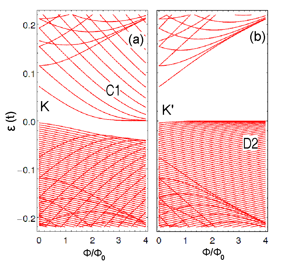
Figure 14: (Color online) Single-particle spectra as a function of the magnetic flux $\Phi$, according to the continuous Dirac-Weyl description for a circular GQD with a reczag edge termination. (a) The $K$ valley. (b) The $K^{\prime}$ valley. The radius of the dot is $R=8$ nm. Energies in units of $t=2.7$ eV.

IV Continuous Dirac-Weyl description for circular reczag GQDs

In order to describe the properties of graphene and graphene nanosystems near the neutral Dirac point, the continuous Dirac-Weyl equation has been widely and successfully used as an alternative to the TB calculations. In particular for graphene nanoribbons with zigzag and armchair edge terminations there is an overall agreement between the TB results and those of the DW approach. Although the shape of a GQD in the continuous description is most often taken as circular and not polygonal, this overall agreement (albeit with certain caveats) between circular and TB calculations was also found to extend to the case of graphene nanoflakes and nanodots (see, e.g., Ref. roma11, ). It is thus of interest to investigate whether such overall agreement applies also for the unique features of a reczag flake discussed in earlier sections.

In the continuum approach, a graphene Dirac electron (or hole) is represented by a four-component spinor $(\Psi_{A},\Psi_{B},\Psi^{\prime}_{A},\Psi^{\prime}_{B})^{T}$, with the indices A and B denoting the two sublattices, and the unprimed and primed symbols denoting the $K$ and $K^{\prime}$ valleys. In the case of zigzag or armchair edge terminations, the four components of the spinor obey well-known characteristic boundary conditions.mont10 ; geim09 ; brey06 For the case of the reczag edge, corresponding boundary conditions were proposed recently in Ref. osta11, . For the $K$ valley these conditions relate the components on the A and B sublattices as follows:

$$\Psi_{A}=i{\cal F}\Psi_{B},$$ (8)

where the parameter ${\cal F}$ is defined as

$${\cal F}=\frac{t_{1}^{2}t_{4}(t_{2}t_{4}-t_{3}^{2})}{2t(t_{3}^{4}+t_{2}t_{3}^{2}t_{4}+t_{2}^{2}t_{4}^{2})}.$$ (9)

The value for ${\cal F}=0.07$ for the reczag edge; see Table 1 for the values of the hopping matrix elements $t_{k}$, $k=1,2,3,4$. For the $K^{\prime}$ valley, the boundary condition is obtained via the substitution ${\cal F}\rightarrow-1/{\cal F}$. Note that the reczag edge does not mix the two valleys,osta11 as is the case with the zigzag boundary condition.

For a finite circular graphene sample of radius $R$, we seek solutions of Eq. (4) for $\varepsilon\neq 0$ that are regular at the origin ($x=0$). For a nanodot with a reczag edge one finds that the single-particle spectrum is given by the solutions of the following dispersion relation:

$$\chi_{B}(\varepsilon,m,x)+{\cal F}\chi_{A}(\varepsilon,m,x)=0,$$ (10)

where ${\cal F}=0.07$ for the $K$ valley and ${\cal F}=-1/0.07$ for the $K^{\prime}$ valley, $x=R/l_{B}$, $m$ is an angular momentum, and (see Ref. yann10, )

$$\chi_{A}(\varepsilon,m,x)\propto\left\{\begin{array}[]{cc}x^{m}e^{-x^{2}/4}M(m+1-\frac{\varepsilon^{2}}{2},m+1,\frac{x^{2}}{2});&\;\text{if}\;\;m\geq 0\\ x^{-m}e^{-x^{2}/4}M(1-\frac{\varepsilon^{2}}{2},-m+1,\frac{x^{2}}{2});&\;\text{if}\;\;m\leq-1\end{array}\right.$$ (11)

and

$$\chi_{B}(\varepsilon,m,x)\propto\left\{\begin{array}[]{cc}\frac{\varepsilon}{2}\frac{x^{m+1}}{m+1}e^{-x^{2}/4}M(m+1-\frac{\varepsilon^{2}}{2},m+2,\frac{x^{2}}{2});&\;\text{if}\;\;m\geq 0\\ \frac{2m}{\varepsilon}x^{-m-1}e^{-x^{2}/4}M(-\frac{\varepsilon^{2}}{2},-m,\frac{x^{2}}{2});&\;\text{if}\;\;m\leq-1\end{array}\right.,$$ (12)

where $M(a,b,z)$ is Kummer’s confluent hypergeometric function. abrabook

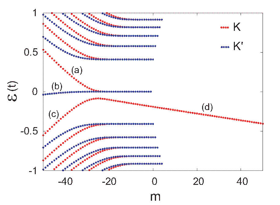
Figure 15: (Color online) Single-particle energies as a function of the angular momentum $m$, according to the continuous Dirac-Weyl description for a circular GQD with a reczag edge termination. The total flux is fixed at $\Phi=15\Phi_{0}$. Both the $K$ and $K^{\prime}$ valleys are considered. Note the four dispersive branches of edge states [(a), (b), (c), and (d)] associated with the zeroth Landau level. We note that only two dispersive branches of edge states [(a) and (c)], associated with the zeroth Landau level, appear in a circular GQD with a zigzag edge termination. The radius of the dot is $R=8$ nm. Energies in units of $t=2.7$ eV.

The solutions of the dispersion relation in Eq. (10) are plotted in Fig. 14(a) for the $K$ valley and in Fig. 14(b) for the $K^{\prime}$ valley. One observes that the general features discussed in Sec. III.1 (namely, the Landau levels, and the Halperin-type edge states) are also present in the continuum-DW reczag spectra. However, concerning the unique features found via TB calculations [Sec. III.2] and associated with a trigonal reczag flake, only the feature of the Halperin-type edge states with an enhanced density spectrum (D2 region) maintains also in the continuum spectra [see Fig. 14(b)]. The rest of the special reczag features are missing in Fig. 14: in particular we note the nonexistence of a lower-energy bound $\varepsilon_{b}$ for the D region and the absence of the three-member braid bands (region D1), the latter being a reflection of the ability of the defective reczag edge to behave as a 1D quantum nanoring. Furthermore, we note that the E1 and E2 states, which are localized at the corners, are also missing in the continuum model.

Due to these major discrepancies between the TB and continuum descriptions, we are led to conclude that the linearized DW equation fails to capture essential nonlinear physics resulting from the introduction of a nontrivial defect in the honeycomb graphene lattice. Indeed the Dirac-Weyl equation is obtained for the low-energy states of electrons in the honeycomb lattice, and it is not valid at the reczag edges and the corners, where the topological structures are very different from the honeycomb lattice.

As mentioned earlier in Sec. III.2.3, the presence of Halperin-type edge states with an enhanced density spectrum (D2 region) raises naturally the question whether this feature may impact the conductance behavior of the anomalousgeim09 ; aban06 ; brey06.2 relativistic IQHE. To be able to answer this question within the continuous DW description, one needs to count the dispersive branches of edge states present in the spectrum of the circular reczag dot when the single-particle energies are plotted versus the angular momentum $m$ and at a fixed value of the magnetic flux (the magnetic field). For a circular reczag GQD with radius $R=8$ nm (as was the case in Fig. 14 where the magnetic flux was varied), this latter spectrum is displayed in Fig. 15 (for a fixed magnetic flux $\Phi=15\Phi_{0}$). Both the $K$ and $K^{\prime}$ valleys are considered. We note that there are four dispersive branches [labeled as (a), (b), (c), and (d)] associated with the zeroth Landau level. Furthermore, it was found that all four channels represent edge states; see also Ref. osta11, where the case of the linear reczag edge of a semi-infinite graphene plane was considered. In contrast, only two dispersive branches [corresponding to (a) and (c)], associated with the zeroth Landau level, appear in a circular GQD with a zigzag edge termination.aban06 ; brey06.2 The appearance of these four branches in the spectrum of the circular reczag GQD, however, does not influence the IQHE conductance, because two of them, i.e., the (c) and (d) are counter propagating, and thus their contributions are expected to cancel each other.

We stress, however, that the above conclusion is based on the continuous DW spectrum. As noted above, the DW spectrum differs drastically from the TB one, and thus a definitive answer to the question concerning the IQHE-conductance behavior associated with a trigonal reczag flake requires a full study of the current/transmission using the tight-binding method.roma13

V Summary and discussion

The electronic spectra of graphene nanoflakes with reczag edges, where a succession of pentagons and heptagons, that is 5-7 topological defects, replaces the hexagons at the familiar zigzag edge, were investigated via systematic tight-binding calculations. Three different sizes of trigonal graphene flakes were considered in Sec. III, with the two smaller sizes being discussed in Sec. III.3. (A detailed recapitulation of the results was given in Sec. I.3 of the Introduction.) Emphasis was placed on topological aspects and connections underlying the patterns dominating these spectra. A central result is that the spectra of trigonal reczag flakes exhibit both general features (Sec. III.1), which are shared with GQDs having other edge terminations (i.e., zigzag or armchair), as well as special ones (Sec. III.2), which are unique to the reczag edge termination. These unique features include breaking of the particle-hole symmetry, and they are associated with a nonlinear dispersion of the energy as a function of momentum, which may be interpreted as nonrelativistic behavior.

The general topological features (Sec. III.1) shared with the zigzag flakes include the appearance of energy gaps at zero and low magnetic fields due to finite size, the formation of relativistic Landau levels at high magnetic fields, and the presence between the Landau levels of Halperin-type edge states associated with the integer quantum Hall effect. Topological regimes, unique to the reczag nanoflakes (Sec. III.2), appear within a stripe of negative energies $\varepsilon_{b}=-0.205t<\varepsilon<0$, and along a separate feature forming a constant-energy line outside this stripe.

Prominent among the patterns within the $\varepsilon_{b}=-0.205t<\varepsilon<0$ energy stripe is the formation of three-member braid bands, resembling those in the spectra of narrow graphene nanorings (Sec. III.2.1). The reczag edges along the three sides of the triangle act as a one-dimenional quantum wire (with the corners behaving as scatterers) enclosing the magnetic flux through the entire area of the graphene flake (Sec. III.2.2). This leads to the development of Aharonov-Bohm-type oscillations in the magnetization (Sec. III.3). Another prominent feature within the $\varepsilon_{b}=-0.205t<\varepsilon<0$ energy stripe is a subregion of Halperin-type edge states of enhanced density immediately below the zero-Landau level (Sec. III.2.3). Furthermore, there are features resulting from localization of the Dirac quasiparticles at the corners of the polygonal flake (Sec. III.2.4).

A main finding concerns the limited applicability of the continuous Dirac-Weyl equation in conjuntion with the boundary condition proposed in Ref. osta11, . Indeed, this combination does not reproduce the special reczag features. Due to this discrepancy between the tight-binding and continuum descriptions, one is led to the conclusion that the linearized Dirac-Weyl equation fails to capture essential nonlinear physics resulting from the introduction of a multiple topological defect in the honeycomb graphene lattice.

We comment here that simpler topological defects (e.g., a singlebern08 pentagon, heptagon, or pentagon-heptagon pair embedded in the honeycomb lattice) are often describedmesa09 ; vozm10 (at zero magnetic field) in the continuum DW approach via a gauge field (an additional vector potential) resembling the one generated by an Aharonov-Bohm magnetic-flux solenoid. The generalization of this gauge-field modification of the DW equation to multiple topological defects may provide a better overall agreement with the TB results.

*

Appendix A Expressions for the transfer matrices

For the first region of the unit subcell in Fig. 8(a), the transfer matrix is gilmbook

$${\bf M}_{1}=\left(\begin{array}[]{cc}\cos(k_{1}L_{1})&-\sin(k_{1}L_{1})/k_{1}\\ k_{1}\sin(k_{1}L_{1})&\cos(k_{1}L_{1})\end{array}\right),$$ (13)

with $k_{1}=\sqrt{2mE/\hbar^{2}}$; $m$ is the nonrelativistic electron mass and $E$ the energy variable.

For the second region of the unit subcell, the transfer matrix isgilmbook

$${\bf M}_{2}=\left(\begin{array}[]{cc}\cosh(\kappa_{2}L_{2})&-\sinh(\kappa_{2}L_{2})/\kappa_{2}\\ -\kappa_{2}\sinh(\kappa_{2}L_{2})&\cosh(\kappa_{2}L_{2})\end{array}\right),$$ (14)

with $\kappa_{2}=\sqrt{2m(V_{2}-E)/\hbar^{2}}$, if $E<V_{2}$, and

$${\bf M}_{2}=\left(\begin{array}[]{cc}\cos(k_{2}L_{2})&-\sin(k_{2}L_{2})/k_{2}\\ k_{2}\sin(k_{2}L_{2})&\cos(k_{2}L_{2})\end{array}\right),$$ (15)

with $k_{2}=\sqrt{2m(E-V_{2})/\hbar^{2}}$, if $E\geq V_{2}$.

Using the matrices ${\bf M}_{1}$ and ${\bf M}_{2}$ defined above, and with the help of the algebraic language MATHEMATICA,math we found that the trace of the transfer matrix ${\bf T}$ [see Eqs. (5) $-$ (7)], which is associated with the unit cell of the virtual magnetic superlattice, is given by

$$\operatorname{Tr}[{\bf T}(E)] = \left\{2k_{1}^{3}\kappa_{2}^{3}\cos(3k_{1}L_{1})\cosh^{3}(\kappa_{2}L_{2})+3k_{1}^{2}\kappa_{2}^{2}(-k_{1}^{2}+\kappa_{2}^{2})\cosh^{2}(\kappa_{2}L_{2})\sin(3k_{1}L_{1})\sinh(\kappa_{2}L_{2})+\right.$$ (16)

$$3k_{1}\kappa_{2}\cos(k_{1}L_{1})\biglb(k_{1}^{4}+\kappa_{2}^{4}-(k_{1}^{2}-\kappa_{2}^{2})^{2}\cos(2k_{1}L_{1})\bigrb)\cosh(\kappa_{2}L_{2})\sinh^{2}(\kappa_{2}L_{2})+$$

$$\left.(k_{1}^{2}-\kappa_{2}^{2})\biglb(-3(k_{1}^{2}+\kappa_{2}^{2})^{2}\sin(k_{1}L_{1})+(k_{1}^{2}-\kappa_{2}^{2})^{2}\sin(3k_{1}L_{1})\bigrb)\sinh^{3}(\kappa_{2}L_{2})/4\right\}/(k_{1}^{3}\kappa_{2}^{3}),$$

when $E<V_{2}$, and

$$\operatorname{Tr}[{\bf T}(E)] = -\left\{-2k_{1}^{3}k_{2}^{3}\cos^{3}(k_{1}L_{1})\cos(3k_{2}L_{2})+\right.$$ (17)

$$\left.3k_{1}k_{2}\cos(k_{1}L_{1})\cos(k_{2}L_{2})\biglb(-k_{1}^{4}-k_{2}^{4}+(k_{1}^{2}+k_{2}^{2})^{2}\cos(2k_{2}L_{2})\bigrb)\sin^{2}(k_{1}L_{1})+\right.$$

$$\sin^{3}(k_{1}L_{1})\sin(k_{2}L_{2})\biglb(-3k_{1}^{2}k_{2}^{2}(k_{1}^{2}+k_{2}^{2})\cos^{2}(k_{2}L_{2})+(k_{1}^{6}+k_{2}^{6})\sin^{2}(k_{2}L_{2})\bigrb)+$$

$$\left.3k_{1}^{2}k_{2}^{2}(k_{1}^{2}+k_{2}^{2})\cos^{2}(k_{1}L_{1})\sin(k_{1}L_{1})\sin(3k_{2}L_{2})\right\}/(k_{1}^{3}k_{2}^{3}),$$

when $E\geq V_{2}$.

References

- (1) K. S. Novoselov, A. K. Geim, S. V. Morozov, D. Jiang, Y. Zhang, S. V. Dubonos, I. V. Grigorieva, and A. A. Firsov, Science 306, 666 (2004).
- (2) K. S. Novoselov, A. K. Geim, S. V. Morozov, D. Jiang, M. I. Katsnelson, I. V. Grigorieva, S. V. Dubonos, and A. A. Firsov, Nature (London) 438, 197 (2005).
- (3) K. Nakada, M. Fujita, G. Dresselhaus, and M. S. Dresselhaus, Phys. Rev. B 54, 17954 (1996).
- (4) K. Wakabayashi, M. Fujita, H. Ajiki, and M. Sigrist, Phys. Rev. B 59, 8271 (1999).
- (5) J. Cai, P. Ruffieux, R. Jaafar, M. Bieri et al., Nature (London) 466, 470 (2010).
- (6) B. Wunsch, T. Stauber, and F. Guinea, Phys. Rev. B 77, 035316 (2008).
- (7) I. Romanovsky, C. Yannouleas, and U. Landman, Phys. Rev. B 79, 075311 (2009).
- (8) J. Wurm, A. Rycerz, I. Adagideli, M. Wimmer, K. Richter, and H. U. Baranger, Phys. Rev. Lett. 102, 056806 (2009).
- (9) F. Libisch, C. Stampfer, and J. Burgdörfer, Phys. Rev. B 79, 115423 (2009).
- (10) Z. Z. Zhang, K. Chang, and F. M. Peeters, Phys. Rev. B 77, 235411 (2008).
- (11) J. Fernández-Rossier and J. J. Palacios, Phys. Rev. Lett. 99, 177204 (2007).
- (12) M. Ezawa, Phys. Rev. B 77, 155411 (2008).
- (13) P. Potasz, A. D. Güçlü, and P. Hawrylak, Phys. Rev. B 81, 033403 (2010).
- (14) X. Yan, X. Cui, B. Li, and L.-S. Li, Nano Lett. 10, 1869 (2010).
- (15) C. Yannouleas, I. Romanovsky, and U. Landman, Phys. Rev. B 82, 125419 (2010).
- (16) I. Romanovsky, C. Yannouleas, and U. Landman, Phys. Rev. B 83, 045421 (2011).
- (17) P. Recher, B. Trauzettel, A. Rycerz, Y. M. Blanter, C. W. J. Beenakker, and A. F. Morpurgo, Phys. Rev. B 76, 235404 (2007).
- (18) D. A. Bahamon, A. L. C. Pereira, and P. A. Schulz, Phys. Rev. B 79, 125414 (2009).
- (19) I. Romanovsky, C. Yannouleas, and U. Landman, Phys. Rev. B 85, 165434 (2012).
- (20) X. Jia, J. Campos-Delgado, M. Terrones, V. Meuniere and M. S. Dresselhaus, Nanoscale 3, 86 (2011).
- (21) X. Jia et al., Science 323, 1701 (2009).
- (22) B. Krauss et al., Nano Lett. 10, 4544 (2010).
- (23) P. Nemes-Incze et al., Nano Res. 3, 110 (2010).
- (24) R. Yang et al., Adv. Mater. 22, 4014 (2010).
- (25) Zh. Shi et al., Adv. Mater. 23, 3061 (2011).
- (26) J. Lu et al., Nature Nanotechnol. 6, 247 (2011).
- (27) M. Begliarbekov et al., Nano Lett. 11, 4874 (2011).
- (28) P. Koskinen, S. Malola, and H. Häkkinen, Phys. Rev. Lett. 101, 115502 (2008).
- (29) P. Koskinen, S. Malola, and H. Häkkinen, Phys. Rev. B 80, 073401 (2009).
- (30) J. N. B. Rodrigues, P. A. D. Goncalves, N. F. G. Rodrigues, R. M. Ribeiro, J. M. B. Lopes dos Santos, and N. M. R. Peres, Phys. Rev. B 84, 155435 (2011).
- (31) J. A. M. van Ostaay, A. R. Akhmerov, C. W. J. Beenakker, and M. Wimmer Phys. Rev. B 84, 195434 (2011).
- (32) J. Lahiri, Y. Lin, P. Bozkurt, I. I. Oleynik and M. Batzill, Nat. Nanotechnol. 5, 326 (2010).
- (33) A. M. Chang, L. N. Pfeiffer, K. W. West, Phys. Rev. Lett. 77, 2538 (1996).
- (34) M. Grayson, D. C. Tsui, L. N. Pfeiffer, K. W. West, A. M. Chang, Phys. Rev. Lett. 80, 1062 (1998).
- (35) L. P. Kouwenhoven, D. G. Austing, and S. Tarucha, Rep. Prog. Phys. 64, 701 (2001).
- (36) S. M. Reimann and M. Manninen, Rev. Mod. Phys. 74, 1283 (2002).
- (37) C. Yannouleas and U. Landman, Rep. Prog. Phys. 70, 2067 (2007).
- (38) B. I. Halperin, Phys. Rev. B 25, 2185 (1982).
- (39) A. H. MacDonald and P. Streda, Phys. Rev. B 29, 1616 (1984).
- (40) P. Streda, J. Kucera, and A. H. MacDonald, Phys. Rev. Lett. 59, 1973 (1987).
- (41) H. van Houten, C. W. J. Beenakker, J. G. Williamson, M. E. I. Broekaart, P. H. M. van Loosdrecht, B.J. van Wees, J. E. Mooij, C. T. Foxon, and J. J. Harris, Phys. Rev. B 39, 8556-8575 (1989).
- (42) Y. Avishai and G. Montambaux, Eur. Phys. J. B 66, 41 (2008).
- (43) G. Montambaux, Eur. Phys. J. B 79, 215 (2011).
- (44) U. Sivan and Y. Imry, Phys. Rev. Lett. 61, 1001 (1988).
- (45) U. Sivan,Y. Imry, and C. Hartzstein, Phys. Rev. B 39, 1242 (1989).
- (46) Y. Avishai and M. Kohmoto, Phys. Rev. Lett. 71, 279 (1993).
- (47) K. Tanaka, Ann. Phys. (New York) 268, 31 (1998).
- (48) G. Li, A. Luican, D. Abanin, L. Levitov, E. Y. Andrei, arXiv:1203.5540 (2012).
- (49) A. H. Castro Neto, F. Guinea, N. M. R. Peres, K. S. Novoselov, and A. K. Geim, Rev. Mod. Phys. 81, 109 (2009).
- (50) D. A. Abanin, P. A. Lee, and L. S. Levitov, Phys. Rev. Lett. 96, 176803 (2006).
- (51) L. Brey, H.A. Fertig, Phys. Rev. B 73, 195408 (2006).
- (52) R. B. Lehoucq, D. C. Sorensen, and C. Yang, ARPACK Users’ Guide: Solution of Large-Scale Eigenvalue Problems with Implicitly Restarted Arnoldi Methods (SIAM, Philadelphia, 1998).
- (53) P. Delplace and G. Montambaux, Phys. Rev. B 82, 205412 (2010).
- (54) Strictly speaking, the energy versus linear momentum curve, , corresponds to the case of a straight reczag edge in a semi-infinite graphene plane, and was calculated in Ref. osta11, ; see Fig. 3(b) therein. However, Ref. osta11, passed over the importance of the nonlinear behavior of this curve. For a reczag graphene flake, the effects associated with this nonlinear behavior become paramount.
- (55) A. Cortijo and M. A. H. Vozmediano, Nucl. Phys. B 763, 293 (2007); ibid. 807, 659 (2009).
- (56) Y. Zhang, J.-P. Hu, B. A. Bernevig, X. R. Wang, X. C. Xie, and W. M. Liu, Phys. Rev. B 78, 155413 (2008).
- (57) A. Mesaros, S. Papanikolaou, C. F. J. Flipse, D. Sadri, and J. Zaanen, Phys. Rev. B 82, 205119 (2010).
- (58) M. A. H. Vozmediano, M. I. Katsnelson, F. Guinea, Phys. Reps. 496, 109 (2010).
- (59) Using tight-binding, Ref. bern08, studied single topological defects (one pentagon, one heptagon, and a pentagon-heptagon pair) embedded in a graphene nanoribbon. The reczag edge studied here is a multiple topological defect.
- (60) M. Ezawa, Phys. Rev. B 81, 201402 (2010).
- (61) This size-and-shape independence for the Halperin-type edge states becomes absolute in the limit (or ), when the curvature of the boundary can be neglected.
- (62) J. Blaschke and M. Brack, Phys. Rev. A 56, 182.194 (1997).
- (63) E. N. Bogachek and A. Gogadze, Zh. Eksp. Theor. Fiz. 63, 1839 (1972) [Sov. Phys. JETP 36, 973 (1973)].
- (64) M. Büttiker, Y. Imry, and R. Landauer, Phys. Lett. A 96, 365 (1983).
- (65) D. Loss and P. Goldbart, Phys. Rev. B 43, 13762 (1991).
- (66) A. C. Bleszynski-Jayich, W. E. Shanks, B. Peaudecerf, E. Ginossar, F. von Oppen, L. Glazman, and J. G. E. Harris, Science 326, 272 (2009).
- (67) Y. Imry, Physics 2, 24 (2009).
- (68) R. Gilmore, Elementary Quantum Mechanics in One Dimension (The Johns Hopkins University Press, Baltimore, 2004); Chapters 37 and 38 are particularly helpful regarding our adaptation in this paper of the transfer-matrix approach.
- (69) H.-F. Cheung, Y. Gefen, E. K. Riedel, and W.-H. Shih, Phys. Rev. B 37, 6050 (1988).
- (70) C. Yannouleas and U. Landman, Phys. Rev. B 68, 035325 (2003).
- (71) O. Klein, Zeit. Phys. A 53, 157 (1929).
- (72) M. I. Katsnelson, K. S. Novoselov, and A. K. Geim, Nature Phys. 2 620 (2006).
- (73) P. S. Park, S. C. Kim, and S.-R. Eric Yang, J. Phys.: Condens. Matter 22, 375302 (2010).
- (74) D. R. Hofstadter, Phys. Rev. B 14, 2239 (1976).
- (75) L. Brey and H. A. Fertig, Phys. Rev. B 73, 235411 (2006).
- (76) M. Abramowitz and I.A. Stegun (Editors), Handbook Of Mathematical Functions, (National Bureau of Standards, Washington, D.C., 1972).
- (77) I. Romanovsky, C. Yannouleas, and U. Landman, to be published.
- (78) Wolfram Research, Inc., MATHEMATICA, Version 8.0, Champaign, IL (2011).