Representations of infinitesimal Cherednik algebras

Abstract.

Infinitesimal Cherednik algebras are continuous analogues of rational Cherednik algebras, and in the case of $\mathfrak{gl}_{n}$, are deformations of universal enveloping algebras of the Lie algebras $\mathfrak{sl}_{n+1}$. In the first half of this paper, we compute the determinant of the Shapovalov form, enabling us to classify all irreducible finite dimensional representations of $H_{\zeta}(\mathfrak{gl}_{n})$. In the second half, we investigate Poisson-analogues of the infinitesimal Cherednik algebras and generalize various results to $H_{\zeta}(\mathfrak{sp}_{2n})$, including Kostant’s theorem.

Introduction

The main goal of this paper is to study the representation theory of infinitesimal Cherednik algebras $H_{\zeta}(\mathfrak{gl}_{n})$, a deformation of the representation theory of $\mathfrak{sl}_{n+1}$ with infinitely many deformation parameters $\zeta=(\zeta_{0},\zeta_{1},\zeta_{2},...,\zeta_{m},...)$. Namely, $\mathfrak{sl}_{n+1}$ can be represented as $\mathfrak{gl}_{n}\oplus V\oplus V^{*}$, where $V,V^{*}$ are the natural representations of $\mathfrak{gl}_{n}$ on vectors and covectors. In this representation of $\mathfrak{sl}_{n+1}$, the elements of $V$ commute with each other, as do the elements of $V^{*}$. The commutation relations of $\mathfrak{gl}_{n}$ with $V,V^{*}$ are given by the usual action of matrices on vectors and covectors, while commutators of $V$ with $V^{*}$ produce elements of $\mathfrak{gl}_{n}$. To pass to the deformation $H_{\zeta}(\mathfrak{gl}_{n})$, one needs to change only the last relation: commutators of $V$ and $V^{*}$ will now be not just elements of $\mathfrak{gl}_{n}$ but rather some polynomial $\zeta_{0}r_{0}+\zeta_{1}r_{1}+\cdots$ of them, where $\zeta_{i}$ are the deformation parameters mentioned above and $r_{i}$ are basis polynomials introduced in [EGG]. This deformation turns out to be very interesting, since it unifies the representation theory of $\mathfrak{sl}_{n+1}$ with that of degenerate affine Hecke algebras ([D],[L]) and of symplectic reflection algebras ([EG]).

The main results of this paper are the following. In Section 2, we generalize a classical result from the representation theory of Kac-Moody algebras by computing the determinant of the contravariant (or Shapovalov) form, thus determining when the Verma module over $H_{\zeta}(\mathfrak{gl}_{n})$ is irreducible. This proof requires knowledge of the quadratic central element and its action on the Verma module. In Section 3, we find the quadratic central element of $H_{\zeta}(\mathfrak{gl}_{n})$; this extends the work of Tikaradze [T1], who proved using methods of homological algebra that the center of $H_{\zeta}(\mathfrak{gl}_{n})$ is a polynomial algebra in $n$ generators, but did not get any explicit formulas for these generators. In Section 4, we provide a complete classification and character formulas for finite dimensional representations of $H_{\zeta}(\mathfrak{gl}_{n})$, generalizing Chmutova’s unpublished work. In Sections 5 to 7, we introduce Poisson analogues of the infinitesimal Cherednik algebras, compute their Poisson center, and use them to give a second proof of the formula for the quadratic central element of $H_{\zeta}(\mathfrak{gl}_{n})$. We also provide an analogous formula for the center of the Poisson analogue of $H_{\zeta}(\mathfrak{sp}_{2n})$. Finally, in Section 8, we investigate an analogue of Kostant’s theorem for $H_{\zeta}(\mathfrak{sp}_{2n})$.

  

1. Basic Definitions

Let us formally define the infinitesimal Cherednik algebras of $\mathfrak{gl}_{n}$, which we denote by $H_{\zeta}(\mathfrak{gl}_{n})$. Let $V=\mathrm{span}(y_{1},\ldots,y_{n})$ be the basic $n$-dimensional representation of $\mathfrak{gl}_{n}$ and $V^{*}=\mathrm{span}(x_{1},\ldots,x_{n})$ the dual representation. For any $\mathfrak{gl}_{n}$ invariant pairing $\zeta:V\times V^{*}\to U(\mathfrak{gl}_{n})$, define an algebra $H_{\zeta}(\mathfrak{gl}_{n})$ as the quotient of the semi-direct product algebra $U(\mathfrak{gl}_{n})\ltimes T(V\oplus V^{*})$ by the relations $[y,x]=\zeta(y,x)$ and $[x,x^{\prime}]=[y,y^{\prime}]=0$ for all $x,x^{\prime}\in V^{*}$ and $y,y^{\prime}\in V$.

Let us introduce an algebra filtration on $H_{\zeta}(\mathfrak{gl}_{n})$ by setting $\deg(x)=\deg(y)=1$ for $x\in V^{*}$, $y\in V$, and $\deg(g)=0$ for $g\in U(\mathfrak{gl}_{n})$. We say that $H_{\zeta}(\mathfrak{gl}_{n})$ satisfies the PBW property if the natural surjective map $U(\mathfrak{gl}_{n})\ltimes S(V\oplus V^{*})\twoheadrightarrow\mathrm{gr}H_{\zeta}(\mathfrak{gl}_{n})$ is an isomorphism, where $S$ denotes the symmetric algebra; we call these $H_{\zeta}(\mathfrak{gl}_{n})$ the infinitesimal Cherednik algebras of $\mathfrak{gl}_{n}$. In [EGG], Theorem 4.2, it was shown that the pairings $\zeta$ such that $H_{\zeta}(\mathfrak{gl}_{n})$ satisfy the PBW property are given by $\zeta=\sum_{j=0}^{k}\zeta_{j}r_{j}$ where $\zeta_{j}\in\mathbb{C}$ and $r_{j}$ is the symmetrization of the coefficient of $\tau^{j}$ in the expansion of $(x,(1-\tau A)^{-1}y)\det(1-\tau A)^{-1}$.

Note that for $\zeta=\zeta_{0}r_{0}+\zeta_{1}r_{1}$ with $\zeta_{1}\neq 0$, there is an isomorphism $\phi:H_{\zeta}(\mathfrak{gl}_{n})\rightarrow U(\mathfrak{sl}_{n+1})$ given by $\phi(\alpha)=\alpha$ for $\alpha\in\mathfrak{sl}_{n}$, $\phi(y_{i})=\sqrt{\zeta_{1}}e_{i,n+1}$, $\phi(x_{i})=\sqrt{\zeta_{1}}\,e_{n+1,i}$, and

$$\phi(\text{Id})=\frac{1}{n+1}\left(e_{11}+\cdots+e_{nn}-n\,e_{n+1,n+1}-n\frac{\zeta_{0}}{\zeta_{1}}\right).$$

This isomorphism allows us to view $H_{\zeta}(\mathfrak{gl}_{n})$ for general $\zeta$ as an interesting deformation of $U(\mathfrak{sl}_{n+1})$, even though any formal deformation of $U(\mathfrak{sl}_{n+1})$ is trivial.

Example 1.1.

The infinitesimal Cherednik algebras of $\mathfrak{gl}_{1}$ are generated by elements $e$, $f$, and $h$, satisfying the relations $[h,e]=e$, $[h,f]=-f$, and $[e,f]=\phi(h)$ for some polynomial $\phi$. In literature, these algebras are known as generalized Weyl algebras ([S]).

Similarly to the representation theory of $\mathfrak{sl}_{n+1}$, we define the Verma module of $H_{\zeta}(\mathfrak{gl}_{n})$ as

$$M(\lambda)=H_{\zeta}(\mathfrak{gl}_{n})/\{H_{\zeta}(\mathfrak{gl}_{n})\cdot\mathfrak{n}^{+}+H_{\zeta}(\mathfrak{gl}_{n})(h-\lambda(h))\}_{h\in\mathfrak{h}}$$

where the set of positive root elements $\mathfrak{n}^{+}$ is spanned by the positive root elements of $\mathfrak{gl}_{n}$ (i.e., matrix units $e_{ij}$ with $i<j$) and elements of $V$; the set of negative root elements $\mathfrak{n}^{-}$ is spanned by the negative root elements of $\mathfrak{gl}_{n}$ (i.e., matrix units $e_{ij}$ with $i>j$) and elements of $V^{*}$; and the Cartan subalgebra $\mathfrak{h}$ is spanned by diagonal matrices. The highest weight, $\lambda$, is an element of $\mathfrak{h}^{*}$, and $v_{\lambda}$ is the corresponding highest-weight vector.

Let us denote the set of positive roots by $\Delta^{+}$, so that $\Delta^{+}=\{e_{ii}^{*}-e_{jj}^{*}\}\cup\{e_{kk}^{*}\}$ for $1\leq i<j\leq n$, $1\leq k\leq n$. To denote the positive roots of $\mathfrak{gl}_{n}$, we use $\Delta^{+}\left(\mathfrak{gl}_{n}\right)$, and to denote the weights of $y_{i}$, we use $\Delta^{+}(V)$. We define $\rho=\frac{1}{2}\sum_{\lambda\in\Delta^{+}(\mathfrak{gl}_{n})}\lambda=\left(\frac{n-1}{2},\frac{n-3}{2},\ldots,-\frac{n-1}{2}\right)$, a quasiroot to be an integral multiple of an element in $\Delta^{+}$, and $Q^{+}$ to be the set of linear combinations of positive roots with nonnegative integer coefficients. Finally, $U(\mathfrak{n}^{-})_{\nu}$ denotes the $-\nu$ weight-space of $U(\mathfrak{n}^{-})$, where $\nu\in Q^{+}$.

  

2. Shapovalov Form

As in the classical representation theory of Lie algebras, the Shapovalov form can be used to investigate the basic structure of Verma modules. Similarly to the classical case, $M(\lambda)$ possesses a maximal proper submodule ${\overline{M}}(\lambda)$ and has a unique irreducible quotient $L(\lambda)=M(\lambda)/{\overline{M}}(\lambda)$. Define the Harish-Chandra projection $\text{HC}:H_{\zeta}(\mathfrak{gl}_{n})\rightarrow S(\mathfrak{h})$ with respect to the decomposition $H_{\zeta}(\mathfrak{gl}_{n})=(H_{\zeta}(\mathfrak{gl}_{n})\mathfrak{n}^{+}+\mathfrak{n}^{-}H_{\zeta}(\mathfrak{gl}_{n}))\oplus U(\mathfrak{h})$, and let $\sigma:H_{\zeta}(\mathfrak{gl}_{n})\rightarrow H_{\zeta}(\mathfrak{gl}_{n})$ be the anti-involution that takes $y_{i}$ to $x_{i}$ and $e_{ij}$ to $e_{ji}$.

Definition 2.1.

The Shapovalov form $S:H_{\zeta}(\mathfrak{gl}_{n})\times H_{\zeta}(\mathfrak{gl}_{n})\rightarrow U(\mathfrak{h})\cong S(\mathfrak{h})\cong\mathbb{C}[\mathfrak{h}^{*}]$ is a bilinear form given by $S(a,b)=\text{HC}(\sigma(a)b)$. The bilinear form $S(\lambda)$ on the Verma module $M(\lambda)$ is defined by $S(\lambda)(u_{1}v_{\lambda},u_{2}v_{\lambda})=S(u_{1},u_{2})(\lambda)$, for $u_{1},u_{2}\in U(\mathfrak{n}^{-})$.

This definition is motivated by the following two properties (compare with [KK]):

Proposition 2.1.

1. $S(U(\mathfrak{n}^{-})_{\mu},U(\mathfrak{n}^{-})_{\nu})=0$  for $\mu\neq\nu$,
2. ${\overline{M}}(\lambda)=\ker S(\lambda)$.

Statement 1 of Proposition 2.1 reduces $S$ to its restriction to $U(\mathfrak{n}^{-})_{\nu}\times U(\mathfrak{n}^{-})_{\nu}$, which we will denote as $S_{\nu}$. Statement 2 of Proposition 2.1 gives a necessary and sufficient condition for the Verma module $M(\lambda)$ to be irreducible, namely that for any $\nu\in Q^{+}$, the bilinear form $S_{\nu}(\lambda)$ is nondegenerate, or equivalently, that $\det S_{\nu}(\lambda)\neq 0$, where the determinant is computed in any basis; note that this condition is independent of basis. For convenience, we choose the basis $\{f^{\mathbf{m}}\}$, where $\mathbf{m}$ runs over all partitions of $\nu$ into a sum of positive roots and $f^{\mathbf{m}}=\prod f_{\alpha}^{\mathbf{m}_{\alpha}}$ with $f_{\alpha}\in\mathfrak{n}^{-}$ of weight $-\alpha$. We will use the notation $a\operatorname{\vdash}b$ to mean that $(a_{1},\ldots,a_{n})$ is a partition of $b$ into a sum of $n$ nonnegative integers when $b\in\mathbb{N}$, and $\mathbf{m}\operatorname{\vdash}\nu$ to mean that $\mathbf{m}$ is a partition of $\nu$ into a sum of elements of $\Delta^{+}$ when $\nu\in Q^{+}$. Then, the basis we will work with is $\{f^{\mathbf{m}}\}_{\mathbf{m}\operatorname{\vdash}\nu}$.

Now, we present a formula for the determinant of the Shapovalov form for $H_{\zeta}(\mathfrak{gl}_{n})$ generalizing the classical result presented in [KK]. This formula uses the following result proven in Section 3.2: for a deformation $\zeta=\zeta_{0}r_{0}+\zeta_{1}r_{1}+\cdots+\zeta_{m}r_{m}$, the central element $t_{1}^{\prime}$ (introduced in Section 3) acts on the Verma module $M(\lambda)$ by a constant $P(\lambda)=\sum_{j=0}^{m+1}w_{j}H_{j}(\lambda+\rho)$, where $H_{j}(\lambda)=\sum_{p\operatorname{\vdash}j}\prod_{1\leq i\leq n}\lambda_{i}^{p_{i}}$ are the complete symmetric functions (we take $H_{0}(\lambda)=1$) and $w_{j}(\zeta_{0},\ldots,\zeta_{j})$ are linearly independent linear functions on $\zeta_{k}$.

Define the Kostant partition function $\tau$ as $\tau(\nu)=\dim U(\mathfrak{n}^{-})_{\nu}$. Then:

Theorem 2.1.

Up to a nonzero constant factor, the Shapovalov determinant computed in the basis $\{f^{\mathbf{m}}\}_{\mathbf{m}\operatorname{\vdash}\nu}$ is given by

$$\det S_{\nu}(\lambda)=\left(\prod_{\alpha\in\Delta^{+}(V)}\prod_{k=1}^{\infty}\left(P(\lambda)-P(\lambda-k\,\alpha)\right)^{\tau(\nu-k\,\alpha)}\right)\left(\prod_{\alpha\in\Delta^{+}(\mathfrak{gl}_{n})}\prod_{k=1}^{\infty}\left((\lambda+\rho,\alpha)-k\right)^{\tau(\nu-k\,\alpha)}\right).$$

Remark 2.1.

In the case $\zeta=\zeta_{0}r_{0}+\zeta_{1}r_{1}$ with $\zeta_{1}\neq 0$, we get the classical formula from [KK].

Proof.

The proof of this theorem is quite similar to the classical case with a few technical details and differences that will be explained below. We begin with the following lemma, which shows that irreducible factors of $\det S_{\nu}(\lambda)$ must divide $P(\lambda)-P(\lambda-\mu)$ for some $\mu\in Q^{+}$.

Lemma 2.1.

Suppose $\det S_{\nu}(\lambda)=0$. Then, there exists $\mu\in Q^{+}\backslash\{0\}$ such that $P(\lambda)-P(\lambda-\mu)=0$.

Proof.

Note that $\det S_{\nu}(\lambda)=0$ implies that the Verma module $M(\lambda)$ has a critical vector (a vector on which all elements of $\mathfrak{n}^{+}$ act by 0) of weight $\lambda-\mu$ for some $\mu\in Q^{+}$ satisfying $0<\mu<\nu$. Thus, $M(\lambda-\mu)$ is embedded in $M(\lambda)$. Since $t_{1}^{\prime}$ acts by constants on both $M(\lambda)$ and $M(\lambda-\mu)$, which can be considered as a submodule of $M(\lambda)$, we get $P(\lambda)=P(\lambda-\mu)$. ∎

The top term of the Shapovalov determinant $\det S_{\nu}(\lambda)$ in the basis $\{f^{\mathbf{m}}\}_{\mathbf{m}\operatorname{\vdash}\nu}$ comes from the product of diagonal elements, that is, $\prod_{\mathbf{m}\operatorname{\vdash}\nu}\prod[\sigma(f_{\alpha}),f_{\alpha}]^{\mathbf{m}_{\alpha}}(\lambda)$. The top term of $[e_{ij},e_{ji}](\lambda)$ for $i<j$ is $\lambda_{i}-\lambda_{j}=(\lambda,\alpha)$ where $\alpha$ is the weight of $e_{ij}$. The following lemma gives the top term of $[y_{j},x_{j}](\lambda)$:

Lemma 2.2.

The highest term of $[y_{j},x_{j}](\lambda)$ for $\zeta=\zeta_{0}r_{0}+\cdots+\zeta_{m}r_{m}$ is $\zeta_{m}\sum_{\mathbf{p}}(\mathbf{p}_{j}+1)\prod\lambda_{i}^{\mathbf{p}_{i}}$, where the sum is over all partitions $\mathbf{p}$ of $m$ into $n$ summands.

Proof.

From [EGG], Theorem 4.2, we know that the top term of $[y_{j},x_{j}]$ for $\zeta=\zeta_{0}r_{0}+\zeta_{1}r_{1}+\cdots+r_{m}$ is given by the coefficient of $\tau^{m}$ in $\det(1-\tau A)^{-1}(x_{j},(1-\tau A)^{-1}y_{j})$. Because the set of diagonalizable matrices is dense in $\mathfrak{gl}_{n}$, we can assume $A$ is a diagonal matrix $A=\text{diag}(\lambda_{1},\lambda_{2},...,\lambda_{n})$ so that
$\det(1-\tau A)^{-1}=\prod{\frac{1}{1-\tau\lambda_{i}}}=\sum_{k}\sum_{p\operatorname{\vdash}k}\prod_{i}\lambda_{i}^{\mathbf{p}_{i}}\tau^{k}$ and $x_{j}(1-\tau A)^{-1}y_{j}=\frac{1}{1-\tau\lambda_{j}}=1+\lambda_{j}\tau+\cdots$. Multiplying these series gives the statement in the lemma. ∎

Thus, we see that the top term of the determinant computed in the basis $\{f^{\mathbf{m}}\}_{\mathbf{m}\operatorname{\vdash}\nu}$, up to a scalar multiple, is of the form

$$\left(\prod_{\alpha\in\Delta^{+}(\mathfrak{gl}_{n})}(\lambda,\alpha)^{\sum_{\mathbf{m}}\mathbf{m}_{\alpha}}\right)\left(\prod_{\alpha=\operatorname{wt}(y_{j})\in\Delta^{+}(V)}\left(\sum_{\mathbf{p}}(\mathbf{p}_{j}+1)\prod\lambda_{i}^{\mathbf{p}_{i}}\right)^{\sum_{\mathbf{m}}\mathbf{m}_{\alpha}}\right).$$

Since $\tau(\mu)$ is the number of partitions of a weight $\mu$, the sum $\sum_{\mathbf{m}}\mathbf{m}_{\alpha}$ over all partitions $\mathbf{m}$ of $\nu$ with $\alpha$ fixed must equal $\sum_{k=1}^{\infty}\tau(\nu-k\alpha)$, so the expression above simplifies to

$$\left(\prod_{\alpha\in\Delta^{+}(\mathfrak{gl}_{n})}\prod_{k=1}^{\infty}(\lambda,\alpha)^{\tau(\nu-k\alpha)}\right)\left(\prod_{\alpha=\operatorname{wt}(y_{j})\in\Delta^{+}(V)}\prod_{k=1}^{\infty}\left(\sum_{\mathbf{p}\operatorname{\vdash}m}(\mathbf{p}_{j}+1)\prod\lambda_{i}^{\mathbf{p}_{i}}\right)^{\tau(\nu-k\alpha)}\right).$$

This highest term comes from the product of the highest terms of factors of $P(\lambda)-P(\lambda-\mu)$ for various $\mu\in Q^{+}$.

Lemma 2.3.

1. For all $\mu\neq k\alpha$, $\alpha\in\Delta^{+}(\mathfrak{gl}_{n})$, $P(\lambda)-P(\lambda-\mu)$ is irreducible as a polynomial in $\lambda$.
2. For $\mu=k\alpha$, $\alpha\in\Delta^{+}(\mathfrak{gl}_{n})$, $\frac{P(\lambda)-P(\lambda-k\alpha)}{(\lambda+\rho,\alpha)-k}$ is irreducible.

If Lemma 2.3 is true, then all $\mu$ contributing to the above product must be quasiroots: if $\mu\neq k\alpha$ for some $\alpha\in\Delta^{+}(\mathfrak{gl}_{n})$, the highest term of the irreducible polynomial $P(\lambda)-P(\lambda-\mu)$, $\sum_{p\operatorname{\vdash}m}\sum_{j}\mu_{j}(\mathbf{p}_{j}+1)\prod\lambda_{i}^{\mathbf{p}_{i}}$, does not match any factor in the highest term of the Shapovalov determinant unless $\mu$ is a $V$-quasiroot. Moreover, if $\mu=k\alpha$ for $\alpha\in\Delta^{+}(\mathfrak{gl}_{n})$, since $\frac{P(\lambda)-P(\lambda-k\alpha)}{(\lambda+\rho,\alpha)-k}$ is irreducible for $\alpha\in\Delta^{+}(\mathfrak{gl}_{n})$, comparison with the highest term of the determinant shows that only the linear factor $(\lambda+\rho,\alpha)-k$ of $P(\lambda)-P(\lambda-k\alpha)$ appears in the Shapovalov determinant.

Proof.

We will prove that $P(\lambda)-P(\lambda-\mu)$ is irreducible for $\mu\neq k\alpha$ ($\alpha\in\Delta^{+}(\mathfrak{gl}_{n})$); similar arguments will show that $\frac{P(\lambda)-P(\lambda-k\alpha)}{(\lambda+\rho,\alpha)-k}$ is irreducible for any $\alpha\in\Delta^{+}(\mathfrak{gl}_{n})$, $k\in\mathbb{N}$.

Consider the parameters $w_{i}$ as formal variables. Then, we have $P(\lambda)-P(\lambda-\mu)=\sum_{i\geq 0}w_{i}(H_{i}(\lambda+\rho)-H_{i}(\lambda+\rho-\mu))$. We can absorb the $\rho$ vector into the $\lambda$ vector. For this polynomial to be reducible in $w_{i}$ and $\lambda_{j}$, the coefficient of $w_{1}$ should be zero: $H_{1}(\lambda)-H_{1}(\lambda-\mu)=H_{1}(\mu)=0$. Also, since the coefficient of $w_{2}$ is linear in $\lambda_{j}$, it must divide the coefficients of every other $w_{i}$. In particular, the highest term of $H_{2}(\lambda)-H_{2}(\lambda-\mu)$ must divide that of $H_{3}(\lambda)-H_{3}(\lambda-\mu)$. The highest term of $H_{2}(\lambda)-H_{2}(\lambda-\mu)$ is $\sum_{i}\lambda_{i}(\mu_{i}+\sum_{j}\mu_{j})=(\lambda,\mu)$ and the highest term of $H_{3}(\lambda)-H_{3}(\lambda-\mu)$ is given by $H_{3}^{\prime}(\lambda)(\mu)$, the evaluation of the gradient $H_{3}^{\prime}(\lambda)$ at $\mu$. Since this term is quadratic and is divisible by $(\lambda,\mu)$, we can write $H_{3}^{\prime}(\lambda)(\mu)=(\lambda,\mu)(\lambda,\xi)$ for some $\xi\in\mathfrak{h}^{*}$. Now, let us match coefficients of $\lambda_{i}\lambda_{j}$ for $i\neq j$ and of $\lambda_{i}^{2}$ on both sides of the equation. By doing so (and using the fact that $\sum\mu_{i}=0$), we obtain $\mu_{i}\xi_{j}+\mu_{j}\xi_{i}=\mu_{i}+\mu_{j}$ and $\mu_{i}\xi_{i}=2\mu_{i}$. Since $\mu_{1}+\cdots+\mu_{n}=0$ and $\mu\neq 0$, at least two of $\mu_{i}$ are nonzero, say $\mu_{i_{1}}$ and $\mu_{i_{2}}$. From the two equations, we obtain $\mu_{i_{1}}+\mu_{i_{2}}=0$. If $\mu_{i_{3}}\neq 0$, then by similar arguments, $\mu_{i_{1}}+\mu_{i_{3}}=\mu_{i_{2}}+\mu_{i_{3}}=\mu_{i_{1}}+\mu_{i_{2}}=0$, which is impossible since $\mu_{i_{1}},\mu_{i_{2}},\mu_{i_{3}}\neq 0$. Thus, $P(\lambda)-P(\lambda-\mu)$ is reducible only if exactly two of the $\mu_{i}$ are nonzero and opposite to each other; that is, $\mu=k\alpha$ for $\alpha\in\Delta^{+}(\mathfrak{gl}_{n})$. ∎

To prove that the power of each factor in the determinant formula of Theorem 2.1 is correct, we use an argument involving the Jantzen filtration, which we define as in [KK], page 101 (for our purposes, we switch $U(\mathfrak{g})$ to $H_{\zeta}(\mathfrak{gl}_{n})$). The Jantzen filtration is a technique to track the order of zero of a bilinear form’s determinant. Instead of working over the complex numbers, we consider the ring of localized polynomials $\mathbb{C}\langle t\rangle=\{\frac{p(t)}{q(t)}\ |\ p(t),q(t)\in\mathbb{C}[t],q(0)\neq 0\}$. A word-to-word generalization of [KK], Lemma 3.3, proves that the power of $P(\lambda)-P(\lambda-k\alpha)$ for $\alpha\in\Delta^{+}(V)$ and of $(\lambda+\rho,\alpha)-k$ for $\alpha\in\Delta^{+}(\mathfrak{gl}_{n})$ is given by $\tau(\nu-k\alpha)$, completing the proof of Theorem 2.1. ∎

  

3. The Casimir Element of $H_{\zeta}(\mathfrak{gl}_{n})$

Let $\mathcal{Q}_{1},\mathcal{Q}_{2},\mathcal{Q}_{3},...,\mathcal{Q}_{n}\in S(\mathfrak{gl}_{n}^{*})$ (which can be identified as elements of $S(\mathfrak{gl}_{n})$ under the trace-map) be defined by the power series $\det(t\text{Id}-X)=\sum_{j=0}^{n}{(-1)^{j}t^{n-j}\mathcal{Q}_{j}(X)}$, and let $\beta_{i}$ be the image of $\mathcal{Q}_{i}$ under the symmetrization map from $S(\mathfrak{gl}_{n})$ to $U(\mathfrak{gl}_{n})$. The center of $U(\mathfrak{gl}_{n})$ is a polynomial algebra generated by these $\beta_{i}$. Define $t_{i}=\sum_{j}x_{j}[\beta_{i},y_{j}]$. According to [T1], Theorems 2.1 and 1.1, the center of $H_{0}(\mathfrak{gl}_{n})$ is a polynomial algebra in $\{t_{i}\}_{1\leq i\leq n}$, and there exist unique (up to a constant) $c_{i}\in\mathfrak{z}(U(\mathfrak{gl}_{n}))$ such that the center of $H_{\zeta}(\mathfrak{gl}_{n})$ is a polynomial algebra in $t_{i}^{\prime}=t_{i}+c_{i}$, $1\leq i\leq n$.

Definition 3.1.

The Casimir element of $H_{\zeta}(\mathfrak{gl}_{n})$ is defined (up to a constant) as $t_{1}^{\prime}$.

We will construct the Casimir element of $H_{\zeta}(\mathfrak{gl}_{n})$ and prove that its action on the Verma module $M(\lambda)$ is given by $P(\lambda)=\sum_{j=0}^{m+1}w_{j}H_{j}(\lambda+\rho)$, where $w_{j}$ are linear functions in $\zeta_{i}$.

3.1. Center

Let us switch to the approach elaborated in [EGG], Section 4, where all deformations satisfying the PBW property were determined. Define $\delta^{(m)}=(i\partial)^{m}\delta$ with $\delta$ being a standard delta function at 0, i.e., $\int\delta(\theta)\phi(\theta)d\theta=\phi(0)$. Let $f(z)$ be a polynomial satisfying $f(z)-f(z-1)=\partial^{n}(z^{n}\zeta(z))$, where $\zeta(z)$ is the generating series of the deformation parameters: $\zeta(z)=\zeta_{0}+\zeta_{1}z+\zeta_{2}z^{2}+\cdots$. Since $f(z)$ is defined up to a constant, we can specify $f(0)=0$. Recall from [EGG], Section 4.2, that for $\hat{f}(\theta)=\sum_{m\geq 0}f_{m}\delta^{(m)}(\theta)$,

$$[y,x]=\frac{1}{2\pi^{n}}\int_{v\in\mathbb{C}^{n}:|v|=1}(x,(v\otimes\bar{v})y)\int_{-\pi}^{\pi}\left(1-e^{-i\theta}\right)\hat{f}(\theta)e^{i\theta(v\otimes\bar{v})}\,d\theta\,dv.$$

Theorem 3.1.

Let $g(z)=\sum g_{m}z^{m}=\sum\frac{f_{m}}{(m+1)(m+2)\cdots(m+n-1)}z^{m}$. The Casimir element of $H_{\zeta}(\mathfrak{gl}_{n})$ is given by $t_{1}^{\prime}=\sum x_{j}y_{j}+\mathrm{Res}_{z=0}g(z^{-1})\det\left(1-zA\right)^{-1}dz/z$.

Proof.

Define $C^{\prime}=\mathrm{Res}_{z=0}g(z^{-1})\det\left(1-zA\right)^{-1}dz/z$. Let us compute $[y,t_{1}+C^{\prime}]=\sum_{j}[y,x_{j}]y_{j}+[y,C^{\prime}]$. The first summand is:

$$\sum_{j}[y,x_{j}]y_{j} = \frac{1}{2\pi^{n}}\sum_{j}\int_{v\in\mathbb{C}^{n}:|v|=1}\int_{-\pi}^{\pi}(1-e^{-i\theta})\hat{f}(\theta)e^{i\theta(v\otimes\bar{v})}(x_{j},(v\otimes\bar{v})y)y_{j}\,d\theta\,dv$$

$$= \frac{1}{2\pi^{n}}\int_{|v|=1}\int_{-\pi}^{\pi}(1-e^{-i\theta})\hat{f}(\theta)e^{i\theta(v\otimes\bar{v})}\otimes(v\otimes\bar{v})y\,d\theta\,dv.$$

Following [EGG], Section 4.2, we define $F_{m}(A)=\int_{|v|=1}\langle Av,v\rangle^{m+1}\,dv=\int_{|v|=1}(v\otimes\bar{v})^{m+1}\,dv$. There, it was proven that

$$\sum_{m}f_{m}F_{m-1}(A)=2\pi^{n}\mathrm{Res}_{z=0}g(z^{-1})\det(1-zA)^{-1}z^{-1}dz=2\pi^{n}C^{\prime}.$$

Thus, we can write

$$C^{\prime}=\frac{1}{2\pi^{n}}\sum_{m}f_{m}\int_{|v|=1}(v\otimes\bar{v})^{m}dv=\frac{1}{2\pi^{n}}\int_{|v|=1}\int_{-\pi}^{\pi}\hat{f}(\theta)e^{i\theta(v\otimes\bar{v})}\,d\theta\,dv,$$

which implies that $[y,C^{\prime}]=\frac{1}{2\pi^{n}}\int_{|v|=1}\int_{-\pi}^{\pi}\hat{f}(\theta)[y,e^{i\theta(v\otimes\bar{v})}]\,d\theta\,dv$. Since

$e^{-i\theta(v\otimes\bar{v})}[y,e^{i\theta(v\otimes\bar{v})}]=e^{-i\theta(v\otimes\bar{v})}ye^{i\theta(v\otimes\bar{v})}-y=e^{-i\theta\mathrm{ad}(v\otimes\bar{v})}y-y=(e^{-i\theta}-1)(v\otimes\bar{v})y$,

we get $[y,C^{\prime}]=\frac{1}{2\pi^{n}}\int_{|v|=1}\int_{-\pi}^{\pi}\hat{f}(\theta)e^{i\theta(v\otimes\bar{v})}(e^{-i\theta}-1)(v\otimes\bar{v})y\,d\theta\,dv$, and so $\sum_{i}[y,x_{i}]y_{i}+[y,C^{\prime}]=0$ as desired. By using the anti-involution $\sigma$ defined in the beginning of Section 2, this implies $[x,t_{1}+C^{\prime}]=0$ for any $x\in V^{*}$, while $[e_{ij},t_{1}+C^{\prime}]=0$ by [T1], and hence, $t_{1}^{\prime}=t_{1}+C^{\prime}$. ∎

Remark 3.1.

This proof resembles calculations in [EGG], Section 4. In particular, Proposition 5.3 of [EGG] provides a formula for the Casimir element of continuous Cherednik algebras. However, adopting this formula for the specific case of infinitesimal Cherednik algebras is nontrivial and requires the above computations.

3.2. Action of the Casimir Element on the Verma Module

In this section, we justify our claim that the action of the Casimir element $t_{1}^{\prime}$ is given by $P(\lambda)=\sum_{j=0}^{m+1}w_{j}H_{j}(\lambda+\rho)$. Obviously, $t_{1}^{\prime}$ acts by a scalar on $M(\lambda-\rho)$, which we will denote by $t_{1}^{\prime}(\lambda)$. Since $t_{1}^{\prime}=\sum x_{i}y_{i}+C^{\prime}$, $C^{\prime}\in\mathfrak{z}(U(\mathfrak{g}))\cong S(\mathfrak{g})^{G}$, we see that $t_{1}^{\prime}(\lambda)=C^{\prime}(\lambda)$ where $C^{\prime}(\lambda)$ denotes the constant by which $C^{\prime}$ acts on $M(\lambda-\rho)$.

Theorem 3.2.

Let $w(z)$ be the unique degree $m+1$ polynomial satisfying $f(z)=(2\sinh(\partial/2))^{n-1}z^{n-1}w(z)$. Then

$$t_{1}^{\prime}(\lambda)=\sum_{p\geq 0}w_{p}H_{p}(\lambda).$$

Proof.

Because $C^{\prime}(\lambda)$ is a polynomial in $\lambda$, we can consider a finite-dimensional representation of $U(\mathfrak{gl}_{n})$ instead of the Verma module $M(\lambda-\rho)$ of $H_{\zeta}(\mathfrak{gl}_{n})$. For a dominant weight $\lambda-\rho$ (so that the highest weight $\mathfrak{gl}_{n}$-module $V_{\lambda-\rho}$ is finite dimensional) we define the normalized trace $T(\lambda,\theta)=\mathrm{tr}_{V_{\lambda-\rho}}(e^{i\theta(v\otimes\bar{v})})/\dim V_{\lambda-\rho}$ for any $v$ satisfying $|v|=1$ (note that $T(\lambda,\theta)$ does not depend on $v$). To compute $T(\lambda,\theta)$, we will use the Weyl Character formula (see [FH]): $\chi_{\lambda-\rho}=\frac{\sum_{w\in W}(-1)^{w}e^{w\lambda}}{\sum_{w\in W}(-1)^{w}e^{w\rho}}$, where $W$ denotes the Weyl group (which is $S_{n}$ for $\mathfrak{gl}_{n}$). However, direct substitution of $e^{i\theta(v\otimes\bar{v})}$ into this formula gives zero in the denominator, so instead we compute $\lim_{\epsilon\rightarrow 0}\chi_{\lambda-\rho}(e^{i\theta(v\otimes\bar{v})+\epsilon\mu})$ for a general diagonal matrix $\mu$.

Without loss of generality, we may suppose $v=y_{1}$, so that

$$v\otimes\bar{v}=q=\left(\begin{matrix}1&0&\cdots&0\\ 0&0&\cdots&0\\ \vdots&\vdots&\ddots&\vdots\\ 0&0&\cdots&0\end{matrix}\right).$$

Then

$$\lim_{\epsilon\rightarrow 0}\chi_{\lambda-\rho}(e^{i\theta(v\otimes\bar{v})+\epsilon\mu}) =\lim_{\epsilon\rightarrow 0}\frac{\sum_{w\in S_{n}}(-1)^{w}e^{\langle w\lambda,i\theta q+\epsilon\mu\rangle}}{\sum_{w\in S_{n}}(-1)^{w}e^{\langle w\rho,i\theta q+\epsilon\mu\rangle}}$$

$$=\lim_{\epsilon\rightarrow 0}\frac{\sum_{w\in S_{n}}(-1)^{w}e^{\langle w\lambda,i\theta q+\epsilon\mu\rangle}}{\prod_{\alpha\in\Delta^{+}(\mathfrak{gl}_{n})}(e^{\langle\alpha/2,i\theta q+\epsilon\mu\rangle}-e^{-\langle\alpha/2,i\theta q+\epsilon\mu\rangle})}.$$

Partition $\Delta^{+}(\mathfrak{gl}_{n})$ into $\Delta_{1}\sqcup\Delta_{2}=\Delta^{+}(\mathfrak{gl}_{n})$, where $\Delta_{1}=\{e_{11}^{*}-e_{jj}^{*}:1<j\leq n\}$. For $\alpha\in\Delta_{1}$,

$$\lim_{\epsilon\rightarrow 0}\left(e^{\langle\alpha/2,i\theta q+\epsilon\mu\rangle}-e^{-\langle\alpha/2,i\theta q+\epsilon\mu\rangle}\right)=e^{i\theta/2}-e^{-i\theta/2}=2i\sin\left(\frac{\theta}{2}\right),$$

so $\lim_{\epsilon\rightarrow 0}\prod_{\alpha\in\Delta_{1}}(e^{\langle\alpha/2,i\theta q+\epsilon\mu\rangle}-e^{-\langle\alpha/2,i\theta q+\epsilon\mu\rangle})^{-1}=\left(2i\sin\left(\frac{\theta}{2}\right)\right)^{1-n}$.

Next, we compute the numerator. We can divide $S_{n}=\bigsqcup_{1\leq j\leq n}B_{j}$, where $B_{j}=\{w\in S_{n}|w(j)=1\}$. Note that $B_{j}=\sigma_{j}\cdot S_{n-1}$, where $\sigma_{j}=(12\cdots j)$ and $S_{n-1}$ denotes the subgroup of $S_{n}$ corresponding to permutations of $\{1,2,\ldots,j-1,j+1,\ldots,n\}$. We can then write

$$\sum_{w\in B_{j}}(-1)^{w}e^{\langle w\lambda,i\theta q+\epsilon\mu\rangle} =\sum_{\sigma\in S_{n-1}}(-1)^{\sigma_{j}}(-1)^{\sigma}e^{i\theta\lambda_{j}}e^{\epsilon\langle\sigma_{j}\circ\sigma(\lambda),\mu\rangle}=(-1)^{j-1}e^{i\theta\lambda_{j}}e^{\epsilon\lambda_{j}\mu_{1}}\sum_{\sigma\in S_{n-1}}(-1)^{\sigma}e^{\epsilon\langle\sigma(\tilde{\lambda}_{j}),\tilde{\mu}\rangle}$$

where $\widetilde{\lambda_{j}}=(\lambda_{1},\ldots,\lambda_{j-1},\lambda_{j+1},\ldots,\lambda_{n})$ and $\tilde{\mu}=(\mu_{2},\ldots,\mu_{n})$.

Combining the results of the last two paragraphs, we get

$$\lim_{\epsilon\rightarrow 0}\frac{\sum_{w\in S_{n}}(-1)^{w}e^{\langle w\lambda,i\theta q+\epsilon\mu\rangle}}{\prod_{\alpha\in\Delta^{+}(\mathfrak{gl}_{n})}(e^{\langle\alpha/2,i\theta q+\epsilon\mu\rangle}-e^{-\langle\alpha/2,i\theta q+\epsilon\mu\rangle})}$$

$$=\lim_{\epsilon\rightarrow 0}\sum_{1\leq j\leq n}(-1)^{j-1}\frac{e^{i\theta\lambda_{j}+\epsilon\lambda_{j}\mu_{1}}}{(2i\sin\frac{\theta}{2})^{n-1}}\frac{\sum_{\sigma\in S_{n-1}}(-1)^{\sigma}e^{\epsilon\langle\sigma(\tilde{\lambda}_{j}),\tilde{\mu}\rangle}}{\prod_{\alpha\in\Delta_{2}}(e^{\langle\alpha/2,i\theta q+\epsilon\mu\rangle}-e^{-\langle\alpha/2,i\theta q+\epsilon\mu\rangle})}.$$

Using the Weyl character formula again, we see that

$$\frac{\sum_{\sigma\in S_{n-1}}(-1)^{\sigma}e^{\epsilon\langle\sigma(\tilde{\lambda}_{j}),\tilde{\mu}\rangle}}{\prod_{\alpha\in\Delta_{2}}(e^{\langle\alpha/2,\epsilon\mu\rangle}-e^{-\langle\alpha/2,\epsilon\mu\rangle})}=\operatorname{tr}_{V_{\tilde{\lambda}_{j}-\tilde{\rho}}}(e^{\epsilon\tilde{\mu}})$$

where $\tilde{\rho}$ is half the sum of all positive roots of $\mathfrak{gl}_{n-1}$. Thus,

$$\lim_{\epsilon\rightarrow 0}\frac{\sum_{\sigma\in S_{n-1}}(-1)^{\sigma}e^{\epsilon\langle\sigma(\tilde{\lambda}_{j}),\tilde{\mu}\rangle}}{\prod_{\alpha\in\Delta_{2}}(e^{\langle\alpha/2,i\theta q+\epsilon\mu\rangle}-e^{-\langle\alpha/2,i\theta q+\epsilon\mu\rangle})}=\operatorname{tr}_{V_{\tilde{\lambda}_{j}-\tilde{\rho}}}(1)=\dim V_{\tilde{\lambda}_{j}-\tilde{\rho}}.$$

We substitute to obtain

$$\operatorname{tr}_{V_{\lambda-\rho}}(e^{i\theta(v\otimes\bar{v})})=\sum_{1\leq j\leq n}(-1)^{j-1}\frac{e^{i\theta\lambda_{j}}\dim V_{\tilde{\lambda}_{j}-\tilde{\rho}}}{(2i\sin\frac{\theta}{2})^{n-1}}.$$

Our original goal was to calculate $T(\lambda,\theta)=\operatorname{tr}_{V_{\lambda-\rho}}(e^{i\theta(v\otimes\bar{v})})/\dim V_{\lambda-\rho}$. We obtain

$$T(\lambda,\theta)=\sum_{1\leq j\leq n}(-1)^{j-1}\frac{e^{i\theta\lambda_{j}}\dim V_{\tilde{\lambda}_{j}-\tilde{\rho}}}{(2i\sin\frac{\theta}{2})^{n-1}\dim V_{\lambda-\rho}}.$$

Using the dimension formula ([FH], Equation 15.17):

$$\dim V_{\lambda-\rho}=\prod_{1\leq i<j\leq n}\frac{\lambda_{i}-\lambda_{j}}{j-i},$$

we get $T(\lambda,\theta)=(2i\sin(\theta/2))^{1-n}(n-1)!\sum_{j=1}^{n}\frac{e^{i\lambda_{j}\theta}}{\prod_{k\neq j}(\lambda_{j}-\lambda_{k})}$. Since $\sum_{j=1}^{n}\frac{x_{j}^{m}}{\prod_{k\neq j}(x_{j}-x_{k})}=H_{m-n+1}(x_{1},...,x_{n})$, we have

$T(\lambda,\theta)=(2i\sin(\theta/2))^{1-n}(n-1)!\sum_{p\geq 0}\frac{H_{p}(\lambda)(i\theta)^{p+n-1}}{(p+n-1)!}$.

Thus, we get

$$t_{1}^{\prime}(\lambda) =C^{\prime}(\lambda)=\left(\frac{1}{2\pi^{n}}\int_{|v|=1}\!\!\int_{-\pi}^{\pi}\hat{f}(\theta)e^{i\theta(v\otimes\bar{v})}d\theta dv\right)(\lambda)=\frac{1}{(n-1)!}\int_{-\pi}^{\pi}\hat{f}(\theta)T(\lambda,\theta)d\theta$$

$$=\int_{-\pi}^{\pi}\hat{f}(\theta)(2i\sin(\theta/2))^{1-n}\sum_{p\geq 0}\frac{H_{p}(\lambda)(i\theta)^{p+n-1}}{(p+n-1)!}d\theta=\sum_{p\geq 0}w_{p}^{\prime}H_{p}(\lambda),$$

where $w_{p}^{\prime}=\int_{-\pi}^{\pi}\hat{f}(\theta)(2i\sin(\theta/2))^{1-n}\frac{(i\theta)^{p+n-1}}{(p+n-1)!}d\theta$. Let $w^{\prime}(z)=\sum w_{p}^{\prime}z^{p}$. We verify that

$$\left(e^{\partial/2}-e^{-\partial/2}\right)^{n-1}\!\!z^{n-1}w^{\prime}(z) =\int_{-\pi}^{\pi}\hat{f}(\theta)\sum_{p\geq 0}(2i\sin(\theta/2))^{1-n}\!\left(e^{\partial/2}-e^{-\partial/2}\right)^{n-1}\!\!\frac{(iz\theta)^{p+n-1}}{(p+n-1)!}\,d\theta$$

$$=\int_{-\pi}^{\pi}\hat{f}(\theta)(2i\sin(\theta/2))^{1-n}\!\left(e^{\partial/2}-e^{-\partial/2}\right)^{n-1}\!\!e^{iz\theta}\,d\theta$$

$$=\int_{-\pi}^{\pi}\hat{f}(\theta)(2i\sin(\theta/2))^{1-n}\!\left(e^{i\theta/2}-e^{-i\theta/2}\right)^{n-1}\!\!e^{iz\theta}\,d\theta$$

$$=\int_{-\pi}^{\pi}\hat{f}(\theta)e^{iz\theta}\,d\theta=f(z),$$

and it is easy to see that the polynomial solution to $f(z)=(2\sinh(\partial/2))^{n-1}z^{n-1}w(z)$ is unique. ∎

  

4. Finite Dimensional Representations

In this section, we investigate when the irreducible $H_{\zeta}(\mathfrak{gl}_{n})$ representation $L(\lambda)$ is finite dimensional. As in the case of classical Lie algebras, any finite dimensional irreducible representation is isomorphic to $L(\lambda)$ for a unique weight $\lambda$. Theorem 4.1 provides a necessary and sufficient condition for $L(\lambda)$ to be finite dimensional. In particular, all such representations have a rectangular form.

In Section 4.2, we prove that for any allowed rectangular form there exists a deformation $\zeta$ such that the representation $L(\lambda)$ of $H_{\zeta}(\mathfrak{gl}_{n})$ has exactly that shape.

4.1. Rectangular Nature of Irreducible Representations

Theorem 4.1.

(a) The representation $L(\lambda)$ is finite dimensional if and only if $\lambda$ is a dominant $\mathfrak{gl}_{n}$ weight and there exists $\nu_{n}\in\mathbb{N}_{0}$ such that $P(\lambda)=P(\lambda-(0,\ldots,0,\nu_{n}+1))$.

For every $1\leq i\leq n-1$ let $k_{i}\in\mathbb{N}_{0}$ be the smallest nonnegative integer such that $P(\lambda)=P(\lambda-(0,\ldots,0,k_{i}+1,0,\ldots,0))$ (we set $k_{i}=\infty$ if no such nonnegative integer exists). We define parameters $\nu_{i}=\min(k_{i},\lambda_{i}-\lambda_{i+1})$.

(b) If $L(\lambda)$ is finite dimensional, then as a $\mathfrak{gl}_{n}$ module it decomposes into

$$L(\lambda)=\bigoplus_{0\leq\lambda-\lambda^{\prime}\leq\nu}V_{\lambda^{\prime}},$$

where $\nu=(\nu_{1},\ldots,\nu_{n})$ are the parameters defined above (depending on $\zeta$ and $\lambda$).

Proof.

In order for $L(\lambda)$ to be finite dimensional, it is clearly necessary for $\lambda$ to be a dominant $\mathfrak{gl}_{n}$ weight. Recalling the PBW property and the definition of the Verma module $M(\lambda)$, we see that as a $\mathfrak{gl}_{n}$ module, $M(\lambda)$ decomposes as $M(\lambda)=V_{\lambda}\oplus(V_{\lambda}\otimes S_{1})\oplus(V_{\lambda}\otimes S_{2})\oplus\cdots$, where $S_{k}=\mathrm{Sym}^{k}(x_{1},x_{2},...,x_{n})$. We can further decompose each $V_{\lambda}\otimes S_{i}$ into irreducible modules of $\mathfrak{gl}_{n}$; once we do so, we find that $M(\lambda)$ has a simple $\mathfrak{gl}_{n}$ spectrum. Note that $V_{\mu}\otimes S_{1}$ can be decomposed as $V_{\mu-e_{11}^{*}}\oplus V_{\mu-e_{22}^{*}}\oplus\cdots\oplus V_{\mu-e_{nn}^{*}}$ (taking $V_{\mu-e_{ii}^{*}}=\{0\}$ if $\mu-e_{ii}^{*}$ is not dominant). We can thus associate each $V_{\mu}$ for $\mu=\lambda-a_{1}e_{11}^{*}-\cdots-a_{n}e_{nn}^{*}$ in the decomposition of $M(\lambda)$ with a lattice point $P_{\mu}=(-a_{1},-a_{2},\ldots,-a_{n})\in\mathbb{Z}^{n}$. We draw a directed edge from $P_{\mu}$ to $P_{\mu^{\prime}}$ if $V_{\mu^{\prime}}$ is in the decomposition of $V_{\mu}\otimes S_{1}$, and we say $P_{\mu^{\prime}}$ is smaller than $P_{\mu}$. A key property of this graph is that any $H_{\zeta}(\mathfrak{gl}_{n})$-submodule of $M(\lambda)$ intersecting the module $V_{\mu}$ must necessarily contain $V_{\mu}$ and all $V_{\mu^{\prime}}$ such that $P_{\mu^{\prime}}$ is reachable from $P_{\mu}$ by a walk along directed edges. Recall that $L(\lambda)=M(\lambda)/\overline{M}(\lambda)$, where $\overline{M}(\lambda)$ is the maximal proper $H_{\zeta}(\mathfrak{gl}_{n})$-submodule of $M(\lambda)$. The aforementioned property guarantees that as a $\mathfrak{gl}_{n}$ module, $\overline{M}(\lambda)=\bigoplus_{s\in S}V_{s}$ for some set $S$ of vertices closed under walks, so that $L(\lambda)$ is finite dimensional if and only if $\bar{S}$ (the complement of $S$) is a finite set.

We now prove part (a). First, suppose that $L(\lambda)$ is finite dimensional. The finiteness of $\bar{S}$ implies the existence of some $l$ such that $(0,\ldots,0,-l-1)\in S$ (note that $(0,\ldots,0)\notin S$). Let $\nu_{n}$ be the minimal such $l$. We define $S^{\prime}$ as the set of vertices that can be reached by walking from $(0,\ldots,0,-\nu_{n}-1)$. Because $S^{\prime}\subseteq S$, the Verma module $M(\lambda)$ must possess a submodule $M(\lambda-(0,\ldots,0,\nu_{n}+1))$. By considering the action of the Casimir element on $M(\lambda)$ and $M(\lambda-(0,\ldots,0,\nu_{n}+1))$, we get $P(\lambda)=P(\lambda-(0,\ldots,0,\nu_{n}+1))$.

Next, suppose that there exists $\nu_{n}\in\mathbb{N}_{0}$ such that $P(\lambda)=P(\lambda-(0,\ldots,0,\nu_{n}+1))$. The determinant formula of Theorem 2.1 implies that the Verma module $M(\lambda)$ contains the submodule $M(\lambda-(0,\ldots,0,\mu))$ for some $\mu\leq\nu_{n}$. Define $S^{\prime}$ to be the set of vertices that can be reached by walking from $(0,\ldots,0,-\mu)$. Its complement $\bar{S^{\prime}}$ is finite, since for any vertex $(-a_{1},\ldots,-a_{n})$ of our graph, we have $\lambda_{1}-a_{1}\geq\lambda_{2}-a_{2}\geq\cdots\geq\lambda_{n}-a_{n}$. Because $\bar{S}\subseteq\bar{S^{\prime}}$, $\bar{S}$ is finite, finishing the proof of (a). We note that explicitly, $\bar{S^{\prime}}=\{(-a_{1},\ldots,-a_{n})|0\leq a_{i}\leq\lambda_{i}-\lambda_{i+1},0\leq a_{n}\leq\nu_{n}\}$ and the corresponding finite dimensional quotient is $L^{\prime}(\lambda)=M(\lambda)/(\sum_{1\leq i\leq n-1}{H_{\zeta}(\mathfrak{gl}_{n})e_{i+1,i}^{\lambda_{i}-\lambda_{i+1}+1}v_{\lambda}+H_{\zeta}(\mathfrak{gl}_{n})x_{n}^{\nu_{n}+1}v_{\lambda}})$.

Part (b) requires an additional argument. Namely, if $L(\lambda)$ is finite dimensional, then it can also be considered as a lowest weight representation. Let $\bar{b}=(b_{1},\ldots,b_{n})\in\bar{S}$ be the vertex corresponding to the lowest weight of $L(\lambda)$. If the statement of (b) was wrong, there would be a vertex $\bar{e}=(e_{1},\ldots,e_{n})\in S$ with two nonzero coordinates, such that $(e_{1},\ldots,e_{i-1},e_{i}+1,e_{i+1},\ldots,e_{n})\in\bar{S}$ for any $i$. Without loss of generality, suppose $e_{1},e_{2}\neq 0$. As we can walk along reverse edges from $\bar{b}$ to both points $(e_{1}+1,e_{2},\ldots,e_{n})$ and $(e_{1},e_{2}+1,e_{3},\ldots,e_{n})$, we can also walk along reverse edges to $\bar{e}$, which is a contradiction. This proves part (b) and explains our terminology “rectangular form”. ∎

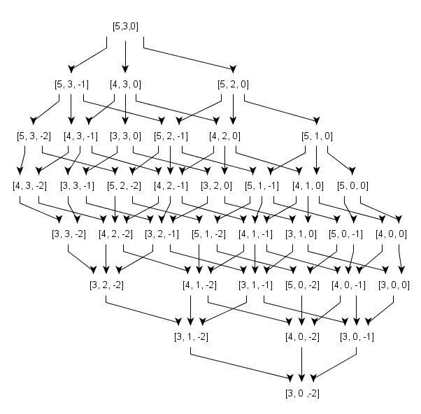
Figure 1. We use a graph to represent the rectangular prism corresponding to a finite dimensional representation $L((5,3,0))$ of $H_{\zeta}(\mathfrak{gl}_{3})$, with the highest weight of each $\mathfrak{gl}_{3}$ module indicated.

The decomposition of $L(\lambda)$ as a $\mathfrak{gl}_{n}$ module provides the character formula for $L(\lambda)$ as the sum of the characters of $\mathfrak{gl}_{n}$ modules:

(*) $$\chi_{\lambda;\zeta}=\sum_{0\leq\lambda-\lambda^{\prime}\leq\nu}\frac{\sum_{w\in S_{n}}(-1)^{w}e^{w(\lambda^{\prime}+\rho)}}{\sum_{w\in S_{n}}(-1)^{w}e^{w\rho}}.$$

As in the classical theory, this character allows us to calculate the decomposition of finite dimensional representations into irreducible ones.

Example 4.1.

Let us illustrate the decomposition of $L(\lambda)$ from the proof of Theorem 4.1; for clarity, we will work with $\mathfrak{sl}_{2}$ representations instead of $\mathfrak{gl}_{2}$ representations. Using the notation of the proof, $S_{k}=S^{k}(x_{1},x_{2})\cong V_{k}$, the irreducible $\mathfrak{sl}_{2}$ representation of dimension $k+1$. By the Clebsch-Gordon formula,

$$V_{m}\otimes V_{k}\cong V_{m+k}\oplus V_{m+k-2}\oplus\cdots\oplus V_{m+k-2\min(k,m)}.$$

We can use the above formula to draw the graph, as in Figure 2, representing the decomposition of $L((2,0))$, with $\nu=(0,3)$, into $\mathfrak{sl}_{2}$ modules. This representation is the quotient of $M((2,0))/H_{\zeta}(\mathfrak{gl}_{2})e_{21}^{3}v_{\lambda}$ by the submodules represented by the shaded areas of the diagram, and $L((2,0))\cong V_{2}\oplus V_{3}\oplus V_{4}\oplus V_{5}$ as $\mathfrak{sl}_{2}$ modules.

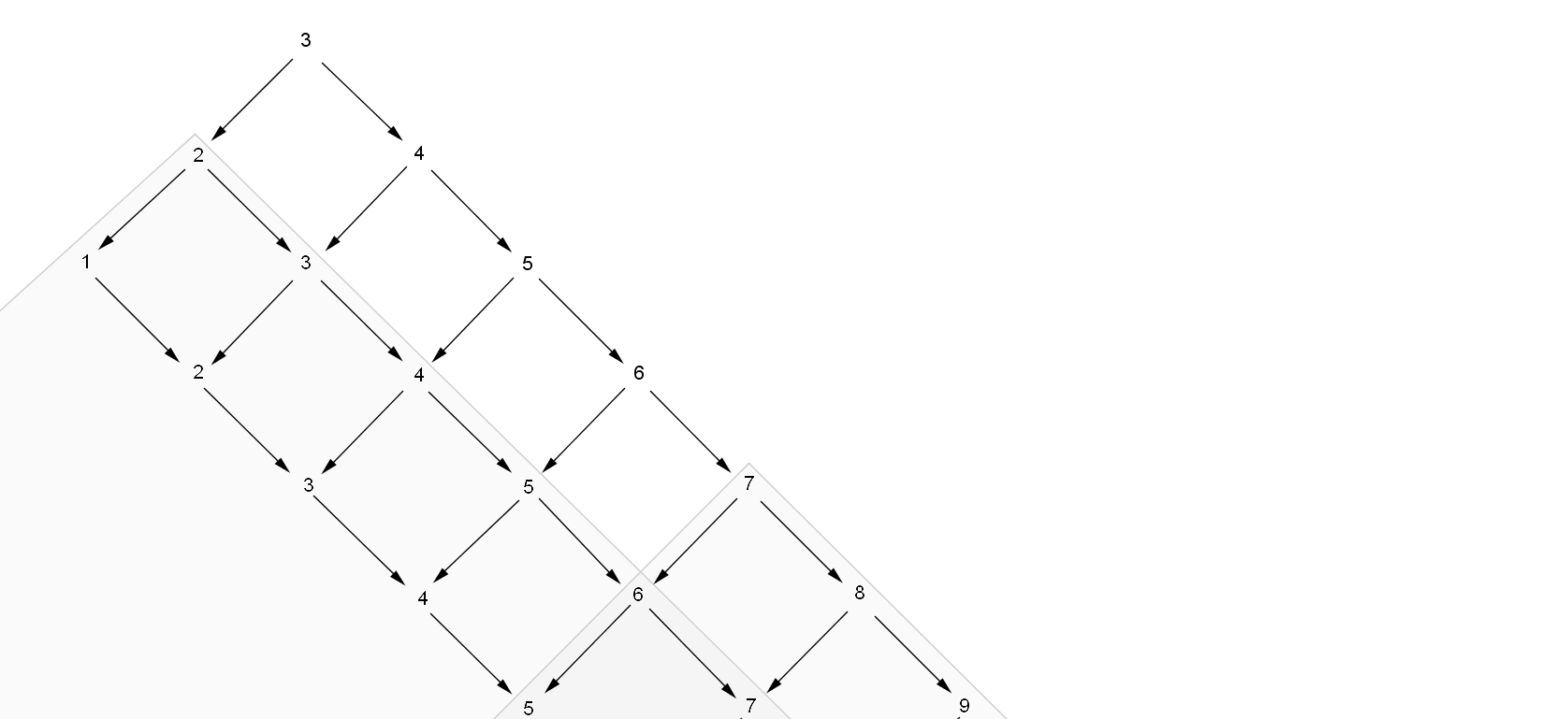
Figure 2. The decomposition of $L((2,0))$, with $\nu=(0,3)$, into $\mathfrak{sl}_{2}$ modules.

Example 4.2.

For $H_{\zeta}(\mathfrak{gl}_{1})$, the irreducible finite dimensional representation $L(\lambda)$, for $\lambda\in\mathbb{C}$, has character $\chi_{\lambda,\zeta}=\sum_{\nu^{\prime}=0}^{\nu}e^{\lambda-\nu^{\prime}}$, where $\nu$ is some nonnegative integer. If we describe $H_{\zeta}(\mathfrak{gl}_{1})$ as in Example 1.1, we can easily calculate the Casimir element to be $fe+g(h)$, where $g$ satisfies the equation $g(x)-g(x-1)=\phi(x)$. Then, $\nu$ is the smallest nonnegative integer such that $g(\lambda)-g(\lambda-\nu-1)=0$.

Example 4.3.

For $H_{\zeta}(\mathfrak{gl}_{2})$, the irreducible finite dimensional representations are necessarily of the form $L(\lambda)$ with $\lambda=(\lambda_{2}+m,\lambda_{2})$, where $\lambda_{2}\in\mathbb{C},\ m\in\mathbb{N}_{0}$. The character of $L(\lambda)$ equals

$$\chi_{\lambda;\zeta}=\sum_{(0,0)\leq(\nu_{1}^{\prime},\nu_{2}^{\prime})\leq(\nu_{1},\nu_{2})}\frac{e^{(\lambda_{2}+m-\nu_{1}^{\prime},\lambda_{2}-\nu_{2}^{\prime})}-e^{(\lambda_{2}-\nu_{2}^{\prime}-1,\lambda_{2}+m-\nu_{1}^{\prime}+1)}}{1-e^{(-1,1)}}.$$

Let $f_{1}(\lambda,\mu)=P(\lambda_{2}+m+\frac{1}{2},\lambda_{2}-\frac{1}{2})-P(\lambda_{2}+m+\frac{1}{2}-\mu,\lambda_{2}-\frac{1}{2})$ and $f_{2}(\lambda,\mu)=P(\lambda_{2}+m+\frac{1}{2},\lambda_{2}-\frac{1}{2})-P(\lambda_{2}+m+\frac{1}{2},\lambda_{2}-\mu-\frac{1}{2})$. Again, $\nu_{2}$ is defined as the minimal nonnegative integer satisfying $f_{2}(\lambda,\nu_{2}+1)=0$, while $\nu_{1}$ is either $m$ or the minimal nonnegative integer satisfying $f_{1}(\lambda,\nu_{1}+1)=0$. For instance, if $\zeta=\zeta_{0}r_{0}$ with $\zeta_{0}\neq 0$, then $f_{2}(\lambda,\mu)$ is a multiple of $\mu$, and so the only solution to the equation $f_{2}(\lambda,\nu_{2}+1)=0$ is $\nu_{2}=-1$, which is negative. Thus, $H_{\zeta_{0}r_{0}}(\mathfrak{gl}_{2})$ has no finite dimensional irreducible representations. If $\zeta=\zeta_{0}r_{0}+\zeta_{1}r_{1}$ with $\zeta_{1}\neq 0$, $P(\lambda)=\zeta_{0}(\lambda_{1}+\lambda_{2})+\zeta_{1}((\lambda_{1}+\frac{1}{2})^{2}+(\lambda_{1}+\frac{1}{2})(\lambda_{2}-\frac{1}{2})+(\lambda_{2}-\frac{1}{2})^{2})$, so $f_{2}(\lambda,\mu)=\zeta_{1}\mu\left(\frac{\zeta_{0}}{\zeta_{1}}+\lambda_{1}+2\lambda_{2}-\mu\right)$. Thus, $L(\lambda)$ is finite dimensional if and only if $\frac{\zeta_{0}}{\zeta_{1}}+\lambda_{1}+2\lambda_{2}$ is a positive integer. This agrees with the description of finite dimensional representations of $\mathfrak{sl}_{3}$.

4.2. Existence of $L(\lambda)$ with a given shape

Theorem 4.2.

For any $\mathfrak{gl}_{n}$ dominant weight $\lambda$ and $\nu\in\mathbb{N}_{0}^{n}$ such that $\nu_{i}\leq\lambda_{i}-\lambda_{i+1}$ for all $1\leq i\leq n-1$, there exists a deformation $\zeta$, such that the irreducible representation $L(\lambda)$ of $H_{\zeta}(\mathfrak{gl}_{n})$ is finite dimensional and its character is given by (*).

Proof.

Let $\lambda^{\prime}=\lambda+\rho$. We can write $\lambda^{\prime}_{i}=\lambda^{\prime}_{n}+k_{i}$ for $k_{1}>k_{2}>k_{3}>\cdots>k_{n-1}>k_{n}=0$ (we have strict inequalities because of the shift by $\rho$). Recall that $P(\lambda)=\sum w_{m}H_{m}(\lambda^{\prime})$ for $w_{i}$ defined as in Theorem 3.2. Let $\mu_{i}=(0,\ldots,\nu_{i}+1,0,\ldots,0)$. We will find $w_{i}$ such that $P(\lambda^{\prime})-P(\lambda^{\prime}-\mu_{i})=0$, while for all $0<\mu_{i}^{\prime}<\mu_{i}$, $P(\lambda^{\prime})-P(\lambda^{\prime}-\mu_{i}^{\prime})\neq 0$. This implies that there are embeddings of $M(\lambda^{\prime}-\mu_{i})$ into $M(\lambda^{\prime})$ with an irreducible quotient $L(\lambda^{\prime})=M(\lambda^{\prime})/\sum_{i}M(\lambda^{\prime}-\mu_{i})$, due to Theorem 4.1.

Define $P_{mj}=P(\lambda^{\prime})-P(\lambda^{\prime}-\mu)$ for $\mu=(0,\ldots,m+1,0,\ldots,0)$ with the $m+1$ at the $j$-th location. We must prove that there exist $w$ such that $P_{\nu_{1}1}=\cdots=P_{\nu_{n}n}=0$ and $P_{\nu_{1}^{\prime}1},\ldots,P_{\nu_{n}^{\prime}n}\neq 0$ for all $0<\nu_{i}^{\prime}<\nu_{i}$. We can write $P_{mj}=\sum_{i>0}w_{i}R_{mj}^{i}$, where

$$R_{mj}^{N}=\sum_{i_{1}+\ldots+i_{n}=N}(\lambda^{\prime}_{n}+k_{1})^{i_{1}}\cdots(\lambda^{\prime}_{n}+k_{j-1})^{i_{j-1}}((\lambda^{\prime}_{n}+k_{j})^{i_{j}}-(\lambda^{\prime}_{n}+k_{j}-m-1)^{i_{j}})(\lambda^{\prime}_{n}+k_{j+1})^{i_{j+1}}\cdots(\lambda^{\prime}_{n}+k_{n})^{i_{n}}.$$

Note that the condition $P_{kj}=0$ determines a hyperplane $\Pi_{kj}$ in the space $(w_{0},w_{1},\ldots)$ ($\Pi_{kj}$ might in fact be the entire space, but the following argument would be unaffected). Hence, the intersection $\bigcap\Pi_{\nu_{j}j}$ belongs to the union $\bigcup_{j,0<\nu_{j}^{\prime}<\nu_{j}}\Pi_{\nu_{j}^{\prime},j}$ if and only if it belongs to some $\Pi_{\nu_{j}^{\prime},j}$. Thus, it suffices to show that $\{P_{\nu_{1}1},\ldots,P_{\nu_{n}n},P_{\nu_{l}^{\prime}l}\}$ are linearly independent as functions of $w_{i}$ for all $1\leq l\leq n$ and $0<\nu_{l}^{\prime}<\nu_{l}$. This condition of linear independence is satisfied if

$$\det\left(\begin{matrix}R_{\nu_{1}1}^{1}&R_{\nu_{1}1}^{2}&\cdots&R_{\nu_{1}1}^{n+1}\\ R_{\nu_{2}2}^{1}&R_{\nu_{2}2}^{2}&\cdots&R_{\nu_{2}2}^{n+1}\\ \vdots&\vdots&\ddots&\vdots\\ R_{\nu_{n}n}^{1}&R_{\nu_{n}n}^{2}&\cdots&R_{\nu_{n}n}^{n+1}\\ R_{\nu_{l}^{\prime}l}^{1}&R_{\nu_{l}^{\prime}l}^{2}&\cdots&R_{\nu_{l}^{\prime}l}^{n+1}\\ \end{matrix}\right)\neq 0.$$

Now we shall prove that using column transformations, we can reduce the above matrix to its evaluation at $\lambda^{\prime}_{n}=0$. We proceed by induction on the column number. The elements of the first column, $R_{mj}^{1}$, are of degree zero with respect to $\lambda^{\prime}_{n}$, so $R_{mj}^{1}=R_{mj}^{1}(0)$. Suppose that using column transformations, all columns before column $p$ are reduced to their constant terms. Now, we note that

$$\frac{\partial R_{mj}^{p}(\lambda_{n}^{\prime})}{\partial\lambda^{\prime}_{n}} =\frac{\partial}{\partial\lambda^{\prime}_{n}}\left(\sum_{i_{1}+\ldots+i_{n}=p}(\lambda_{n}^{\prime}+k_{1})^{i_{1}}\cdots((\lambda_{n}^{\prime}+k_{j})^{i_{j}}-(\lambda_{n}^{\prime}+k_{j}-m-1)^{i_{j}})\cdots\lambda_{n}^{\prime i_{n}}\right)$$

$$=\sum_{i_{1}+\ldots+i_{n}=p-1}(i_{1}+i_{2}+\ldots+i_{n}+n)(\lambda_{n}^{\prime}+k_{1})^{i_{1}}\cdots((\lambda_{n}^{\prime}+k_{j})^{i_{j}}-(\lambda_{n}^{\prime}+k_{j}-m-1)^{i_{j}})\cdots\lambda_{n}^{\prime i_{n}}$$

$$=(p+n-1)R_{mj}^{p-1}(\lambda_{n}^{\prime}).$$

Thus, we see that $R_{mj}^{p}-R_{mj}^{p}(0)$ is a linear combination of $R_{mj}^{p-i}(0)$, the entries of the other columns:

$$R_{mj}^{p}(\lambda_{n}^{\prime})=\sum_{i}\frac{1}{i!}\lambda_{n}^{\prime i}\left.\frac{\partial^{i}R_{mj}^{p}}{\partial\lambda_{n}^{\prime i}}\right|_{\lambda^{\prime}_{n}=0}=\sum_{i}\frac{(p+n-1)\cdots(p+n-i)}{i!}\lambda_{n}^{\prime i}R_{mj}^{p-i}(0)=\sum_{i}{{p+n-1}\choose i}R_{mj}^{p-i}(0)\lambda_{n}^{\prime i}.$$

By selecting pivots of ${{p+n-1}\choose i}\lambda_{n}^{\prime i}$, we can eliminate every term except $R_{mj}^{p}(0)$. By repeating this step, we reduce the matrix to its evaluation at $\lambda^{\prime}_{n}=0$:

$$\det\left(\begin{matrix}R_{\nu_{1}1}^{1}(\lambda_{n}^{\prime})&R_{\nu_{1}1}^{2}(\lambda_{n}^{\prime})&\cdots&R_{\nu_{1}1}^{n+1}(\lambda_{n}^{\prime})\\ R_{\nu_{2}2}^{1}(\lambda_{n}^{\prime})&R_{\nu_{2}2}^{2}(\lambda_{n}^{\prime})&\cdots&R_{\nu_{2}2}^{n+1}(\lambda_{n}^{\prime})\\ \vdots&\vdots&\ddots&\vdots\\ R_{\nu_{n}n}^{1}(\lambda_{n}^{\prime})&R_{\nu_{n}n}^{2}(\lambda_{n}^{\prime})&\cdots&R_{\nu_{n}n}^{n+1}(\lambda_{n}^{\prime})\\ R_{\nu_{l}^{\prime}l}^{1}(\lambda_{n}^{\prime})&R_{\nu_{l}^{\prime}l}^{2}(\lambda_{n}^{\prime})&\cdots&R_{\nu_{l}^{\prime}l}^{n+1}(\lambda_{n}^{\prime})\\ \end{matrix}\right)=\det\left(\begin{matrix}R_{\nu_{1}1}^{1}(0)&R_{\nu_{1}1}^{2}(0)&\cdots&R_{\nu_{1}1}^{n+1}(0)\\ R_{\nu_{2}2}^{1}(0)&R_{\nu_{2}2}^{2}(0)&\cdots&R_{\nu_{2}2}^{n+1}(0)\\ \vdots&\vdots&\ddots&\vdots\\ R_{\nu_{n}n}^{1}(0)&R_{\nu_{n}n}^{2}(0)&\cdots&R_{\nu_{n}n}^{n+1}(0)\\ R_{\nu_{l}^{\prime}l}^{1}(0)&R_{\nu_{l}^{\prime}l}^{2}(0)&\cdots&R_{\nu_{l}^{\prime}l}^{n+1}(0)\\ \end{matrix}\right).$$

Let us now rewrite $R_{mj}^{N}(0)$:

$$R_{mj}^{N}(0) =\sum_{i_{1}+\ldots+i_{n}=N}k_{1}^{i_{1}}\cdots k_{j-1}^{i_{j-1}}(k_{j}^{i_{j}}-(k_{j}-m-1)^{i_{j}})k_{j+1}^{i_{j+1}}\cdots k_{n}^{i_{n}}=\sum_{i=0}^{N-1}H_{N-i-1}^{\prime}\left(k_{j}^{i+1}-(k_{j}-m-1)^{i+1}\right)$$

$$=\sum_{i=0}^{N-1}H_{N-i-1}\left(k_{j}^{i+1}-(k_{j}-m-1)^{i+1}-k_{j}(k_{j}^{i}-(k_{j}-m-1)^{i})\right)=\sum_{i=0}^{N-1}H_{N-i-1}\left((m+1)(k_{j}-m-1)^{i}\right)$$

where $H_{N-i}=\sum_{i_{1}+\ldots+i_{n}=N-i}k_{1}^{i_{1}}\cdots k_{n}^{i_{n}}$ and $H_{N-i}^{\prime}=\sum_{i_{1}+\ldots+\widehat{i_{j}}+\ldots+i_{n}=N-i}k_{1}^{i_{1}}\cdots\widehat{k_{j}^{i_{j}}}\cdots k_{n}^{i_{n}}$. The third equality is because $H_{N-i}^{\prime}=H_{N-i}-k_{j}H_{N-i-1}$. It is easy to see that the above determinant can be reduced further to

$$\det\left(\begin{matrix}\nu_{1}+1&(\nu_{1}+1)(k_{1}-\nu_{1}-1)&\cdots&(\nu_{1}+1)(k_{1}-\nu_{1}-1)^{n}\\ \nu_{2}+1&(\nu_{2}+1)(k_{2}-\nu_{2}-1)&\cdots&(\nu_{2}+1)(k_{2}-\nu_{2}-1)^{n}\\ \vdots&\vdots&\ddots&\cdots\\ \nu_{n}+1&(\nu_{n}+1)(k_{n}-\nu_{n}-1)&\cdots&(\nu_{n}+1)(k_{n}-\nu_{n}-1)^{n}\\ \nu_{l}^{\prime}+1&(\nu_{l}^{\prime}+1)(k_{l}-\nu_{l}^{\prime}-1)&\cdots&(\nu_{l}^{\prime}+1)(k_{l}-\nu_{l}^{\prime}-1)^{n}\\ \end{matrix}\right)=T\cdot\det\left(\begin{matrix}1&k_{1}-\nu_{1}-1&\cdots&(k_{1}-\nu_{1}-1)^{n}\\ 1&k_{2}-\nu_{2}-1&\cdots&(k_{2}-\nu_{2}-1)^{n}\\ \vdots&\vdots&\ddots&\cdots\\ 1&k_{n}-\nu_{n}-1&\cdots&(k_{n}-\nu_{n}-1)^{n}\\ 1&k_{l}-\nu_{l}^{\prime}-1&\cdots&(k_{l}-\nu_{l}^{\prime}-1)^{n}\\ \end{matrix}\right),$$

where $T=(\nu_{1}+1)(\nu_{2}+1)\cdots(\nu_{n}+1)(\nu_{l}^{\prime}+1)$ and the determinant is $\prod_{i=1}^{n}(k_{l}-k_{i}+\nu_{i}-\nu_{l}^{\prime})\prod_{1\leq i<j\leq n}(k_{j}-k_{i}+\nu_{i}-\nu_{j})$ by the Vandermonde determinant formula. Now, recalling the conditions $0\leq\nu_{i}\leq\lambda_{i}-\lambda_{i+1}=k_{i}-k_{i+1}-1$ we get $k_{j}-k_{i}+\nu_{i}-\nu_{j}<0$ for any $i<j$ and so $\prod_{1\leq i<j\leq n}(k_{j}-k_{i}+\nu_{i}-\nu_{j})$ is nonzero. Similarly, we get $\prod_{i=1}^{n}(k_{l}-k_{i}+\nu_{i}-\nu_{l}^{\prime})\neq 0$. Hence, the determinant is nonzero, and so $\{P_{\nu_{1},1},\ldots,P_{\nu_{n},n},P_{\nu_{l}^{\prime},l}\}$ are linearly independent as desired. ∎

  

5. Poisson Infinitesimal Cherednik Algebras

Now we will study infinitesimal Cherednik algebras by using their Poisson analogues. The Poisson infinitesimal Cherednik algebras are as natural as $H_{\zeta}(\mathfrak{gl}_{n})$, and their theory goes along the same lines with some simplifications. Although these algebras have not been defined before in the literature, the authors of [EGG] were aware of them, and technical calculations with these algebras are similar to those made in [T1]. This approach provides another proof of Theorem 3.1.

Let $\zeta$ be a deformation parameter, $\zeta:V\times V^{*}\to S(\mathfrak{gl}_{n})$. The Poisson infinitesimal Cherednik algebra $H_{\zeta}^{\prime}(\mathfrak{gl}_{n})$ is defined to be the algebra $S\mathfrak{gl}_{n}\otimes S(V\oplus V^{*})$ with a bracket defined on the generators by:

$$\{a,b\} =[a,b]\text{ for }a,b\in\mathfrak{gl}_{n},$$

$$\{g,v\} =g(v)\text{ for }g\in\mathfrak{gl}_{n},v\in V\oplus V^{*},$$

$$\{y,y^{\prime}\} =\{x,x^{\prime}\}=0\text{ for }y,y^{\prime}\in V,x,x^{\prime}\in V^{*},$$

$$\{y,x\} =\zeta(y,x)\text{ for }y\in V,x\in V^{*}.$$

This bracket extends to a Poisson bracket on $H_{\zeta}^{\prime}(\mathfrak{gl}_{n})$ if and only if the Jacobi identity $\{\{x,y\},z\}+\{\{y,z\},x\}+\{\{z,x\},y\}=0$ holds for any $x,y,z\in\mathfrak{gl}_{n}\ltimes(V\oplus V^{*})$. As can be verified by computations analogous to [EGG], Theorem 4.2, the Jacobi identiy holds iff $\zeta=\sum_{j=0}^{k}\zeta_{j}\mathfrak{r}_{j}$ where $\zeta_{j}\in\mathbb{C}$ and $\mathfrak{r}_{j}$ is the coefficient of $\tau^{j}$ in the expansion of $(x,(1-\tau A)^{-1}y)\det(1-\tau A)^{-1}$. Actually, we can consider the infinitesimal Cherednik algebras of $\mathfrak{gl}_{n}$ as quantizations of $H_{\zeta}^{\prime}(\mathfrak{gl}_{n})$.

Remark 5.1 (Due to Pavel Etingof).

Note that

$$\{y_{i},x_{j}\}=\sum\zeta_{l}\mathfrak{r}_{l}(y_{i},x_{j})=\sum\zeta_{l}\frac{\partial\operatorname{tr}(S^{l+1}A)}{\partial e_{ji}};$$

this follows from

$$\frac{\partial}{\partial B}(\det(1-\tau A)^{-1})=\frac{\operatorname{tr}(\tau B(1-\tau A)^{-1})}{\det(1-\tau A)}$$

when $B=y_{i}\otimes x_{j}$. In fact, if $\{y_{i},x_{j}\}=F_{ji}(A)$, the Jacobi identity implies that $F_{ij}(A)=\frac{\partial F}{\partial e_{ij}}$ for some $GL(n)$ invariant function $F$, and that $\Lambda^{2}D_{A}(F)=0$, where $D_{A}$ is the matrix with $(D_{A})_{{}_{ij}}=\frac{\partial}{\partial e_{ij}}$. One can then show that the only $GL(n)$ invariant functions $F$ satisfying this partial differential equation are linear combinations of $\operatorname{tr}(S^{l}A)$.

Our main goal is to compute explicitly the Poisson center of the algebra $H_{\zeta}^{\prime}(\mathfrak{gl}_{n})$. As before, we set $\mathcal{Q}_{k}$ to be the coefficient of $(-t)^{k}$ in the expansion of $\det(1-tA)$, $\tau_{k}=\sum_{i=1}^{n}x_{i}\{\mathcal{Q}_{k},y_{i}\}$, and $\zeta(z)=\zeta_{0}+\zeta_{1}z+\zeta_{2}z^{2}+\cdots$.

Theorem 5.1.

The Poisson center $\operatorname{\mathfrak{z}_{\mathrm{Pois}}}(H_{\zeta}^{\prime}(\mathfrak{gl}_{n}))=\mathbb{C}[\tau_{1}+c_{1},\tau_{2}+c_{2},\ldots,\tau_{n}+c_{n}]$, where $(-1)^{i}c_{i}$ is the coefficient of $t^{i}$ in the series

$$c(t)=\operatorname{Res}_{z=0}\zeta(z^{-1})\frac{\det(1-tA)}{\det(1-zA)}\frac{1}{1-t^{-1}z}\frac{dz}{z}.$$

Proof.

First, we claim that $\operatorname{\mathfrak{z}_{\mathrm{Pois}}}(H_{0}^{\prime}(\mathfrak{gl}_{n}))=\mathbb{C}[\tau_{1},\ldots,\tau_{n}]$. The inclusion $\mathbb{C}[\tau_{1},\ldots,\tau_{n}]\subseteq\operatorname{\mathfrak{z}_{\mathrm{Pois}}}(H_{0}^{\prime}(\mathfrak{gl}_{n}))$ is straightforward, while the reverse inclusion follows from the structure of the coadjoint action of the Lie group corresponding to $\mathfrak{gl}_{n}\ltimes(V\oplus V^{*})$ (as in the proof of [T1], Theorem 2).

We prove that the Poisson center of $H_{0}^{\prime}(\mathfrak{gl}_{n})$ can be lifted to the Poisson center of $H_{\zeta}^{\prime}(\mathfrak{gl}_{n})$ by verifying that $\tau_{i}+c_{i}$ are indeed Poisson central. Since $\tau_{k}\in\operatorname{\mathfrak{z}_{\mathrm{Pois}}}(H_{0}(\mathfrak{gl}_{n}))$ and $c_{k}\in\operatorname{\mathfrak{z}_{\mathrm{Pois}}}(S(\mathfrak{gl_{n}}))$, $\tau_{k}+c_{k}$ Poisson-commutes with elements of $S(\mathfrak{gl}_{n})$. We can define an anti-involution on $H_{\zeta}^{\prime}(\mathfrak{gl}_{n})$ that acts on basis elements by taking $e_{ij}$ to $e_{ji}$ and $y_{i}$ to $x_{i}$. By using the arguments explained in the proof of Theorem 2 in [T1], we can show that $\tau_{k}$ is fixed by this anti-involution, while $c_{k}$ is also fixed since it lies in $\operatorname{\mathfrak{z}_{\mathrm{Pois}}}(S(\mathfrak{gl_{n}}))$. Applying this anti-involution, we see that it suffices to show that $c_{k}$ satisfies $\{\tau_{k}+c_{k},y_{l}\}=0$ for basis elements $y_{l}\in V$.

First, notice that if $g\in S(\mathfrak{gl}_{n})$, then $\{g,y_{l}\}=\sum_{i,j=1}^{n}\frac{\partial g}{\partial e_{ij}}\{e_{ij},y_{l}\}$, and together with the equation $\{\{\mathcal{Q}_{k},y_{i}\},y_{l}\}=0$ (see the proof of Lemma 2.1 in [T1]), we get

$$\{\tau_{k},y_{l}\}=\left\{\sum_{i=1}^{n}x_{i}\{\mathcal{Q}_{k},y_{i}\},y_{l}\right\}=\sum_{i=1}^{n}\{x_{i},y_{l}\}\{\mathcal{Q}_{k},y_{i}\}=-\sum_{i=1}^{n}\left(\operatorname{Res}_{z=0}\zeta(z^{-1})\frac{\operatorname{tr}(x_{i}(1-zA)^{-1}y_{l})}{z\det(1-zA)}dz\right)\{\mathcal{Q}_{k},y_{i}\}.$$

Thus, we have

$$\{\tau_{k}+c_{k},y_{l}\}=\sum_{i,j=1}^{n}\frac{\partial c_{k}}{\partial e_{ij}}\{e_{ij},y_{l}\}-\sum_{i=1}^{n}\left(\operatorname{Res}_{z=0}\zeta(z^{-1})\frac{\operatorname{tr}(x_{i}(1-zA)^{-1}y_{l})}{z\det(1-zA)}dz\right)\{\mathcal{Q}_{k},y_{i}\}.$$

Hence, $\{\tau_{k}+c_{k},y_{l}\}=0$ is equivalent to the system of partial differential equations:

$$\sum_{i,j=1}^{n}\frac{\partial c_{k}}{\partial e_{ij}}\{e_{ij},y_{l}\}=\sum_{i=1}^{n}\left(\operatorname{Res}_{z=0}\zeta(z^{-1})\frac{\operatorname{tr}(x_{i}(1-zA)^{-1}y_{l})}{z\det(1-zA)}dz\right)\{\mathcal{Q}_{k},y_{i}\}.$$

Multiplying both sides by $(-t)^{k}$ and summing over $k=1,\ldots,n,$ we obtain an equivalent single equation

$$\sum_{i,j=1}^{n}\frac{\partial c(t)}{\partial e_{ij}}\{e_{ij},y_{l}\}=\sum_{i=1}^{n}\left(\operatorname{Res}_{z=0}\zeta(z^{-1})\frac{\operatorname{tr}(x_{i}(1-zA)^{-1}y_{l})}{z\det(1-zA)}dz\right)\{\det(1-tA),y_{i}\}.$$

Since all terms above are $GL(n)$ invariant and diagonalizable matrices are dense in $\mathfrak{gl}_{n}$, we can set $A=\mathrm{diag}(a_{1},\ldots,a_{n})$:

$$\frac{\partial c(t)}{\partial a_{l}}y_{l} =\left(\operatorname{Res}_{z=0}\frac{\zeta(z^{-1})}{z(1-za_{l})\det(1-zA)}dz\right)\{\det(1-tA),y_{l}\}$$

$$=\left(\operatorname{Res}_{z=0}\frac{\zeta(z^{-1})}{z(1-za_{l})\det(1-zA)}dz\right)\frac{\partial\det(1-tA)}{\partial a_{l}}y_{l}$$

$$=-\left(\operatorname{Res}_{z=0}\frac{\zeta(z^{-1})}{z(1-za_{l})\det(1-zA)}dz\right)\frac{t\det(1-tA)}{1-ta_{l}}y_{l},$$

and it is easy to see that $c(t)$ satisfies the above equation. ∎

Example 5.1.

In particular, $c_{1}=\sum_{i=0}^{k}\zeta_{i}\operatorname{tr}S^{i+1}A$.

Remark 5.2.

Another way of writing the formula for $c_{k}$ is

$$c_{k}=\operatorname{Res}_{z=0}\zeta(z^{-1})G_{k}(z)\frac{dz}{z^{2}},$$

where $G_{k}(z)=\sum z^{m}y_{m,k}(A)$ and $y_{m,k}(A)=\chi\underbrace{(m,1,\ldots,1)}_{k}$, the character of an irreducible $\mathfrak{gl}_{n}$ module corresponding to a hook Young diagram. This provides a better insight for the quantization construction.

Remark 5.3.

We expect that for any $a_{1},\ldots,a_{n}\in\mathbb{C}$, the induced symplectic structure on $\mathrm{Spec}(S(\mathfrak{gl}_{n})\otimes S(V\oplus V^{*})/(\tau_{1}+c_{1}-a_{1},\ldots,\tau_{n}+c_{n}-a_{n}))$ has only finitely many symplectic leaves.

  

6. Passing from Commutative to Noncommutative Algebras

Note that $\{g,y\}\in S(\mathfrak{gl}_{n})\otimes V$ for $g\in S(\mathfrak{gl}_{n})$ and $y\in V$; we can thus identify $\{g,y\}=\sum_{i=1}^{n}h_{i}\otimes y_{i}\in H_{\zeta}^{\prime}(\mathfrak{gl}_{n})$ with the element $\sum_{i=1}^{n}\mathrm{Sym}(h_{i})y_{i}\in H_{\zeta}(\mathfrak{gl}_{n})$.

Lemma 6.1.

$$[\operatorname{tr}S^{k+1}A,y]=\left\{\sum_{j=0}^{k}\frac{(-1)^{j}}{k+n+1}{k+n+1\choose j+1}\operatorname{tr}S^{k+1-j}A,y\right\}.$$

Proof.

It is enough to consider the case $y=y_{1}$. Recall that $\operatorname{tr}S^{k+1}(A)$ can be written as a sum of degree $k+1$ monomials of form $e_{1,i_{1}}\cdots e_{1,i_{s_{1}}}e_{2,i_{s_{1}+1}}\cdots e_{2,i_{s_{1}+s_{2}}}\cdots e_{n,i_{s_{1}+\cdots+s_{n}}}$ where $s_{1}+\cdots+s_{n}=k+1$ and the sequence $\{i_{k}\}$ is a permutation of the sequence of $s_{1}$ ones, $s_{2}$ twos, and so forth; for conciseness, we will denote the above monomial by $e_{1,i_{1}}\cdots e_{n,i_{k+1}}$. The only terms of $\operatorname{tr}S^{k+1}A$ that contribute to $[\operatorname{tr}S^{k+1}A,y_{1}]$ and to $\{\operatorname{tr}S^{k+1}A,y_{1}\}$ have $s_{1}\geq 1$. Since to compute $[\operatorname{tr}S^{k+1}A,y_{1}]$ we first symmetrize $\operatorname{tr}S^{k+1}A$, we will compute $[\mathrm{Sym}(e_{1,i_{1}}\cdots e_{n,i_{k+1}}),y_{1}]-\{\mathrm{Sym}(e_{1,i_{1}}\cdots e_{n,i_{k+1}}),y_{1}\}$. For both the Lie bracket and the Poisson bracket, we use Leibniz’s rule to compute the bracket, but whereas in the Poisson case we can transfer the resulting elements of $V$ to the right since the Poisson algebra is commutative, in the Lie case when we do so extra terms appear.

Consider a typical term that may appear after we use Leibniz’s rule to compute $[\operatorname{tr}S^{k+1}A,y_{1}]$:

$$\cdots y_{j_{0}}\cdots e_{j_{1}j_{0}}\cdots e_{j_{2}j_{1}}\cdots e_{j_{N}j_{N-1}}\cdots$$

When we move $y_{j_{0}}$ to the right, we get, besides $\cdots e_{j_{1}j_{0}}\cdots e_{j_{2}j_{1}}\cdots e_{j_{N}j_{N-1}}\cdots y_{j_{0}}$, additional residual terms like $-\cdots e_{j_{2}j_{1}}\cdots e_{j_{N}j_{N-1}}\cdots y_{j_{1}}$ and $\cdots e_{j_{3}j_{2}}\cdots e_{j_{N}j_{N-1}}\cdots y_{j_{2}}$, up to $(-1)^{N}\cdots y_{j_{N}}$. Without loss of generality, we can consider only the last expression, since the others will appear in the smaller chains

$$\cdots y_{j_{0}}\cdots e_{j_{1}j_{0}}\cdots\widehat{e_{j_{2}j_{1}}}\cdots\widehat{e_{j_{3}j_{2}}}\cdots\widehat{e_{j_{N}j_{N-1}}}$$

and

$$\cdots y_{j_{0}}\cdots e_{j_{1}j_{0}}\cdots e_{j_{2}j_{1}}\cdots\widehat{e_{j_{3}j_{2}}}\cdots\widehat{e_{j_{N}j_{N-1}}},$$

and so forth, with the same coefficients. For notational convenience, we let $z_{1}$ denote the coefficient of $y_{j_{N}}$ in the residual term, i.e., the term represented by the ellipsis: $(-1)^{N}\underbrace{\cdots}_{z_{1}}y_{j_{N}}$. Then, $z_{1}y_{j_{N}}$ is a term in the expression $(-1)^{N}\{z_{1}e_{j_{N}1},y_{1}\}$, which appears in $(-1)^{N}\{\operatorname{tr}S^{k+1-N}A,y_{1}\}$. Thus, we can write

$$[\operatorname{tr}S^{k+1}A,y_{1}]=\left\{\sum_{N=0}^{k}(-1)^{N}C_{N}\operatorname{tr}S^{k+1-N}A,y_{1}\right\}$$

for some coefficients $C_{N}$.

Next, we compute $C_{N}$. We first count how many times $z_{1}y_{j_{N}}$ appears in $\{\operatorname{tr}S^{k+1-N}A,y_{1}\}$. Notice that since $z_{1}$ is the product of $k-N$ $e_{jl}$’s, we can insert $e_{j_{N}1}$ in $k-N+1$ places to obtain $z_{2}$ such that $\{z_{2},y_{1}\}$ contains $z_{1}y_{j_{N}}$.

Now we compute the coefficient of $z_{2}$ in $\operatorname{tr}S^{k+1-N}A$. As noted before, $\operatorname{tr}S^{k+1-N}(A)$ can be written as a sum of degree $k+1-N$ monomials of form $e_{1,i_{1}}\cdots e_{1,i_{s_{1}}}e_{2,i_{s_{1}+1}}\cdots e_{2,i_{s_{1}+s_{2}}}\cdots e_{n,i_{k+1-N}}$. Any term that is a permutation of those $k+1-N$ unit matrices will appear in the symmetrization of $\operatorname{tr}S^{k+1-N}A$. We count the number of sequences $i_{1},\ldots,i_{k+1-N}$ such that $z_{2}$ is the product of the elements $e_{1,i_{1}},\ldots,e_{n,i_{k+1-N}}$ (in some order); this tells us the multiplicity of $z_{2}$ in the symmetrization of $\operatorname{tr}S^{k+1-N}A$. Suppose $z_{2}=e_{1,i_{1}}\cdots e_{n,i_{k+1-N}}$ for a certain sequence $i_{1},\ldots,i_{k+1-N}$. Then, $z_{2}=e_{1,i_{1}^{\prime}}\cdots e_{n,i_{k+1-N}^{\prime}}$ if and only if $i_{s_{1}+\cdots+s_{j-1}+1}^{\prime},\ldots,i_{s_{1}+\cdots+s_{j}}^{\prime}$ is a permutation of $i_{s_{1}+\cdots+s_{j-1}+1},\ldots,i_{s_{1}+\cdots+s_{j}}$ for all $j$. Thus, $z_{2}$ appears $s_{1}!s_{2}!\cdots s_{n}!$ times in $\operatorname{tr}S^{k+1-N}A$. Since each term has coefficient $\frac{1}{(k-N+1)!}$ in the symmetrization, $z_{2}$ appears with coefficient

$$\frac{s_{1}!s_{2}!\cdots s_{n}!}{(k-N+1)!}$$

in the symmetrization of $\operatorname{tr}S^{k+1-N}A$. In conjunction with the previous paragraph, we see that $z_{1}y_{j_{N}}$ appears

$$\frac{s_{1}!s_{2}!\cdots s_{n}!}{(k-N+1)!}\times(k-N+1)=\frac{s_{1}!s_{2}!\cdots s_{n}!}{(k-N)!}$$

times in $\{\operatorname{tr}S^{k+1-N}A,y_{1}\}$.

It remains to calculate how many times $z_{1}y_{j_{N}}$ appears in $[\operatorname{tr}S^{k+1}A,y_{1}]$. Recall that $z_{1}$ is obtained from a term like:

$$\cdots e_{j_{0}1}\cdots e_{j_{1}j_{0}}\cdots e_{j_{2}j_{1}}\cdots e_{j_{N}j_{N-1}}\cdots$$

where the ordered union of the ellipsis equals $z_{1}$. Thus, $z_{1}$ comes from terms of the following form: we choose arbitrary numbers $j_{0},\ldots,j_{N-1}$, and insert $e_{j_{0}1},e_{j_{1}j_{0}},\ldots,e_{j_{N}j_{N-1}}$ into $z_{1}$. There are

$$\frac{(k+1)(k)\cdots(k+1-N)}{(N+1)!}$$

ways for this choice for any fixed $j_{0},\ldots,j_{N-1}$. Any such term $z_{3}$ appears in $\operatorname{tr}S^{k+1}A$ with coefficient

$$\frac{s_{1}^{\prime}!\cdots s_{n}^{\prime}!}{(k+1)!}$$

where $s_{l}^{\prime}$ is the total number of $e_{li}$’s (for some $i$) in $z_{3}$, i.e., $s_{l}+\text{number of }j_{i}\text{'s with }j_{i}=l$, $0\leq i<N$.

Combining the results of the last two paragraphs, we see that $\{\operatorname{tr}S^{k+1-N}A,y_{1}\}$ must appear with coefficient

$$\left(\frac{(k+1)(k)\cdots(k+1-N)}{(N+1)!}\sum\frac{s_{1}^{\prime}!\cdots s_{n}^{\prime}!}{(k+1)!}\right)\left.\middle/\frac{s_{1}!s_{2}!\cdots s_{n}!}{(k-N)!}\right.=\frac{1}{(N+1)!}\sum\frac{s_{1}^{\prime}!\cdots s_{n}^{\prime}!}{s_{1}!s_{2}!\cdots s_{n}!},$$

where the summation is over all length-$N$ sequences $\{j_{l}\}$ of integers from 1 to $n$. We claim that

$$\frac{\sum s_{1}^{\prime}!\cdots s_{n}^{\prime}!}{s_{1}!\cdots s_{n}!}=(k+n)\cdots(k+n-N+1).$$

To see this, notice that $\frac{\sum s_{1}^{\prime}!\cdots s_{n}^{\prime}!}{s_{1}!\cdots s_{n}!}$ is the coefficient of $t^{N}$ in the expression

$$N!\prod_{i=1}^{n}\left(1+(s_{i}+1)t+\frac{(s_{i}+1)(s_{i}+2)}{2!}t^{2}+\cdots\right).$$

The above generating function equals $N!\prod_{i=1}^{n}(1-t)^{-(s_{i}+1)}=N!(1-t)^{-(k+1-N+n)}$, and the coefficient of $t^{N}$ in this expression is $(k+n)\cdots(k+n-N+1)$.

Finally, we arrive at the simplified coefficient of $\{\operatorname{tr}S^{k+1-N}A,y_{1}\}$:

$$C_{N}=\frac{1}{(N+1)!}\sum\frac{s_{1}^{\prime}!\cdots s_{n}^{\prime}!}{s_{1}!s_{2}!\cdots s_{n}!}=\frac{(k+n)\cdots(k+n-N+1)}{(N+1)!},$$

as desired. ∎

Now we will give an alternative proof of Theorem 3.1.

Proof.

Let $f(z)$ be the polynomial satisfying $f(z)-f(z-1)=\partial^{n}(z^{n}\zeta(z))$ and $g(z)=z^{1-n}\frac{1}{\partial^{n-1}}f(z)$ (in the expression for $g(z)$, we discard any negative powers of $z$). Note that if $g(z)=g_{k+1}z^{k+1}+\cdots+g_{1}z$, then

$$\zeta(z)=\sum_{j=1}^{k+1}\sum_{i=0}^{j-1}\frac{1}{j+n}{j+n\choose i+1}(-1)^{i}g_{j}z^{j-1-i},\ \ \ \zeta_{j-1}=\sum_{i=0}^{k-j+1}\frac{1}{j+i+n}{j+n+i\choose i+1}(-1)^{i}g_{j+i}.$$

Lemma 6.1 allows us to write

$$\left[\sum_{j=1}^{k+1}g_{j}\operatorname{tr}S^{j}A,y\right] =\left\{\sum_{j=1}^{k+1}\sum_{i=0}^{j-1}\frac{1}{j+n}{j+n\choose i+1}(-1)^{i}g_{j}\operatorname{tr}S^{j-i}A,y\right\}$$

$$=\left\{\sum_{j=1}^{k+1}\sum_{i=0}^{k-j+1}\frac{1}{j+i+n}{j+i+n\choose i+1}(-1)^{i}g_{j+i}\operatorname{tr}S^{j}A,y\right\}=\left\{\sum_{j=1}^{k+1}\zeta_{j-1}\operatorname{tr}S^{j}A,y\right\}.$$

Hence,

$$[t_{1},y]=\sum_{i=1}^{n}[x_{i},y]y_{i}=\sum_{i=1}^{n}\{x_{i},y\}y_{i}=-\left\{\sum_{j=1}^{k+1}\zeta_{j-1}\operatorname{tr}S^{j}A,y\right\}=-\left[\sum_{j=1}^{k+1}g_{j}\operatorname{tr}S^{j}A,y\right],$$

where the third equality follows from the fact that $\tau_{1}+\sum_{j=1}^{k+1}\zeta_{j-1}\operatorname{tr}S^{j}A$ is Poisson-central in $H_{\zeta}^{\prime}(\mathfrak{gl}_{n})$ (see Example 5.1). Thus, we get $t_{1}^{\prime}=t_{1}+C^{\prime}$, where

$$C^{\prime}=\sum_{j=1}^{k+1}g_{j}\operatorname{tr}S^{j}A=\operatorname{Res}_{z=0}g(z^{-1})\det(1-zA)^{-1}z^{-1}dz.$$

∎

Remark 6.1.

Comparing the formula for $c_{1}$ in Example 5.1 to the one from Theorem 3.1, we see that they differ only by a change $z\zeta(z)\rightsquigarrow g(z)$. We expect that a similar twist of the formula for $c(t)$ given in Theorem 5.1 will provide the formulas for the actions of the generators of $\mathfrak{z}(H_{\zeta}(\mathfrak{gl}_{n}))$ on the Verma module $M(\lambda-\rho)$.

  

7. Algebras $H_{\zeta}(\mathfrak{sp}_{2n})$ and $H_{\zeta}^{\prime}(\mathfrak{sp}_{2n})$

Let $V$ be the standard $2n$-dimensional representation of $\mathfrak{sp}_{2n}$ with symplectic form $\omega$, and let $\zeta:V\times V\rightarrow U(\mathfrak{sp}_{2n})$ be an $\mathfrak{sp}_{2n}$ invariant bilinear form. The infinitesimal Cherednik algebra $H_{\zeta}(\mathfrak{sp}_{2n})$ is defined as the quotient of $U(\mathfrak{sp}_{2n})\ltimes T(V)$ by the relation $[x,y]=\zeta(x,y)$ for all $x,y\in V$, such that $H_{\zeta}(\mathfrak{sp}_{2n})$ satisfies the PBW property. In [EGG], Theorem 4.2, it was shown that $H_{\zeta}(\mathfrak{sp}_{2n})$ satisfies the PBW property if and only if $\zeta=\sum_{j=0}^{k}\zeta_{2j}r_{2j}$ where $r_{j}$ is the symmetrization of the coefficient of $z^{j}$ in the expansion of

$$\omega(x,(1-z^{2}A^{2})^{-1}y)\det(1-zA)^{-1}=r_{0}(x,y)+r_{2}(x,y)z^{2}+\cdots.$$

Note that for $A\in\mathfrak{sp}_{2n}$, the expansion of $\det(1-zA)^{-1}$ contains only even powers of $z$.

Remark 7.1.

For $\zeta_{0}\neq 0$, there is an isomorphism $H_{\zeta_{0}r_{0}}(\mathfrak{sp}_{2n})\cong U(\mathfrak{sp}_{2n})\ltimes A_{n}$, where $A_{n}$ is the $n$-th Weyl algebra (see [EGG] Example 4.11). Thus, we can regard $H_{\zeta}(\mathfrak{sp}_{2n})$ as a deformation of $U(\mathfrak{sp}_{2n})\ltimes A_{n}$.

Choose a basis $v_{j}$ of $V$, so that

$$\omega(x,y)=x^{T}Jy,$$

with

$$J=\left(\begin{matrix}0&1&0&0&\cdots&0&0\\ -1&0&0&0&\cdots&0&0\\ 0&0&0&1&\cdots&0&0\\ 0&0&-1&0&\ddots&\vdots&\vdots\\ \vdots&\vdots&\vdots&\ddots&\ddots&\vdots&\vdots\\ 0&0&0&0&\cdots&0&1\\ 0&0&0&0&\cdots&-1&0\end{matrix}\right).$$

As before, we study the noncommutative infinitesimal Cherednik algebra $H_{\zeta}(\mathfrak{sp}_{2n})$ by considering its Poisson analogue $H_{\zeta}^{\prime}(\mathfrak{sp}_{2n})$. We define $\sum_{i=0}^{n}\mathcal{Q}_{i}z^{2i}=\det(1-zA)$ and

$$\uptau_{i}=(-1)^{i-1}\sum_{j=1}^{2n}\{\mathcal{Q}_{i},v_{j}\}v_{j}^{*},$$

where $\{v_{j}^{*}\}$ is dual to $\{v_{j}\}$ (that is, $\omega(v_{i},v_{j}^{*})=\delta_{ij}$). When viewed as an element of $\mathbb{C}[\mathfrak{sp}_{2n}\ltimes V]$,

$$\uptau_{i}=-\sum_{j=0}^{i-1}\mathcal{Q}_{j}\omega(A^{2i-1-2j}v,v),$$

so $\uptau_{i}$ is $\mathfrak{sp}_{2n}$ invariant and independent of the choice of basis $\{v_{i}\}$.

Proposition 7.1.

The Poisson center of $H_{0}^{\prime}(\mathfrak{sp}_{2n})$ is $\mathbb{C}[\uptau_{1},\ldots,\uptau_{n}]$.

Proof.

We will follow a similar approach as in the proof of Theorem 2.1, [T1]. Let $L$ be the Lie algebra $\mathfrak{sp}_{2n}\ltimes V$ and $S$ be the Lie group of $L$. We need to verify that $\mathbb{C}[\uptau_{1},\ldots,\uptau_{n}]=\operatorname{\mathfrak{z}_{\mathrm{Pois}}}(H_{0}^{\prime}(\mathfrak{sp}_{2n}))$, the latter being identified with $\mathbb{C}[L^{*}]^{S}$. Let $M\subset L$ be the $2n$-dimensional subspace consisting of elements of the form

$$y=\left\{\left(\begin{matrix}0&y_{12}&0&\cdots&0&0\\ y_{21}&\ddots&\ddots&\ddots&\vdots&\vdots\\ 0&\ddots&0&y_{2n-3,2n-2}&0&0\\ 0&0&y_{2n-2,2n-3}&0&0&0\\ 0&\cdots&0&0&0&y_{2n-1,2n}\\ 0&\cdots&0&0&0&0\end{matrix}\right),\left(\begin{matrix}0\\ 0\\ \vdots\\ 0\\ 0\\ y_{2n}\end{matrix}\right)\right\},$$

where all the $y$’s belong to $\mathbb{C}$. In what follows, we identify $L^{*}$ and $L$ via the non-degenerate pairing, so that the coadjoint action of $S$ is on $L$. We use the following two facts proved in [K]: first, that the orbit of $M$ under the coadjoint action of $S$ on $L^{*}$ is dense in $L^{*}$; and second, that $\mathbb{C}[L^{*}]^{S}\cong\mathbb{C}[f_{1},\ldots,f_{n}]$, where

$$\left.f_{i}\right|_{M}(y)=\sigma_{i-1}(y_{2,1}y_{1,2},y_{3,2}y_{2,3},\ldots,y_{2n-2,2n-3}y_{2n-3,2n-2})y_{2n-1,2n}y_{2n}^{2}$$

and $\sigma_{j}$ is the $j$-th elementary symmetric polynomial. It is straightforward to see that $\left.\uptau_{i}\right|_{M}=f_{i}$, and so $\mathbb{C}[L^{*}]^{S}\cong\mathbb{C}[\uptau_{1},\ldots,\uptau_{n}]$ as desired. ∎

As before, let $\zeta(z)=\zeta_{0}+\zeta_{2}z^{2}+\zeta_{4}z^{4}+\cdots$.

Theorem 7.1.

The Poisson center $\operatorname{\mathfrak{z}_{\mathrm{Pois}}}(H_{\zeta}^{\prime}(\mathfrak{sp}_{2n}))=\mathbb{C}[\uptau_{1}+c_{1},\uptau_{2}+c_{2},\ldots,\uptau_{n}+c_{n}]$, where $(-1)^{i-1}c_{i}$ is the coefficient of $t^{2i}$ in the series

$$c(t)=2\operatorname{Res}_{z=0}\zeta(z^{-1})\frac{\det(1-tA)}{\det(1-zA)}\frac{z^{-1}}{1-z^{2}t^{-2}}dz.$$

Proof.

Since $c_{i}\in\operatorname{\mathfrak{z}_{\mathrm{Pois}}}(S(\mathfrak{sp}_{2n}))$, $\{\uptau_{i}+c_{i},g\}=0$ for any $g\in S(\mathfrak{sp}_{2n})$, and so it suffices to show that $\{\uptau_{i}+c_{i},v\}=0$ for all $v\in V$. By the Jacobi rule,

$$\{\uptau_{i},v\}=(-1)^{i-1}\sum_{j}\{\mathcal{Q}_{i},v_{j}\}\{v_{j}^{*},v\}+(-1)^{i-1}\sum_{j}\{\{\mathcal{Q}_{i},v_{j}\},v\}v_{j}^{*}.$$

Thus,

(1) $$\{\uptau_{i}+c_{i},v\}=(-1)^{i-1}\sum_{j}\{\mathcal{Q}_{i},v_{j}\}\{v_{j}^{*},v\}+(-1)^{i-1}\sum_{j}\{\{\mathcal{Q}_{i},v_{j}\},v\}v_{j}^{*}+\{c_{i},v\}.$$

In the case of $H_{\zeta}^{\prime}(\mathfrak{gl}_{n})$, $\sum_{j}\{\{\mathcal{Q}_{i},y_{j}\},y\}x_{j}=0$ by straightforward application of properties of the determinant. However, for $H_{\zeta}^{\prime}(\mathfrak{sp}_{2n})$, $\sum_{j}\{\{\mathcal{Q}_{i},v_{j}\},v\}v_{j}^{*}\neq 0$. To calculate this sum, let $B$ be a basis of $\mathfrak{sp}_{2n}$ (the basis elements are given in the Appendix, but for the purposes of this section, the specific elements are not needed). Write

$$\sum_{j}\{\{\mathcal{Q}_{i},v_{j}\},v\}v_{j}^{*}=\sum_{j}\left\{\sum_{e\in B}\frac{\partial\mathcal{Q}_{i}}{\partial e}e(v_{j}),v\right\}v_{j}^{*}=\sum_{j}\left(\sum_{e\in B}\frac{\partial\mathcal{Q}_{i}}{\partial e}\{e(v_{j}),v\}v_{j}^{*}+\left\{\frac{\partial\mathcal{Q}_{i}}{\partial e},v\right\}e(v_{j})v_{j}^{*}\right).$$

Lemma 7.1.

$$\sum_{j}\sum_{e\in B}\left\{\frac{\partial\mathcal{Q}_{i}}{\partial e},v\right\}e(v_{j})v_{j}^{*}=0.$$

The proof of this lemma is quite technical and is provided in the Appendix.

Using the fact that $\sum_{j}\{\{\mathcal{Q}_{i},v_{j}\},v\}v_{j}^{*}=\sum_{j}\sum_{e\in B}\frac{\partial\mathcal{Q}_{i}}{\partial e}\{e(v_{j}),v\}v_{j}^{*}$, we can restrict (1) to diagonal matrices, which are spanned by elements $e_{i}=\mathrm{diag}(0,\ldots,1,-1,0,\ldots,0)$ with 1 at the $2i-1$-th coordinate. Thus, the condition $\{\uptau_{i}+c_{i},v\}=0$ is equivalent to:

$$0 =(-1)^{i-1}\sum_{j}\sum_{k}\frac{\partial\mathcal{Q}_{i}}{\partial e_{k}}\{e_{k},v_{j}\}\{v_{j}^{*},v\}+(-1)^{i-1}\sum_{k}\left(\frac{\partial\mathcal{Q}_{i}}{\partial e_{k}}\{v_{2k-1},v\}v_{2k}+\frac{\partial\mathcal{Q}_{i}}{\partial e_{k}}\{v_{2k},v\}v_{2k-1}\right)+\sum_{k}\frac{\partial c_{i}}{\partial e_{k}}\{e_{k},v\}$$

$$=2(-1)^{i-1}\sum_{k}\frac{\partial\mathcal{Q}_{i}}{\partial e_{k}}(v_{2k-1}\{v_{2k},v\}+v_{2k}\{v_{2k-1},v\})+\sum_{k}\frac{\partial c_{i}}{\partial e_{k}}\{e_{k},v\}.$$

Multiplying the above equation by $(-1)^{i-1}t^{2i}$ and summing over $i$ for $i=1,\ldots,n$, the required condition transforms into:

$$0=2\sum_{k}\frac{\partial\det(1-tA)}{\partial e_{k}}(v_{2k-1}\{v_{2k},v\}+v_{2k}\{v_{2k-1},v\})+\sum_{k}\frac{\partial c(t)}{\partial e_{k}}\{e_{k},v\}.$$

It suffices to check this condition for basis vectors $v=v_{2s-1}$ and $v=v_{2s}$. Substituting, we get

$$0=2\sum_{k}\frac{\partial\det(1-tA)}{\partial e_{k}}(v_{2k-1}\{v_{2k},v_{2s-1}\}+v_{2k}\{v_{2k-1},v_{2s-1}\})+\frac{\partial c(t)}{\partial e_{s}}v_{2s-1}$$

and

$$0=2\sum_{k}\frac{\partial\det(1-tA)}{\partial e_{k}}(v_{2k-1}\{v_{2k},v_{2s}\}+v_{2k}\{v_{2k-1},v_{2s}\})-\frac{\partial c(t)}{\partial e_{s}}v_{2s}.$$

These last two formulas both reduce to

$$\frac{\partial c(t)}{\partial e_{s}} =-2\frac{\partial\det(1-tA)}{\partial e_{s}}\{v_{2s},v_{2s-1}\}$$

$$=-2\frac{\partial\det(1-tA)}{\partial e_{s}}\left(\operatorname{Res}_{z=0}\zeta(z^{-1})\omega(v_{2s},(1-z^{2}A^{2})^{-1}v_{2s-1})\det(1-zA)^{-1}z^{-1}dz\right)$$

$$=2\operatorname{Res}_{z=0}\zeta(z^{-1})\frac{\partial\det(1-tA)}{\partial e_{s}}\frac{1}{1-z^{2}\lambda_{s}^{2}}\det(1-zA)^{-1}z^{-1}dz,$$

and it is straightforward to verify that $c(t)$ satisfies the above equation. ∎

We now briefly consider the center of $H_{\zeta}(\mathfrak{sp}_{2n})$. Let $\beta_{i}\in U(\mathfrak{sp}_{2n})$ be the symmetrization of $\mathcal{Q}_{i}$, and let

$$t_{i}=(-1)^{i-1}\sum_{j=1}^{2n}[\beta_{i},v_{j}]v_{j}^{*}.$$

Clearly, $t_{i}$ is independent of the choice of basis $\{v_{j}\}$ and $\mathfrak{sp}_{2n}$ invariant.

Conjecture 7.1.

The center of $H_{\zeta}(\mathfrak{sp}_{2n})$ is $\mathfrak{z}(H_{\zeta}(\mathfrak{sp}_{2n}))=\mathbb{C}[t_{1}+C_{1},\ldots,t_{n}+C_{n}]$ for some $C_{i}\in\mathfrak{z}(U(\mathfrak{sp}_{2n}))$.

  

8. Kostant’s Theorem

Recall Kostant’s theorem in the classical case ([BL]):

Theorem.

Let $\mathfrak{g}$ be a reductive Lie algebra with an adjoint-type Lie group $G$, and let $J\subset\mathbb{C}[\mathfrak{g}^{*}]$ be the ideal generated by the homogeneous elements of $\mathbb{C}[\mathfrak{g}^{*}]^{G}$ of positive degree. Then:
(1) $U(\mathfrak{g})$ is a free module over its center $\mathfrak{z}(U(\mathfrak{g}))$;
(2) the subscheme of $\mathfrak{g}$ defined by $J$ is a normal reduced irreducible subvariety that corresponds to the set of nilpotent elements in $\mathfrak{g}$.

In [T2], Kostant’s theorem was generalized to $H_{\zeta}(\mathfrak{gl}_{n})$. In this section, we provide a similar generalization for $H_{\zeta}(\mathfrak{sp}_{2n})$ assuming Conjecture 2: $\mathfrak{z}(H_{\zeta}(\mathfrak{sp}_{2n}))=\mathbb{C}[t_{1}+C_{1},\ldots,t_{n}+C_{n}]$. As in Section 3, we define $t_{i}^{\prime}=t_{i}+C_{i}$.

Introduce a filtration on $H_{\zeta}(\mathfrak{sp}_{2n})$ with $\deg g=1$ for all $g\in\mathfrak{sp}_{2n}$ and $\deg v=m+\frac{1}{2}$ for all $v\in V$, where $m$ is half the degree of $\zeta(z)$; this choice of filtration is also clarified by [LT]. Let

$$B_{m}=S(V\oplus\mathfrak{sp}_{2n})/\left((-1)^{i-1}\sum_{j}\{\mathcal{Q}_{i},v_{j}\}v_{j}^{*}+c_{i}^{\mathrm{top}}\right)_{1\leq i\leq n},$$

where $\tau_{i}^{\prime}:=\tau_{i}+c_{i}^{\mathrm{top}}$ are the generators of $\mathfrak{z}(H_{r_{m}}^{\prime}(\mathfrak{sp}_{2n}))$ given in Theorem 7.1; if Conjecture 2 is true, $c_{i}^{\mathrm{top}}$ is also the highest term of $C_{i}$.

Theorem 8.1.

(1) Assuming that Conjecture 2 is true, $H_{\zeta}(\mathfrak{sp}_{2n})$ is a free module over its center.
(2) $B_{m}$ is a normal complete-intersection integral domain.

Proof.

(1) Introduce a filtration on $B_{m}$ with $\deg g=1$ for $g\in\mathfrak{sp}_{2n}$ and $\deg v=0$ for $v\in V$. Define $B_{m}^{(1)}$ by $B_{m}^{(1)}=\operatorname{\mathrm{gr}}B_{m}=S(V\oplus\mathfrak{sp}_{2n})/(c_{i}^{\mathrm{top}})_{1\leq i\leq n}$. The formula in Theorem 7.1 implies that $\mathbb{C}[\lambda_{1},\ldots,\lambda_{n}]^{S_{n}}$ is a free and finite module over $\mathbb{C}[\operatorname{\mathrm{gr}}c_{1}^{\mathrm{top}},\ldots,\operatorname{\mathrm{gr}}c_{n}^{\mathrm{top}}]$, so $\mathbb{C}[\mathfrak{h}]^{W}$ is finite and free over $\mathbb{C}[c_{1}^{\mathrm{top}},\ldots,c_{n}^{\mathrm{top}}]$. Since $S(\mathfrak{sp}_{2n})$ is free over $\mathbb{C}[\mathfrak{h}]^{W}$ by the classical Kostant’s theorem, $S(\mathfrak{sp}_{2n})$, and hence $S(\mathfrak{sp}_{2n})\otimes SV$, is free over $\mathbb{C}[c_{1}^{\mathrm{top}},\ldots,c_{n}^{\mathrm{top}}]$. Thus, $S(V\oplus\mathfrak{sp}_{2n})$ is free over $\mathbb{C}[\tau_{1}+c_{1}^{\mathrm{top}},\ldots,\tau_{n}+c_{n}^{\mathrm{top}}]$, implying the result.

(2) To show that $B_{m}$ is a normal integral domain, it suffices to show that the smooth locus of the zero set of $\tau_{1}^{\prime},\tau_{2}^{\prime},\ldots,\tau_{n}^{\prime}$ has codimension 2 and is irreducible. Let $Z=\mathrm{Spec}(B_{m})$ be a closed subscheme of $V\oplus\mathfrak{sp}_{2n}$ defined by $\tau_{i}^{\prime}=0$, and let

$$U:=Z\backslash Z_{sm}=\{(v,A)\in V\oplus\mathfrak{sp}_{2n}|(v,A)\in Z\text{ and }\mathrm{rank}(\mathrm{Jac})<n\},$$

where Jac is the Jacobi matrix of $\tau_{1}^{\prime},\tau_{2}^{\prime},\ldots,\tau_{n}^{\prime}$ at $(v,A)$ with respect to some basis of $V$ and $\mathfrak{sp}_{2n}$. It suffices to show that $U$ is a codimension 2 subvariety of $Z$ and that the latter is irreducible.

Now, recall that

$$\sum(-1)^{i-1}\{\mathcal{Q}_{i},v_{j}\}v_{j}^{*}=-(\omega(A^{2i-1}v,v)+\mathcal{Q}_{1}\omega(A^{2i-3}v,v)+\mathcal{Q}_{2}\omega(A^{2i-5}v,v)+\cdots).$$

By changing basis, we can rewrite $((-1)^{i-1}\sum_{j}\{\mathcal{Q}_{i},v_{j}\}v_{j}^{*}+c_{i}^{\mathrm{top}})_{1\leq i\leq n}$ as ${(S_{i})}_{1\leq i\leq n}$, where

$$S_{i}=-\omega(A^{2i-1}v,v)+f_{i}(c_{1}^{\mathrm{top}},\ldots,c_{i}^{\mathrm{top}},\mathcal{Q}_{1},\ldots,\mathcal{Q}_{i-1})$$

and $f_{i}(c_{i}^{\mathrm{top}},\mathcal{Q}_{i})$ are polynomial expressions in $c_{1}^{\mathrm{top}},\ldots,c_{i}^{\mathrm{top}}$ and $\mathcal{Q}_{1},\ldots,\mathcal{Q}_{i-1}$ (in particular, there is no dependence on $v$). We can and will use the Jacobian of $S_{i}$ instead of $\tau_{i}^{\prime}$ to describe $U$.

Let us calculate the derivatives of $\omega(A^{2i-1}v,v)$ with respect to $y_{j}\in V$ and $\gamma\in\mathfrak{sp}_{2n}$:

$$\frac{\partial}{\partial y_{j}}(\omega(A^{2i-1}v,v))=2\omega(A^{2i-1}v,y_{j}),\ \ \frac{\partial}{\partial\gamma}(\omega(A^{2i-1}v,v))=\omega(A^{2i-2}\gamma v+A^{2i-3}\gamma Av+\cdots+\gamma A^{2i-2}v,v).$$

Thus, if

$$\mu_{1}\mathrm{grad}(S_{1})+\mu_{2}\mathrm{grad}(S_{2})+\cdots+\mu_{n}\mathrm{grad}(S_{n})=0$$

for some $\mu_{1},\mu_{2},\ldots,\mu_{n}\in\mathbb{C}$, then

$$\omega(\mu_{1}Av,y_{j})+\omega(\mu_{2}A^{3}v,y_{j})+\cdots+\omega(\mu_{n}A^{2n-1}v,y_{j})=0$$

for all $1\leq j\leq 2n$. Equivalently, $(\mu_{1}A+\mu_{2}A^{3}+\cdots+\mu_{n}A^{2n-1})v=0$.

Now we will consider the situation in $B_{m}^{(1)}=\operatorname{\mathrm{gr}}B_{m}$. We know that $\dim Z=\dim\tilde{Z}$, where $\tilde{Z}=\mathrm{Spec}B^{(1)}_{m}=V\times\mathcal{N}$ and $\mathcal{N}$ is the nilpotent cone of $\mathfrak{sp}_{2n}$. Since $V$ and $\mathcal{N}$ are irreducible, $\tilde{Z}$, and hence $Z$, is irreducible. Recall that $U$ was defined as the locus of points $(v,A)\in Z\subset V\oplus\mathfrak{sp}_{2n}$ such that $\mathrm{rank}(\mathrm{Jac})<n$, or in other words, all $n\times n$ minors of the Jacobian matrix have determinant 0. Since each of those determinants is homogeneous with respect to our second filtration, it is natural to define $\tilde{U}\subset\tilde{Z}$ as a locus of points where $\mathrm{rank}(\mathrm{Jac})<n$. Then, $\dim U\leq\dim\tilde{U}$. Note that $\tilde{U}=\tilde{U}_{1}\sqcup\tilde{U}_{2}$, where $\tilde{U}_{1}=\tilde{U}\cap\{(v,A)|A\text{ is regular nilpotent}\}$ and $\tilde{U}_{2}=\tilde{U}\cap\{(v,A)|A\text{ is not a regular nilpotent}\}$. The codimension of a regular nilpotent’s orbit is 2, so $\mathrm{codim}_{\tilde{Z}}(\tilde{U}_{2})\geq 2$. It suffices to show that $\mathrm{codim}_{\tilde{Z}}(\tilde{U}_{1})\geq 2$ as well. We shall do this by showing that given a regular nilpotent $A$, $\dim(V_{A,\mathrm{sing}})\leq 2n-2$, where $V_{A,\mathrm{sing}}=\{v\in V|(v,A)\in\tilde{U}\}$.

Let us switch to a basis of $\mathfrak{sp}_{2n}$ where the skew symmetric form is represented by the matrix

$$J^{\prime}=\left(\begin{matrix}0&\cdots&0&0&-1\\ 0&\cdots&0&1&0\\ 0&\cdots&-1&0&0\\ \vdots&\udots&\vdots&\vdots&\vdots\\ 1&0&0&\cdots&0\end{matrix}\right).$$

If we define

$$A=\left(\begin{matrix}0&1&0&\cdots&0\\ 0&0&1&\cdots&0\\ \vdots&\vdots&\cdots&\ddots&0\\ 0&0&0&\cdots&1\\ 0&0&0&\cdots&0\end{matrix}\right),$$

then $AJ^{\prime}+J^{\prime}A^{T}=0$, implying $A\in\mathfrak{sp}_{2n}$. Now, suppose that $\sum_{1\leq j\leq n}\mu_{j}\mathrm{grad}(S_{j})=0$ at $(A,v)$, for $v=(a_{1},\ldots,a_{2n})$. By examining the $\frac{\partial}{\partial y_{j}}$ components of $\mathrm{grad}(S_{j})$, we get $a_{2n}=0$; moreover, either $a_{2n-1}=0$, or $\mu_{1}=\cdots=\mu_{n-1}=0$. The conditions $a_{2n}=a_{2n-1}=0$ define a codimension two subspace as desired. We thus need to show that if $a_{2n}=0$ and $\mu_{1}=\cdots=\mu_{n-1}=0$, then $\sum_{1\leq j\leq n}\mu_{j}\mathrm{grad}(S_{j})=0$ implies a nontrivial condition on $v$. To find such a condition, note that

$$\frac{\partial}{\partial\gamma}(\omega(A^{2n-1}v,v))=\omega(A^{2n-2}\gamma v,v)+\omega(A^{2n-3}\gamma Av,v)+\cdots+\omega(\gamma A^{2n-2}v,v),$$

and that $\frac{\partial}{\partial\gamma}f_{i}(c_{1}^{\mathrm{top}},\ldots,c_{i}^{\mathrm{top}},\mathcal{Q}_{1},\ldots,\mathcal{Q}_{i-1})$ does not depend on $v$. Now, let us take $\gamma=e_{2n,1}$; we can verify that $e_{2n,1}J^{\prime}+J^{\prime}e_{2n,1}^{T}=0$, so $e_{2n,1}\in\mathfrak{sp}_{2n}$. We note that $e_{2n,1}A^{2n-2}=e_{2n,2n-1}$, $Ae_{2n,1}A^{2n-3}=e_{2n-1,2n-2}$, $A^{2}e_{2n,1}A^{2n-4}=e_{2n-2,2n-3}$ and so forth. Thus, $\frac{\partial}{\partial\gamma}(\omega(A^{2n-1}v,v))=\omega(A^{T}v,v)$. However, setting $v=(a_{1},\ldots,a_{2n-1},0)$, we get $\omega(A^{T}v,v)=\omega((0,a_{1},\ldots,a_{2n-1}),(a_{1},\ldots,a_{2n-1},0))$, which is a nontrivial degree two polynomial in $a_{1},\ldots,a_{2n-1}$ that should equal the number $\frac{\partial}{\partial\gamma}(f_{i}(c_{1}^{\mathrm{top}},\ldots,c_{i}^{\mathrm{top}},\mathcal{Q}_{1},\ldots,\mathcal{Q}_{i-1}))(A)$. This gives the other codimension 1 condition, and so $\tilde{U}_{1}$ is at least of codimension 2 in $\tilde{Z}$ as desired. ∎

  

Appendix: Proof of Lemma 7.1

In this section, we will outline the proof of Lemma 7.1, which states:

($$\dagger \sum_{j=1}^{2n}\sum_{e\in B}\left\{\frac{\partial\mathcal{Q}_{i}}{\partial e},v\right\}e(v_{j})v_{j}^{*}=0.$$)

We use the basis for $V$ defined in Section 7, in which $\omega$ is represented by the matrix $J$.

Let us multiply ($\dagger$ ‣ Appendix: Proof of Lemma 7.1) by $t^{2i}$ and sum over $i$ to get the equivalent assertion that

$$\sum_{j}\sum_{e\in B}\left\{\frac{\partial\det(1-tA)}{\partial e},v\right\}e(v_{j})v_{j}^{*}=0.$$

Since the whole sum is $\mathfrak{sp}_{2n}$-invariant (even though each term considered separately is not), we can look at the restriction of the sum to $\mathfrak{h}$. Thus, this sum equals zero if and only if

$$\left.\sum_{j}\sum_{e\in B}\left\{\frac{\partial\det(1-tA)}{\partial e},v\right\}e(v_{j})v_{j}^{*}\right|_{\mathfrak{h}}=0.$$

We choose the following basis $B$ for $\mathfrak{sp}_{2n}$: $e_{2j-1,2j}$, $e_{2j,2j-1}$, $e_{2j-1,2j-1}-e_{2j,2j}$, for all $1\leq j\leq n$, and for all $1\leq k<l\leq n$, the elements $e_{2l-1,2k}+e_{2k-1,2l}$, $e_{2l,2k}-e_{2k-1,2l-1}$, $e_{2l-1,2k-1}-e_{2k,2l}$, and $e_{2l,2k-1}+e_{2k,2l-1}$. We observe that for any $1\leq j,j^{\prime}\leq 2n$, there exists a unique basis vector in $B$ that takes $v_{j}$ to $\pm v_{j^{\prime}}$; we shall denote this element by $v_{j^{\prime},j}\in B$. These $v_{j^{\prime},j}$ are not pairwise distinct since there are basis vectors with two nonzero entries.

Since $\mathrm{Sp}_{2n}$ acts transitively on $V$, we can assume $v=v_{1}$. Using the above basis, we get

$$\sum_{j}\sum_{e\in B}\left\{\frac{\partial\det(1-tA)}{\partial e},v_{1}\right\}e(v_{j})v_{j}^{*}=\sum_{j,j^{\prime},k}\frac{\partial^{2}\det(1-tA)}{\partial v_{k,1}\partial v_{j^{\prime},j}}v_{j^{\prime}}v_{k}v_{j}^{*}(-1)^{\iota_{jj^{\prime}}},$$

where

$$\iota_{jj^{\prime}}=\left\{\begin{array}[]{ll}1&\text{if }j\equiv j^{\prime}\text{ mod 2 and }j<j^{\prime}\text{, or if }j^{\prime}=j\text{ and }j\text{ is even,}\\ 0&\text{otherwise.}\end{array}\right.$$

We now restrict to $\mathfrak{h}$. We have $\left.\frac{\partial^{2}\det(1-tA)}{\partial v_{k,1}\partial v_{j^{\prime},j}}\right|_{\mathfrak{h}}\neq 0$ only when the matrices for $v_{k,1}$ and $v_{j^{\prime},j}$ have nonzero entries on the diagonal, or if $v_{k,1}$ and $v_{j^{\prime},j}$ have nonzero entries at the $i$-th row $j$-th column and $j$-th row $i$-th column, respectively. This can only happen when $v_{j^{\prime}}v_{k}v_{j}^{*}=v_{1}v_{a}v_{a}^{*}$ for some $a$. We can list all the ways this can happen for $a=2b$ or $a=2b-1$ with $b\neq 1$ (keeping in mind that $v_{2b-1}^{*}=v_{2b}$ and $v_{2b}^{*}=-v_{2b-1}$):

1. $\frac{\partial^{2}\det(1-tA)}{\partial v_{1,1}\partial v_{2b-1,2b-1}}v_{1}v_{2b-1}v_{2b}$,

2. $\frac{\partial^{2}\det(1-tA)}{\partial v_{1,1}\partial v_{2b,2b}}v_{2b}v_{1}v_{2b-1}$,

3. $\frac{\partial^{2}\det(1-tA)}{\partial v_{2b-1,1}\partial v_{1,2b-1}}v_{1}v_{2b-1}v_{2b}$,

4. $\frac{\partial^{2}\det(1-tA)}{\partial v_{2b,1}\partial v_{1,2b}}(-v_{1}v_{2b}v_{2b-1})$,

5. $\frac{\partial^{2}\det(1-tA)}{\partial v_{2b,1}\partial v_{2b-1,2}}(-v_{2b-1}v_{2b}v_{1})$,

6. $\frac{\partial^{2}\det(1-tA)}{\partial v_{2b-1,1}\partial v_{2b,2}}v_{2b-1}v_{2b}v_{1}$.

To calculate the derivatives, let $A_{1}$ be the 4 by 4 matrix formed by the intersections of the first, second, $2b-1$-th, and $2b$-th rows and columns of $A$, and let $A_{2}$ be the $2n-4$ by $2n-4$ matrix formed by the intersections of the remaining rows and columns. The space of all such $A_{2}$ is isomorphic to $\mathfrak{sp}_{2n-4}$, and we denote the Cartan subalgebra of diagonal matrices of this space by $\mathfrak{h}(A_{2})$. All six of the above derivatives evaluate to the same polynomial in $\mathfrak{h}(A_{2})$ times the corresponding derivative in $\mathfrak{sp}_{4}$; for instance, $\frac{\partial^{2}\det(1-tA)}{\partial v_{1,1}\partial v_{2b-1,2b-1}}=h\frac{\partial^{2}\det(1-tA_{1})}{\partial v_{1,1}^{\prime}\partial v_{3,3}^{\prime}}$ with $v_{1,1}^{\prime},v_{3,3}^{\prime}\in\mathfrak{sp}_{4}$ and $h\in S(\mathfrak{h}(A_{2}))[t]$. Thus, we can reduce our problem to $\mathfrak{sp}_{4}$, and straightforward computations verify ($\dagger$ ‣ Appendix: Proof of Lemma 7.1) for $\mathfrak{sp}_{4}$. Similarly, when $b=1$ (that is, when the term is of the form $v_{1}v_{1}v_{2}$), all computations will reduce to analogous ones in $\mathfrak{sp}_{2}$.

  

Acknowledgments: The authors would like to thank Pavel Etingof for suggesting this research topic, for stimulating discussions, and for reviewing the rough draft of this paper. The authors would also like to thank the PRIMES program at MIT for sponsoring this research. Finally, the authors would like to thank the referee for pointing out some inaccuracies in the original proof of Theorem 4.1.

References

- [BL] J. Bernstein and V. Lunts, A simple proof of Kostant’s theorem that is free over its center, Amer. J. Math. 118 (1996), no. 5, 979–987. MR1408495 (97h:17012)
- [D] V. Drinfeld, Degenerate affine Hecke algebras and Yangians, Funcktsional. Anal. Prilozhen. 20 (1986), no. 1, 69–70 (Russian). MR0831053 (87m:22044)
- [EG] P. Etingof and V. Ginzburg, Symplectic reflection algebras, Calogero-Moser space, and deformed Harish-Chandra homomorphism, Invent. Math. 147 (2002), 243–348, DOI 10.1007/s002220100171. MR1881922 (2003b:16021)
- [EGG] P. Etingof, W.L. Gan, and V. Ginzburg, Continuous Hecke algebras, Transform. Groups 10 (2005), no. 3–4, 423–447, DOI 10.1007/s00031-005-0404-2, MR2183119 (2006h:20006)
- [FH] W. Fulton and J. Harris, Representation Theory: A First Course, Graduate Texts in Mathematics, vol. 129, Springer-Verlag, New York, 1991. MR1153249 (93a:20069)
- [K] H. Kaneta, The invariant polynomial algebras for the groups and , Nagoya Math. J. 94 (1984), 61–73. MR748092 (86f:17012b)
- [KK] V. G. Kac and D. A. Kazhdan, Structure of representations with highest weight of infinite-dimensional Lie algebras, Adv. Math. 34 (1979), no. 1, 97–108, DOI 10.1016/0001-8708(79)90066-5. MR547842 (81d:17004)
- [KT] A. Tikaradze and A. Khare, Center and representations of infinitesimal Hecke algebras of , Comm. Algebra 38 (2010) no. 2, 405–439, DOI 10.1080/00927870903448740. MR2598890 (2011g:17024)
- [L] G. Lusztig, Affine Hecke algebras and their graded version, J. Amer. Math. Soc. 2 (1989), no. 3, 599–635, DOI 10.2307/1990945. MR0991016 (90e:16049)
- [LT] I. Losev and A. Tsymbaliuk, Infinitesimal Cherednik algebras as W-algebras, arXiv: 1305.6873.
- [S] S.P. Smith, A class of algebras similar to the enveloping algebra of , Trans. Amer. Math. Soc. 322 (1990), no. 1, 285-314. MR0972706 (916:17013)
- [T1] A. Tikaradze, Center of infinitesimal Cherednik algebras of , Represent. Theory 14 (2010), 1–8, DOI 10.1090/S1088-4165-10-00363-8. MR2577654 (2011b:16111)
- [T2] A. Tikaradze, On maximal primitive quotients of infinitesimal Cherednik algebras of , J. Algebra 355 (2012), 171–175, DOI 10.1016/j.jalgebra.2012.01.013. MR2889538